Article

Hyperspectral and Full-Waveform LiDAR Improve Mapping of Tropical Dry Forest’s Successional Stages

1
School of Computer Science and Technology, Guangdong University of Technology, Guangzhou 510006, China
2
Centre for Earth Observation Sciences, Department of Earth and Atmospheric Sciences, University of Alberta, Edmonton, AB T6G 2E3, Canada
3
Institute of Agricultural Information, Jiangsu Academy of Agricultural Science, Nanjing 210014, China
*
Author to whom correspondence should be addressed.
Remote Sens. 2021, 13(19), 3830; https://doi.org/10.3390/rs13193830
Submission received: 23 August 2021 / Revised: 21 September 2021 / Accepted: 22 September 2021 / Published: 24 September 2021

Abstract

:
Accurate estimation of the degree of regeneration in tropical dry forest (TDF) is critical for conservation policymaking and evaluation. Hyperspectral remote sensing and light detection and ranging (LiDAR) have been used to characterize the deterministic successional stages in a TDF. These successional stages, classified as early, intermediate, and late, are considered a proxy for mapping the age since the abandonment of a given forest area. Expanding on the need for more accurate successional forest mapping, our study considers the age attributes of a TDF study area as a continuous expression of relative attribute scores/levels that vary along the process of ecological succession. Specifically, two remote-sensing data sets: HyMap (hyperspectral) and LVIS (waveform LiDAR), were acquired at the Santa Rosa National Park Environmental Monitoring Super Site (SRNP-EMSS) in Costa Rica, were used to generate age-attribute metrics. These metrics were then used as entry-level variables on a randomized nonlinear archetypal analysis (RNAA) model to select the most informative metrics from both data sets. Next, a relative attribute learning (RAL) algorithm was adapted for both independent and fused metrics to comparatively learn the relative attribute levels of the forest ages of the study area. In this study, four HyMap indices and five LVIS metrics were found to have the potential to map the forest ages of the study area, and compared with these results, a significant improvement was found through the fusion of the metrics on the accuracy of the generated forest age maps. By linking the age group mapping and the relative attribute mapping results, a dynamic gradient of the age-attribute transition patterns emerged.

Graphical Abstract

1. Introduction

Tropical forests play crucial roles in the functioning of our planet and the maintenance of life [1], as well as in the protection of biodiversity and regulation of climate [2]. Among them, tropical dry forests (TDFs) account for nearly half of all tropical forests [3] and are one of the most disturbed and least protected ecosystems on earth [4,5,6]. As a wealth of unique biodiversity, TDFs are important habitats for millions of people [7] and the source of key ecosystem services [7,8]. However, at the turn of the 21st century, less than 2% of all TDFs remained intact worldwide [9], and their rate of disturbance and deforestation far surpasses land use and land cover change processes in other tropical biomes [5]. On the other hand, some regions are returning to their original extent of forest cover as a result of shifting socio-economic forces. This regeneration process is taking place in the context of processes denominated as “agro-landscapes,” where forest regeneration is not uniform but occurring in the context of a fragmented landscape dominated by agricultural fields [10].
As international agreements aimed to combat climate change make countries report on efforts to promote solutions that pay for ecosystem services (water and carbon), the need to have accurate indicators of forest age is becoming more pressing. Forest age, together with its spatial distribution, has been demonstrated to be among the key sources of uncertainty that have impeded robust projections of the carbon sequestration potential of naturally regenerating tropical forests [11]. Moreover, age estimations are critical to monitor the effectiveness of conservation policies and the generation of national reports on the status of biological diversity, among many other commitments [8,12,13,14,15]. Unfortunately, a lack of information on forest age is rampant across many tropical landscapes, so proxies must be used. The most common proxy term used to characterize forest growth variations triggered by natural causes or human disturbance is “successional stage;” a term in which “age” is estimated based on factors such as forest structure (e.g., tree height and diameter at breast height) and composition (e.g., species density, number of species, etc.) [16]. These factors play a key role in the longstanding goal of ecologists and conservation biologists to understand the environmental and biological controls that determine the successional path of a forest after disturbance [17]. A given successional stage in a tropical forest, therefore, depends on multiple factors, such as site characteristics (e.g., soil types, slope, aspect), land-use history, and propagule availability rather than “age since its last disturbance” [18]. Understanding successional trajectories is also useful in predicting how communities and ecosystems recover from disturbance [19], especially when applied to the less studied TDF biomes [16,20].
In general, forest structure parameters, such as canopy openness, can be linked to features such as spectral indices that are used to estimate successional stages [21,22]. Such features can then be related to TDF biomass, especially in situations where data were collected during the dry season [23,24]. Furthermore, spectral mixture analysis [10] has been used to address the spectral variability problem that compounds the separation of TDFs under different levels of succession. The common denominator found by the authors of [25] and [10] is that TDFs present strong differences in the short-wave infrared (SWIR; 1.3–2.5 μm) wavelength range, rather than the visible-near infrared (VNIR; 0.4–1.3 μm) wavelength range during the dry season.
In addition to multi- and hyperspectral approaches to estimate ecological succession, light detection and ranging (LiDAR) has been applied to delineate mechanisms of forest regeneration in a TDF [26,27,28]. Recently, full-waveform LiDAR has gained popularity in forestry applications either by itself [26,29,30,31,32,33] or synergistically with spectral images [34,35]. For example, Gu et al. [33] differentiated TDF study areas into three successional stages using 21 waveform metrics, multiple comparison analyses, and unsupervised ISODATA clustering. Their results demonstrated that different LiDAR metrics have different abilities to differentiate successional stages.
One fundamental problem on the determination of successional stages in TDFs (either primary or secondary) has been the use of deterministic clustering approaches [21] that ignore the structural and compositional dynamics associated with significant and sometimes subtle differences between forests of different ages [10,36]. The former has been explored by the authors of [34], who used decision-level fusion with multi-task learning (MTL) to distinguish differences between transitional zones of different types of intermediate TDFs. This former study aimed to look at how a “contact zone” between different successional stages behaved from a spectral and structural point of view. This work was later expanded by the authors of [35], who used both feature-level and decision-level fusion of hyperspectral and full-waveform LiDAR metrics as part of a random forest (RF) approach to separate a TDF study area into different levels of succession (inter-succession variability). These two former approaches serve to bring a more ecological approach to mapping forest succession, which is a continuous stochastic phenomenon driven by wind and vertebrates [4,27].
Forest age is a continuous variable, making it different from both stage and age groups that are often treated as discrete variables. Age is relevant since it can be linked to forest height, biomass, and other biophysical variables (e.g., leaf area index), all of which are important attributes to estimate ecosystem services. Unfortunately, mapping ecological transitions along the age domain is difficult using remote sensing because of the lack of precise information of when the process of land abandonment occurred. It is normal to find that in a given region, there are forests in different successional stages and ages, meaning that while mapping forest succession could be considered a proxy for age, succession and age are not the same, and they must be treated differently. The mapping of age in a TDF is difficult given the fact that many of the factors that drive a given spectral reflectance at a pixel level are related to a combination of ecological and biophysical variables [10,37]. Therefore, the identification of ecological transitions in a secondary TDF with respect to the age attribute requires the evaluation of the relative strength of the age attribute used to characterize it.
In this study, we aim to assess the ability of hyperspectral and LiDAR to map ecological successional processing with respect to a given age attribute and not the discrete age groups or successional stages. In so doing, we look to address some of the concerns mentioned above. The first objective was to develop a fast nonlinear archetypal analysis model to conduct different metric configurations for forest-age-attribute learning. The second objective was to use “relative attribute learning” (RAL) [38,39], which is formulated as a “learn-to-rank” problem and uses a rank support vector machine (SVM) framework, to calculate the relative score/belonging levels of a sample to a certain class attribute. This allowed us to learn and predict the associate score of the succession age attribute by using the smallest set of informative spectral indices, as well as LiDAR metrics. Finally, the obtained relative attribute mapping results were compared with previous age group-based mapping.

2. Materials

2.1. Study Area

This study was conducted at the Santa Rosa National Park Environmental Monitoring Supersite (SRNP-EMSS; 10°48′53″N and 85°36′54″W) in Guanacaste, Costa Rica (Figure 1). The study area is relatively flat, with an average slope of 7% and elevations reaching up to 325 m above sea level in the northwest to sea level in the southeast. SRNP-EMSS has a mean annual temperature of 25 °C and mean annual precipitation of 1750 mm [23,40]. The six-month dry season at SRNP-EMSS extends from December to May, when there is no precipitation [41].
Due to its historic land use, the actual vegetation at the SRNP-EMSS is a mixture of successional stages, and the majority of the plant species are drought deciduous [42]. The area has three well-documented succession stages: early (~30 years old), intermediate (~50 years old), and late-stage (>100 years), which are the product of 20-years of ecosystem monitoring [23,42]. Before the 1970s, the area was used for cattle raising, agriculture, and selective logging [43,44]. In 1971 the area became Santa Rosa National Park, and the natural vegetation was allowed to return (no reforestation processes were involved).
The early successional forests at SRNP-EMSS are a mixture of woody vegetation, shrubs, and pastures with 100% deciduous species. The intermediate successional stage has fast-growing trees and lianas, of which up to 80% are deciduous. The late successional stage contains three layers of vegetation, with 50–90% of the canopy being occupied by evergreen crowns [23,26]. Although the study area has secondary forests in different successional stages, small patches of old-growth forest cannot be completely ruled out.

2.2. Materials

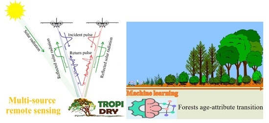
2.2.1. Multi-Source Remote-Sensing Data

Two types of data sets were used in this study: (1) a hyperspectral cube and (2) a large footprint full-waveform LiDAR data set. These two remote-sensing data sets were collected in March 2005 during the dry season. More specifically, the HyMapTM (HyVista Corporation Pty Ltd., Sydney, New South Wales, Australia) hyperspectral imagery, which is airborne remote-sensing data, was acquired on 4 March 2005, under cloud-free conditions [45,46]. This image data has 125 spectral bands ranging from 0.45 to 2.48 μm (15–20 nm of bandwidth intervals) and 15 m spatial resolution. Surface reflectance was derived from the original digital numbers using the HyCorr software (CSIRO, Canberra, Australia) following the steps described by Cao et al. (2015).
The large footprint full-waveform LiDAR data were collected using NASA’s Land, Vegetation and Ice Sensor (LVIS) system [45,46]. LVIS is an airborne, wide-swath imaging laser altimeter system that is flown over target areas to collect data on surface topography and 3-D structure. This system includes a 1064 nm-wavelength laser and three detectors. Additional information about the sensor can be found following the link of https://lvis.gsfc.nasa.gov/Home/index.html (accessed on 21 September 2021). The LiDAR data were collected within a week of the HyMap data. The LVIS system discretizes the return energy into 432 bins for each laser pulse emitted as a waveform that can represent the vertical distribution of the canopy well [47]. The nominal footprint size of these LiDAR data is 20 m. Gridded raster images were produced from the original binary point clouds stored in LVIS geo-located waveform (LGW) and LVIS ground elevation (LGE) data (version 1.02) for image fusion with hyperspectral data.

2.2.2. Forest Succession Reference Data Generation

A set of five remote-sensing images were used to generate the age data. The first images are a unique set of aerial photographs collected by the U.S. Army in 1956 (Scale 1:24,000), the second was a Landsat multispectral scanner image collected in January 1979 (60 m spatial resolution) eight years after the national park was created. The last images consist of three Landsat multispectral scanner images collected in January 1986, January 1997, and February 2005 (28.5 m spatial resolution) [15]. Those retrieved data were used to generate the forest age groups of 0–10, 10–20, 20–30, 30–50, and 50 + years used for age group mapping. Detailed steps for the generation of the reference data can be found in the work of [35], and this reference data enables the age group mapping. In this study, the age group variables (“AgeGroup”) were given parameters 1, 2, 3, 4, and 5 to represent the five age groups 0–10, 10–20, 20–30, 30–50, and 50 + years, respectively. The age group mapping result [35] is reproduced and used as a reference image presented in Figure 10a.

2.2.3. Ground Control Points

The same ground control points adopted by the authors of [35] were used in this study to validate mapping results. Ground control points were independently validated in July 2016 [15]. Specifically, 55 selected ground control points were obtained for each age group (1–5) based on the above-generated forest succession reference data, resulting in a total of 275 ground control points. These ground control points were then randomly divided into 30 training and 25 testing/validation samples per age group following [35].

3. Methods

3.1. Derivation of HyMap and LiDAR Metrics

Sun et al. [35] summarized and used twenty metrics from both HyMap and LiDAR data with the potential to map successional stages [10,33,34,48,49]. We used the same set of twenty metrics (9 LiDAR and 11 HyMap as summarized in Table 1) in this study. The HyMap metrics are biochemical and biophysical indices (CAI, LCA, NDNI, NDLI, DMCI, NDWI, SIWSI, NDTI, NDII, MSI, and RMSI) that were calculated using the SWIR wavelengths (1.2 to 1.38 μm, 1.4 to 1.79 μm, and from 1.91 to 2.48 μm) (see Sun et al., 2019 for a description on the indices). Those indices are relevant to the plant’s biochemical composition, structure, and water content. They are all different for different successional stages and therefore have been used for succession mapping. As described in the work of [35], CAI, LCA, NDNI, NDLI, and DMCI are five indices related to the lignin, cellulose, and nitrogen content of vegetation, whereas NDII, MSI, and RMSI are related to their water content [48,49]. NDWI, SIWSI, and NDTI are related to the biophysical structure of vegetation in a given successional stage. The LVIS metrics, namely Cx, Cy, RG, EC, MAX, RH50, AH1e10, AH1015, and AH1520, have demonstrated the potential to map TDFs succession [33,35]. Among them, Cx, Cy, and RG are three shape-based LiDAR metrics, whereas EC, MAX, and RH50 are point-based. The remaining three metrics are area-based.

3.2. Feature Selection from Multi-Source Fused Metrics

Only a small set of metrics can be of significance in differentiating successional stages [34]. As such, a feature selection approach was conducted in order to select only those metrics that are informative enough to explain data variance. In this study, a fast nonlinear feature learning model modified from a kernel archetypal analysis (KAA) [50,51] was developed to implement the feature selection. Moreover, Fourier features are demonstrated to be useful for efficient kernel learning [52,53]. Those studies indicate that the translation-invariant kernel function, such as K ( x 1 , x 2 ) , which is the inner product of feature vectors of ϕ ( x 1 ) and ϕ ( x 2 ) in the high dimensional kernel space, can also be expressed as the inner product of features vectors y ( x 1 ) and y ( x 2 ) in the low dimensional Euclidean space
K ( x 1 , x 2 ) = ϕ ( x 1 ) , ϕ ( x 2 ) = y ( x 1 ) T y ( x 2 )
This is because the translation-invariant kernel function can be regarded as the Fourier transform of a certain distribution p ( w ) in Equation (2)
K ( x 1 , x 2 ) = ϕ ( x 1 x 2 ) = R m p ( w ) e j w T ( x 1 x 2 ) d w
The Fourier transform can furthermore be approximately equivalent to the sum of the nonlinear functions generated by a finite number of expanded cosine basis functions:
R m p ( w ) e j w T ( x 1 x 2 ) d w i = 1 k 1 k e j w i T x 1 e j w i T x 2               = i = 1 k 1 k cos ( w i T x 1 + b i ) cos ( w i T x 2 + b i )               = 1 k y ( x 1 ) , 1 k y ( x 2 )
Therefore, the Fourier features were used in our study to approximate the Gaussian kernel K ( x , y ) = exp ( ( 1 / 2 σ 2 ) x y 2 ) in KAA to speed up the computation. Specifically, there are three essential steps for this approximation: (i) To randomly sample m parameters w i R M from the independent distribution p ( w ) as
w 1 , ,   w m ~ p ( w )
(ii) To construct a m -dimensional randomized feature map Y for the input data X as follows
y i = [ cos ( w i x 1 + b i ) , , cos ( w i x N + b i ) ] R N , Y = [ y 1 y m ] R m × N
Here, b i obeys the uniform distribution in the interval of w i ~ N ( 0 , 1 / σ 2 I ) . Finally, (iii) approximate the kernel matrix K with K ^
K K ^ = 1 m Y T Y
As the kernel was approximated with a randomized nonlinear feature map, we denote our feature extraction model as randomized nonlinear archetypal analysis (RNAA). RNAA was next used as the feature learning tool to generate G given number of features Z = { z 1 , z 2 , , z G } with both types of input metrics. The former was done by optimizing the objective function as follows:
min C , S | | X X C S | | F 2   s . t . C 0 ,   S 0 ,         | c g | 1 = 1 ,   | s k | 1 = 1
where X R N × K was input data with K features. The features, Z , are called archetypes, and they were generated as linear combinations of observations weighted by their index matrix C R K × G . The observations were reconstructed by these archetypes and the corresponding coefficient S R G × K .
In order to estimate which of the original input metrics are useful to explain the variance on the TDFs, and following the multiple endmember selection rules using the KAA model [51], the original input feature metrics, which contributed the most to the generation of each new transformed feature by RNAA were selected following Equation (8)
E g = { x i |   c g ( i ) > t h }
The acceptable threshold, th, is mean(max(cg) + min(cg)). Finally, the selected metrics used to generate the new features were integrated as the new input features of the age-attribute learning process.
Data from various data sources may have different expressions for a given object, and multi-source data fusion may obtain more abundant data information than what is necessary due to co-linearity and spatial autocorrelation. As such, independent learning from a single data source may be more beneficial to the discovery of important information than data integrated from two or more data sets. Because of this, feature selection using RNAA was first conducted on each individual remote-sensing data set to pick out the most informative metrics used for forest-age-attribute learning. The informative metrics selected from each data source were then fused in different combinations for forest-age-attribute learning. This was next compared with the learning performance of the independent source metrics to find out the most powerful fused metric set to map the forest succession of the study area.

3.3. Relative Attribute Learning for TDFs Succession Age Attribute

In this study, the relative attribute learning (RAL) algorithm integrated with the rank support vector machine (rankSVM) ranking model [38,39] was deployed to learn the relative relation of the age attribute (denoted as a function of the successional stage, as a ) of a given forest. Given the training data set X R N × G with G selected metric features, the RAL uses the relative relation between sample pairs and is treated as a “learn-to-rank” problem on the rankSVM framework (Equation (9) [38]).
min w w T 2 2 + C ( ε i j 2 + γ i j 2 ) s . t .   w T ( x i x j ) 1 ε i j , ( x i , x j ) O ,       | w T ( x i x j ) | γ i j ,   ( x i , x j ) S ,     ε i j 0 ,   γ i j 0
where ( x i , x j ) is a comparison pair of forest samples in X , w R G × 1 is the weight vector, C is the penalty factor, S and O are the similarity set and comparison set, respectively, which cannot be empty at the same time. The similarity set S requires the samples of each pair to have similar attributes, for example, forest samples with approximately the same age.
The ground control points used in this study have age group information (they have been assigned to the five age groups correspondingly) but no information on the specific forest age. As such, forest samples in the same age group may have different ages (For example, the early forests are among 0–10 years, but inside of the age group of 0–10, there are forests of 4, 7, and 9 years old). As it was not clear which pairs of the forest samples have the same age attribute, the similarity set S was set to empty to avoid uncertainty errors when learning the ranking function. The samples in different reference age groups were first used to construct a comparison set of the succession age attribute a to be used as part of a “learning ranking function”. Specifically, each point x i in the older age group was used to formulate the comparison pair O = { ( x i , x j ) | x i > a x j } with point x j in the younger age groups. The remaining twenty-five ground control points were also used this way in the accuracy assessment.
As part of the process associated with parameter setting, the penalty factor C for all the training data sets was not fixed as it was in Equation (9). Instead, our study assigned different penalty values to the training sample pairs since the more confident the training information is, the larger the penalty factor should be to make the model make fewer mistakes on the training data. As the similarity set was empty in our study, the specific value for the penalty was set as C S = 0 . Referring to the age group information, the forest samples in pairs that had a larger age gap were assumed to have more confident comparative relationships regarding their age attribute in the ranking function learning. If their ranking order (comparative relationship) was wrongly taken in training the ranking function, such comparative pairs were assigned a heavier penalty. On the contrary, if the forest samples had a smaller age gap, their age-attribute levels may be close to each other resulting in small intra-group/age variability. Under such circumstances, there is less confidence in imposing a heavy penalty to guarantee their ranking order in the learning. Therefore, for the pairs in the comparison set, the penalty was set as
C O i j = 200 * | AgeGroup i AgeGroup j |
This implies that the training sample pair with the larger age gap between two forest samples was given a larger C O i j . Thus, it was less likely for the model to make ranking errors on those training samples. With the prepared training data, the modified RankSVM model can be trained as follows:
min w w T 2 2 + C O i j ε i j 2 + C S γ i j 2 s . t .   w T ( x i x j ) 1 ε i j , ( x i , x j ) O ,       | w T ( x i x j ) | γ i j ,   ( x i , x j ) S ,     ε i j 0 ,   γ i j 0
Finally, the ranking score of a sample with respect to the succession age attribute can be obtained as seen in Equation (12):
r a = f ( x ) = w T x
Furthermore, r a was scaled to the range [0, 1] according to the maximum and minimum values of the relative scores R a of the whole forest following
r a = { r a min ( R a ) } / { max ( R a ) min ( R a ) }

3.4. Accuracy Assessment

In this study, the age attribute was evaluated via a ranking model. Therefore, the widely used Kendall’s τ was used to evaluate the quality of the ranking function [54], which was calculated via Equation (14)
τ = n con n incon N
where N is the total number of pairs, n con is the number of pairs in which the predicted relation between two samples is consistent with their true relation, and n incon is the number of pairs that have inconsistent estimated relation between two samples. Note, if x i = x j , r a i = r a j , the pair is neither counted as a consistent pair or an inconsistent pair. Specifically, if r a i > r a j for the pair { ( x i , x j ) | x i > A x j } , this pair is categorized as n con . Otherwise, it is categorized as n incon . The value will fall between −1 and 1. If τ = 1 , the sorting result is exactly the same as the benchmark sorting result. If τ = 0 , then there is no correlation between the two sets. If τ = 1 , the result of the ranking equation is completely opposite to that of the benchmark.

4. Results

4.1. HyMap and LVIS Metrics Selection and Age-Attribute Learning

Different configurations of metrics were conducted for age-attribute learning and performance evaluation. Specifically, the number G in the developed method of RNAA varied from 1 to the number of input metrics used to implement feature learning. Then a different configuration of metrics that contribute to the generation of a new feature was indirectly achieved following Equation (8) with the optimized index matrix C . These steps were first conducted on the remote-sensing data set from the independent source. On each data set, the varied configuration of metrics was compared to analyze their different potential for age-attribute learning. After that, the most informative configuration of metrics of both data sets was combined together, and the same feature selection process was conducted on the combined data to analyze the most informative fused metrics.

4.1.1. Metric Selection of HyMap Data of SRNP-EMSS

Table 2 lists the key metric selection results from HyMap data collected at SRNP-EMSS, conducted following the rules of Equation (8). Using a different number of RNAA features to explain the data variance at SRNP-EMSS enabled the discovery of a different number of informative metrics. As can be seen in Table 2 and Figure 2, the ranking accuracies achieved on training and test data sets fluctuate when less than four metrics are used. Even though the training and test accuracies see a nearly sustained growth when more than four metrics are being used, and contrary to the training accuracy, the test accuracy begins to decrease after more than nine metrics are being used (shown in Figure 2). Both accuracies increased after the introduction of the NDNI, NDLI, DMCI, and MSI metrics. Of these metrics, NDNI, NDLI, and DMCI use the SWIR wavelengths, and MSI uses the VNIR wavelengths.
Along with those quantitative results, Figure 3 further presents the qualitative age-attribute mapping results for the whole study area. Visual comparisons with the reference age data of our study area suggest that the feature learning results RNAA(4), RNAA(5), and RNAA(7) are all feasible. Concerning goodness of fit, the most informative set of HyMap metrics extracted by RNAA to evaluate the forest age groups of the study area are considered to be NDNI, NDLI, DMCI and MSI learned via RNAA(4) (Table 2 and Figure 2).
As can be seen in Figure 4, NDNI, NDLI, and DMCI are in diagonally opposed quadrants, and as such, they are the most dominant feature variables to explain data variance. As this result agrees with the feature selection results, we conclude that NDNI, NDLI, DMCI, and MSI are the most important metrics for the HyMap data.

4.1.2. Metric Selection of LVIS Data of SRNP-EMSS

A similar learning process to the one described above in the context of the HyMap metrics was conducted with the LVIS metrics. As can be observed in Table 3 and Figure 5, both training and test accuracies increase immediately when using the metric set Cx, RG, MAX, EC, and RH50 (selected by the RNAA (2)), and after this, the accuracies fluctuate slightly upon the introduction of additional metrics. However, the test accuracies stay below the highest accuracy achieved using the RNAA (2), even when more metrics are added (Table 3 and Figure 5).
The age-attribute learning results, shown in Table 3 and Figure 5, are represented in a spatial context in Figure 6. This figure suggests that the combination of Cx, RG, MAX, EC, and RH50, selected by RNAA(2), is the most powerful set of metrics that avoids the under- and over-fitting problem.
The LVIS metric variables in the space of the first two principal components are presented in Figure 7. As suggested by this figure, the metric set of RG, MAX, EC, and RH50 are more dominant loading factors than the other metrics. More importantly, RH50 approaches orthogonality to RG, MAX, EC, Cx, and AH1015. In particular, RH50, Cx, MAX, and AH1015 are distributed in four different quadrants. Therefore, a combination of these metrics would achieve maximum information complementarity. These dominant metrics are overlapped with the key metric set of Cx, RG, MAX, EC, and RH50, which performed the best in age-attribute learning.

4.1.3. Multi-Source Metric Fusion

Table 4 illustrates the key metrics from HyMap and LVIS data for TDF age learning at SRNP-EMSS under different metric fusion conditions. Here, training data has a higher age-attribute learning accuracy ( τ = 0.9418 ) than the highest accuracy achieved on the independent data set (either HyMap or LVIS). However, the test accuracy ( τ = 0.8806 ) is lower than the highest accuracies obtained on the two independent data sets. To test the ability to improve the result, a smaller fusion data set was compiled by fixing the key metrics from one data source and adding one key metric from the other data source. In the case of using the HyMap key metrics with one informative LiDAR key metric, nearly all training and test accuracies increased when compared to the best cases achieved on the independent data. The only combination of a decreased accuracy was that of the NDNI, NDLI, DMCI, MSI, and MAX metric set. In this case, the test accuracy was slightly lower than that obtained without adding MAX. Here, RH50 was found to be the best LiDAR metric to be combined with the hyperspectral metric set.
The results, shown in Table 4, can be summarized as follows: Adding one hyperspectral metric to a set of dominant LVIS metrics achieved a better performance than using the dominant hyperspectral metrics with one added LVIS metric. In previous sections, the LiDAR metrics were also found to be more powerful than the hyperspectral metrics for the evaluation of the TDF’s successional age attribute at SRNP-EMSS. The metric set included NDNI, Cx, RG, MAX, EC, and RH50, which enabled the analysis of fused data to provide the best performance, are displayed in Figure 8 in the space of the first two principal components. As can be seen in that figure, the metric NDNI is orthogonal to all the rest of the LiDAR metrics and thus provides suitable complementarity for the other metrics.
Table 5 illustrates the differences before and after the best LiDAR metrics were fused with the NDNI metric. As can be seen in the table, the importance/weight of the LVIS metrics changed with the introduction of the NDNI variable, which led to an improvement in the ranking accuracy.

4.2. Age-Attribute Mapping

The ranking scores of the age attribute, achieved using the metric set NDNI, Cx, RG, MAX, EC, and RH50 on 125 test samples, are presented in Figure 9. With the ascending age groups, each of which has 25 forest samples, an overall increasing trend in the relative scores of the age attribute can be observed. Moreover, the 25 forest samples within each age group were predicted using different levels of the age attribute.
Figure 10b shows the age-attribute mapping results for the whole study area, whereas the age group mapping result of the previous study by the authors of [35] is reproduced and presented in Figure 10a for comparison. Compared to discrete age group mapping, the relative scores of the age-attribute mapping offer a continuous transition of the succession process as well as a quantitative evaluation for the composition of the age variations in each discrete age group. These variations can be seen more intuitively in the filled contour map of the relative scores of the age-attribute mapping, shown in Figure 10c. As can be seen in that figure, one discrete age group contains areas that are of different ages. The statistical histogram of the relative scores of the age-attribute mapping result, shown in Figure 10d, suggests that the number of pixels increases from young forests toward mature forests until the relative score of the age attribute becomes 0.8. Thus, there are fewer pixels in the young and old forest categories than in the categories in between.

4.3. Statistical Analysis

Figure 11 shows the statistics related to the spatial and statistical distribution of pixels in different age groups. As can be seen in the upper row of the figure, the number of pixels in the old category (shown in red) increases from the early forest category to the mature forest category. As seen in the maps of the middle row, the number of pixels that fall under different age scores (a) increases as a function of increasing age until the most mature age group and (b) overlaps between the neighboring age groups.
The probability density function (PDF) curves, fitted from the above-derived histogram and shown in Figure 12, suggest clear succession transitions of the five age groups. Transition patterns from one age group to another can be visually observed from the statistic mean of the PDF curve, corresponding to each predefined age group. Except for the age groups of 0–10 years and 50+ years, forests in all the other periods were predicted with the age-attribute level across a score range width approaching 0.5. For example, for the 10–20 years period, the age-attribute relative score varied approximately from 0.2 to 0.7, for the 20–30 year period from 0.4 to 0.9, and for the 30–50 year period, from 0.5 to 1.0. However, a very different phenomenon was observed for the early and late age groups. For the early period, the age-attribute level was estimated with a range of 0 to 0.6, and for the late/mature age, the range was 0.7 to 1.0. Thus, the age-attribute-level range is either wider (young age) or narrower (mature age) than the age-attribute-level range of the intermediate periods. Most pixels fell into the intermediate age range.
Boxplots in Figure 13 show an overall ascending trend of the medians, minima, and maxima of the age scores as a function of the increasing age group. Specifically, the average relative level of the age attribute for each age group was predicted as 0.3296, 0.4313, 0.6148, 0.7333, and 0.8180 for the five age groups, correspondingly. If year zero was taken as the minimum and year 60 was taken as the maximum, the above-average levels/scores would represent years 19, 25, 36, 43, and 48, correspondingly. As shown in Figure 13, the standard deviation is relatively high (σ = 0.1104) for the youngest age group and relatively low (σ = 0.06) for the most mature age group. Those age groups in between vary from σ = 0.0827 (30–50 years) to σ = 0.0893 (10–20 years) and σ = 0.0933 (20–30 years). This implicitly points to some intra-group age variability of the age groups of the study area.

5. Discussion

For the past few decades, studies on the regeneration of TDFs have extensively characterized the process as three deterministic successional stages, i.e., early, intermediate, and late. Li et al. [34] tried to treat the regrowth process of secondary TDFs as a continuous process by evaluating the intermediate successional stage with three sub-classes of early-intermediate, intermediate-intermediate, and intermediate-late, which provides a more detailed transition between adjacent growth stages. In this study, we evaluated the TDF succession at SRNP-EMSS using the age attribute instead of successional stages or age groups. The development of pathways and ecosystem dynamics of the SRNP-EMSS study area was quantified at detailed relative levels of the age attribute without knowing the exact growth age of any particular area. Here, we discuss the implications of our results with respect to the metric selection, ecological importance, and successional transitions.

5.1. Significance of Key Metric Selection

Different features are of different levels of importance to the identification task. Simple concatenation or stacking of different features for the research object may contain redundant information or lead to over-fitting when limited training samples are available. Thus, it is essential to conduct feature reduction when using multi-dimensional hyperspectral and full-waveform LiDAR metric data [55]. To this end, correlation matrix computation [34] and multiple comparison analyses [33,35] were used. Feature transformation is one of the main strategies of feature reduction as it has the ability to use more complex linear or nonlinear mathematics to generate some explainable features for the data variance. However, in ecological studies, it is highly important to pick out the most informative features from the original set rather than using virtual mathematic features to reveal the functional relationship between these features and the physical or chemical traits of the object. In this study, a fast nonlinear feature selection tool-RNAA was used to derive the key hyperspectral and LiDAR metrics. RNAA was implemented to select the most informative spectral indices and LiDAR metrics. This process tracked the contribution of the original input metrics to mathematic features in the feature transformation so that informative metrics were extracted following rules in Equation (5). Similar processing strategies have been adopted in endmember extraction studies [51,56] via archetypal analysis, which has a suitable model interpretation ability and has demonstrated the ability to work when multiple representative sample selections need to be conducted.
Results summarized in Table 2 and Table 3 show that using more metrics in learning did not necessarily result in a more precise predicting accuracy. Such a conclusion was also derived when using LiDAR and hyperspectral data for aboveground biomass modeling in the Brazilian Amazon [55]. Figure 4 and Figure 7 show some feature redundancy in the PCA feature space. Even though the training accuracy could be seen growing with a larger metric set, the test accuracy decreased once the used metrics reached a certain number, suggesting over-fitting. As shown in Table 4, the fusion of key metrics, generated from hyperspectral and full-waveform LiDAR data, have the potential for TDF succession learning in the SRNP-EMSS study area. This has also been documented in former studies [34,35]. It needs to be highlighted that our study used only five metrics, namely NDNI, Cx, RG, MAX, EC, and RH50, which have been found to be the optimal set to improve succession learning. Evaluating different metric combinations in the context of feature redundancy and potential over-fitting guaranteed achieving the optimal mapping results shown in Table 4.

5.2. Ecological Importance of the Key Metrics Used for Age-Attribute Learning

Secondary TDFs include changing horizontal (e.g., canopy openness and homogeneity) and vertical (e.g., canopy height, LAI) structures and species compositions driven by wind-dispersed or vertebrate-dispersed mechanisms [15,57,58]. To effectively evaluate the succession processes, these horizontal and vertical variables that are relevant to forest growth and their biochemical and biophysical expressions need to be considered.
The biochemical expressions of the forests can be analyzed using spectral data. In our study, NDNI, NDLI, DMCI, and MSI were found to be the most potent metrics to be used for age-attribute learning. Of these metrics, NDNI, in particular, demonstrated its power in discriminating the age-attribute level of the succession process, as it enabled the best age-attribute learning results to be obtained when fused with the LiDAR metrics (Table 4). Among the spectral indices, NDNI is used to estimate the relative content of nitrogen in vegetation canopy and has been demonstrated to be very sensitive to the change of nitrogen content when the vegetation is still green [59]. Nitrogen is an important component of chlorophyll, and vegetation with a high concentration of nitrogen grows faster. A study of [17] indicated that early successional communities may be more nitrogen-limited [60] than later successional stages due to reduced rates of decomposition associated with high C:N ratios. In contrast, intermediate and older communities were dominated by fast-growing species with higher C:N ratios, higher growth rates, and forest net primary productivity [61]. Both leaf C:N ratio and leaf dry matter concentration (factors that relate to NDNI and DMCI metrics, respectively) were found to be relatively low during the earlier stages of succession and were maximized during the intermediate stages of succession [17]. These findings can partially explain the performance of the NDNI in the evaluation of the forest growth status related to the age attribute. Gei et al. [62] have indicated that a higher density of nitrogen-fixing species exists in the early stages. In fact, it is has been found that most of the recovery of species richness and species composition occurs in younger secondary forests [63].
The hyperspectral remote-sensing data of this study were collected during the dry season. In the dry season, there are nearly no leaves in the early successional forests, which are mixtures of woody vegetation, shrubs, and pastures. In the intermediate successional forests, up to 80% are deciduous with fast-growing trees and lianas, whereas in the late successional forests, 50–90% of the canopy is occupied by evergreen crowns with three layers of vegetation [23,26]. In the absence of leaves, the spectral separability of a forest is largely driven by carbon constituents, such as bark and litter-fall, detectable using the SWIR wavelength region [10,64]. Moreover, older forests with more biomass and higher water content are found to have higher absorption and, thereby, lower reflectance in the SWIR [65]. Because of these physico-chemical factors, spectral indices such as NDNI, NDLI, DMCI, and MSI, associated with the relative wood content, nutrients, and water content of the canopy, can be successful in the detection of the successional stages.
Growth patterns can be mainly detected by analyzing the vertical structures of a forest [66]. In this context, full-waveform LiDAR data has shown its potential for studying TDF succession (e.g., [15,33]). Evidence shows that the elevation of the major peak and the maximum amplitude of the waveform present a regular trend for the successional stages, the former increasing and the latter decreasing from the early to the late stage (e.g., the work of [33]). Their study used line-, point-, shape- and area-based groups of metrics to differentiate the successional stages. Their results further indicate that all nine LiDAR metrics used in the study (Cx, Cy, and RG are shape-based, EC, MAX, and RH50 are point-based and AHle 10 , AHle1015, and AH 1520 are the area-based metrics) were significantly different at the three successional stages of the SRNP-EMSS. They furthermore demonstrated that even if the late and intermediate successional stages could be identified by any of the four metric groups, the intermediate successional stage could not be identified exclusively based on the line-based metrics, and the early successional stage could be identified neither by the point- nor by the area-based metrics. Three point-based LiDAR waveform metrics, i.e., RH 25 , RH 50 , and RH 100 were also used by the authors of [27] to characterize successional stages in SRNP-EMSS. In our study, a combination of shape- and point-based groups of metrics, namely, Cx, RG , MA X , EC and RH 50 , were found to be the smallest subset of the LiDAR metrics to fully explain the successional variation in the study area.

5.3. TDFs Succession Transition with Respect to Age Attribute

Secondary TDFs are compositional mosaics driven by ecological and biophysical processes. For instance, the study by Waring et al. [67], also conducted in Santa Rosa, Costa Rica, highlights the high variability in stand ages, soil properties, and orthogonal gradients of the successional stages. In our study, the varying levels of the age attribute shown in Figure 10b provided visual evidence that the TDF succession process in the study area was learned as continuous transition trajectories. These trajectories are expressed with dynamic relative levels of the forest age attribute rather than deterministic ecological processes [34]. Evaluation of the relative strength of the age attribute to characterize the ecological transitions in a secondary TDF is more objective than the identification of the secondary TDF succession transitions with absolute age or rough stages that do not take the intra-class variability into account. Because the forest attributes in the remote-sensing images are in general mixed at the pixel level, they are related to a combination of ecological and biophysical variables [10,22]. As seen in Figure 11, our study encountered detailed age variation within the five age groups. The overlapping age-attribute levels, shown in Figure 12, visualize the transition patterns of the age variations between the different succession stages.
In this study, forests in the early succession stage had the highest standard deviations of the age attribute (Figure 13). This conforms to the finding by Gu et al. [33], who encountered large differences in the vertical structures of the early successional stages revealed by the standard deviations of the LiDAR waveforms. Gu et al. [33] also mentioned that the forest structures in the intermediate and late successional stages were more uniform, and the standard deviations for these two successional stages were similar at all LiDAR waveform elevation levels. In our study, forests in the age group of 50+ years were found to have the smallest standard deviation of the age-attribute level when compared with the younger age groups. It is reasonable to assume that this is due to the uniformity of the vertical structures of the most mature successional stage. Moreover, the standard deviations of the three intermediate age groups were similar to one another, and the values were in between the youngest and oldest age groups. Overall, the standard deviations of the age attribute decreased from the early period toward the late/mature period.

6. Conclusions

This paper investigated the potential of multi-source, full-waveform LiDAR and hyperspectral remote-sensing data fusion for the evaluation of the forest age in the SRNP-EMSS study area. A total of 20 metrics, 11 derived from full-waveform LiDAR data and 9 derived from hyperspectral data, were used to mine for the smallest number of informative metrics with a potential for age-attribute learning. This was achieved through a fast feature selection tool of an RNAA model and the RAL model. The RNAA model was used to nonlinearly transform the original input metric features into newly generated metrics, and the RAL model was deployed to provide relative age levels of the TDFs in the study area. The most important findings of this process can be summarized as follows:
(1)
Of the hyperspectral metrics used in this study, NDNI, NDLI, DMCI, and MSI selected by the RNAA model were found to be the best set of variables to explain the data variance and, ultimately, the forest age variation of the study area;
(2)
A combination of the shape-based (Cx, RG) and point-based (MAX, EC and RH50) LiDAR metrics, selected by the RNAA model and extracted from the LVIS data, were found to be the smallest number of the LiDAR metrics that best explained the forest age variation of the study area;
(3)
Fusing hyperspectral and LiDAR data achieved better results than using these data sets independently. Of the parameters used in this study, NDNI, Cx, RG, MAX, EC, and RH50 were found to be the most powerful combination to map the forest age variation of the study area;
(4)
The RAL method was successfully used to retrieve the relative age-attribute degree of TDFs in the study area. The result is a continuous forest age-level map that covers the successional stages of the study area;
(5)
A comparison between the former age group mapping result by Sun et al. (2019) and ours confirms that the TDF succession process in the study area can be well understood as continuous transition trajectories expressed with dynamic relative levels of the forest age attribute, rather than deterministic ecological processes. Descending standard deviations of the age attribute were observed along the transition trajectories, which account for the varied uniformity of the vertical structures along the process of forest succession.

Author Contributions

G.Z. made contributions on conceptualization, methodology development, original draft preparation, review and editing and funding support. A.S.-A. contributed on data resources providing, supervision, review and editing, as well as funding support. K.L. provided great effort on review and editing. C.S. helped with resources providing. L.F. provided advice and funding support. All authors have read and agreed to the published version of the manuscript.

Funding

This work was funded by the Inter-American Institute for Global Change 770 Research (IAI) Collaborative Research Network program (CRN2-021 and CRN3-025)—U.S. National Science Foundation (Grant GEO 0452325); the National Science and Engineering Research Council of Canada (NSERC-Discovery); and the National Natural Science Foundation of China (No. 61701123). It is also partially funded by National High-Resolution Earth Observation Major Project (83-Y40G33-9001-18/20) and the Natural Science Foundation of Guangdong Province (2019A1515011811). We also thank the support from the China Scholar Council (CSC).

Conflicts of Interest

The authors declare no conflict of interest.

References

  1. Myers, N. The world’s forests: Problems and potentials. Environ. Conserv. 1996, 23, 156–168. [Google Scholar] [CrossRef]
  2. Ingram, J.C.; Dawson, T.; Whittaker, R. Mapping tropical forest structure in southeastern Madagascar using remote sensing and artificial neural networks. Remote Sens. Environ. 2005, 94, 491–507. [Google Scholar] [CrossRef]
  3. Olson, D.M.; Dinerstein, E.; Wikramanayake, E.D.; Burgess, N.D.; Powell, G.V.N.; Underwood, E.C.; D’Amico, J.A.; Itoua, I.; Strand, H.E.; Morrison, J.C.; et al. Terrestrial ecoregions of the world: A new map of life on earth: A new global map of terrestrial ecoregions provides an innovative tool for conserving biodiversity. Bioscience 2001, 51, 933–938. [Google Scholar] [CrossRef]
  4. Janzen, D.H. Tropical Ecological and Biocultural Restoration. Science 1988, 239, 243–244. [Google Scholar] [CrossRef] [PubMed]
  5. Hoekstra, J.M.; Boucher, T.M.; Ricketts, T.H.; Roberts, C. Confronting a biome crisis: Global disparities of habitat loss and protection. Ecol. Lett. 2004, 8, 23–29. [Google Scholar] [CrossRef]
  6. Portillo-Quintero, C.; Sánchez-Azofeifa, G. Extent and conservation of tropical dry forests in the Americas. Biol. Conserv. 2010, 143, 144–155. [Google Scholar] [CrossRef]
  7. Portillo-Quintero, C.; Sanchez-Azofeifa, A.; Calvo-Alvarado, J.C.; Quesada, M.; Santo, M.M.D.E. The role of tropical dry forests for biodiversity, carbon and water conservation in the neotropics: Lessons learned and opportunities for its sustainable management. Reg. Environ. Chang. 2014, 15, 1039–1049. [Google Scholar] [CrossRef]
  8. Calvo-Rodriguez, S.; Sanchez-Azofeifa, A.G.; Duran, S.M.; Espírito-Santo, M.M. Assessing ecosystem services in Neotropical dry forests: A systematic review. Environ. Conserv. 2016, 44, 34–43. [Google Scholar] [CrossRef]
  9. How to grow a tropical national park: Basic philosophy for Guanacaste National Park, northwestern Costa Rica. Experientia 1987, 43, 1037–1038. [CrossRef]
  10. Cao, S.; Yu, Q.; Sanchez-Azofeifa, A.; Feng, J.; Rivard, B.; Gu, Z. Mapping tropical dry forest succession using multiple criteria spectral mixture analysis. ISPRS J. Photogramm. Remote Sens. 2015, 109, 17–29. [Google Scholar] [CrossRef]
  11. Chazdon, R.L.; Broadbent, E.N.; Rozendaal, D.M.A.; Bongers, F.; Zambrano, A.M.A.; Aide, T.M.; Balvanera, P.; Becknell, J.M.; Boukili, V.; Brancalion, P.H.S.; et al. Carbon sequestration potential of second-growth forest regeneration in the Latin American tropics. Sci. Adv. 2016, 2, e1501639. [Google Scholar] [CrossRef] [PubMed] [Green Version]
  12. Oliveira, R.A.; Tommaselli, A.M.; Honkavaara, E. Generating a hyperspectral digital surface model using a hyperspectral 2D frame camera. ISPRS J. Photogramm. Remote Sens. 2018, 147, 345–360. [Google Scholar] [CrossRef]
  13. Sanchez-Azofeifa, G.A.; Kalacska, M.; Quesada, M.; Calvo-Alvarado, J.C.; Nassar, J.M.; Rodriguez, J.P. Need for integrated research for a sustainable future in tropical dry forests. Conserv. Biol. 2005, 19, 285–286. [Google Scholar] [CrossRef]
  14. Sánchez-Azofeifa, G.A.; Pfaff, A.; Robalino, J.A.; Boomhower, J.P. Costa Rica’s payment for environmental services program: Intention, implementation, and impact. Conserv. Biol. 2007, 21, 1165–1173. [Google Scholar] [CrossRef] [Green Version]
  15. Sánchez-Azofeifa, G.A.; Guzmán-Quesada, J.A.; Vega-Araya, M.; Campos-Vargas, C.; Durán, S.M.; D’Souza, N.; Gianoli, T.; Portillo-Quintero, C.; Sharp, I. Can terrestrial laser scanners (TLSs) and hemispherical photographs predict tropical dry forest succession with liana abundance? Biogeosciences 2017, 14, 977–988. [Google Scholar] [CrossRef] [Green Version]
  16. Quesada, M.; Sanchez-Azofeifa, A.; Alvarez-Añorve, M.; Stoner, K.E.; Avila-Cabadilla, L.; Calvo-Alvarado, J.C.; Castillo, A.; Espírito-Santo, M.M.; Fagundes, M.; Fernandes, G.W.; et al. Succession and management of tropical dry forests in the Americas: Review and new perspectives. For. Ecol. Manag. 2009, 258, 1014–1024. [Google Scholar] [CrossRef]
  17. Buzzard, V.; Hulshof, C.M.; Birt, T.; Violle, C.; Enquist, B.J. Re-growing a tropical dry forest: Functional plant trait composition and community assembly during succession. Funct. Ecol. 2015, 30, 1006–1013. [Google Scholar] [CrossRef] [Green Version]
  18. Castro, K.L.; Sanchez-Azofeifa, G.A.; Rivard, B.; Sanchez-Azofeifa, A. Monitoring secondary tropical forests using space-borne data: Implications for Central America. Int. J. Remote Sens. 2003, 24, 1853–1894. [Google Scholar] [CrossRef]
  19. Prach, K.; Walker, L.R. Four opportunities for studies of ecological succession. Trends Ecol. Evol. 2011, 26, 119–123. [Google Scholar] [CrossRef]
  20. Becknell, J.M.; Powers, J.S. Stand age and soils as drivers of plant functional traits and aboveground biomass in secondary tropical dry forest. Can. J. For. Res. 2014, 44, 604–613. [Google Scholar] [CrossRef]
  21. Arroyo-Mora, J.P.; Sanchez-Azofeifa, G.A.; Kalacska, M.; Rivard, B.; Calvo-Alvarado, J.C.; Janzen, D.H. Secondary forest detection in a neotropical dry forest landscape using Landsat 7 ETM+ and IKONOS imagery1. Biotropica 2005, 37, 497–507. [Google Scholar] [CrossRef]
  22. Kalacska, M.E.R.; Sánchez-Azofeifa, G.A.; Calvo-Alvarado, J.C.; Rivard, B.; Quesada, M. Effects of season and successional stage on leaf area index and spectral vegetation indices in three Mesoamerican tropical dry forests. Biotropica 2005, 37, 486–496. [Google Scholar] [CrossRef]
  23. Kalacska, M.; Sanchez-Azofeifa, A.; Calvo-Alvarado, J.C.; Quesada, M.; Rivard, B.; Janzen, D. Species composition, similarity and diversity in three successional stages of a seasonally dry tropical forest. For. Ecol. Manag. 2004, 200, 227–247. [Google Scholar] [CrossRef]
  24. Kalacska, M.; Sanchez-Azofeifa, G.A. Hyperspectral Remote Sensing of Tropical and Sub-Tropical Forests; Kalacska, M., Sanchez-Azofeifa, G.A., Eds.; CRC Press: Boca Raton, FL, USA, 2008; ISBN 9780429136702. [Google Scholar]
  25. Kalacska, M.; Sanchez-Azofeifa, G.; Rivard, B.; Caelli, T.; White, H.P.; Calvo-Alvarado, J.C. Ecological fingerprinting of ecosystem succession: Estimating secondary tropical dry forest structure and diversity using imaging spectroscopy. Remote Sens. Environ. 2007, 108, 82–96. [Google Scholar] [CrossRef]
  26. Castillo-Núñez, M.; Sánchez-Azofeifa, G.A.; Croitoru, A.; Rivard, B.; Calvo-Alvarado, J.C.; Dubayah, R.O. Delineation of secondary succession mechanisms for tropical dry forests using LiDAR. Remote Sens. Environ. 2011, 115, 2217–2231. [Google Scholar] [CrossRef]
  27. Castillo, M.; Rivard, B.; Sanchez-Azofeifa, A.; Calvo-Alvarado, J.C.; Dubayah, R. LIDAR remote sensing for secondary Tropical Dry Forest identification. Remote Sens. Environ. 2012, 121, 132–143. [Google Scholar] [CrossRef]
  28. Martinuzzi, S.; Gould, W.; Vierling, L.A.; Hudak, A.T.; Nelson, R.F.; Evans, J. Quantifying tropical dry forest type and succession: Substantial improvement with LiDAR. Biotropica 2012, 45, 135–146. [Google Scholar] [CrossRef] [Green Version]
  29. Abshire, J.B.; Sun, X.; Riris, H.; Sirota, J.M.; McGarry, J.F.; Palm, S.; Yi, D.; Liiva, P. Geoscience Laser Altimeter System (GLAS) on the ICESat Mission: On-orbit measurement performance. Geophys. Res. Lett. 2005, 32, L21S02. [Google Scholar] [CrossRef] [Green Version]
  30. Lindberg, E.; Olofsson, K.; Holmgren, J.; Olsson, H. Estimation of 3D vegetation structure from waveform and discrete return airborne laser scanning data. Remote Sens. Environ. 2012, 118, 151–161. [Google Scholar] [CrossRef] [Green Version]
  31. Armston, J.; Disney, M.; Lewis, P.; Scarth, P.; Phinn, S.; Lucas, R.; Bunting, P.; Goodwin, N. Direct retrieval of canopy gap probability using airborne waveform lidar. Remote Sens. Environ. 2013, 134, 24–38. [Google Scholar] [CrossRef]
  32. Milenković, M.; Schnell, S.; Holmgren, J.; Ressl, C.; Lindberg, E.; Hollaus, M.; Pfeifer, N.; Olsson, H. Influence of footprint size and geolocation error on the precision of forest biomass estimates from space-borne waveform LiDAR. Remote Sens. Environ. 2017, 200, 74–88. [Google Scholar] [CrossRef]
  33. Gu, Z.; Cao, S.; Sanchez-Azofeifa, G. Using LiDAR waveform metrics to describe and identify successional stages of tropical dry forests. Int. J. Appl. Earth Obs. Geoinf. 2018, 73, 482–492. [Google Scholar] [CrossRef]
  34. Li, W.; Cao, S.; Campos-Vargas, C.; Sanchez-Azofeifa, A. Identifying tropical dry forests extent and succession via the use of machine learning techniques. Int. J. Appl. Earth Obs. Geoinf. 2017, 63, 196–205. [Google Scholar] [CrossRef]
  35. Sun, C.; Cao, S.; Sanchez-Azofeifa, G.A. Mapping tropical dry forest age using airborne waveform LiDAR and hyperspectral metrics. Int. J. Appl. Earth Obs. Geoinf. 2019, 83, 101908. [Google Scholar] [CrossRef]
  36. Lucas, R.; Honzák, M.; Curran, P.J.; Foody, G.; Milne, R.; Brown, T.; Amaral, S. Mapping the regional extent of tropical forest regeneration stages in the Brazilian Legal Amazon using NOAA AVHRR data. Int. J. Remote Sens. 2000, 21, 2855–2881. [Google Scholar] [CrossRef]
  37. Kalacska, M.; Calvo-Alvarado, J.C.; Sanchez-Azofeifa, G.A. Calibration and assessment of seasonal changes in leaf area index of a tropical dry forest in different stages of succession. Tree Physiol. 2005, 25, 733–744. [Google Scholar] [CrossRef] [PubMed] [Green Version]
  38. Parikh, D.; Grauman, K. Relative attributes. In Proceedings of the IEEE International Conference on Computer Vision, Barcelona, Spain, 6–13 November 2011; pp. 503–510. [Google Scholar]
  39. Zhao, G.; Cheng, L.; Wu, H.; Li, H.; Li, X. Relative attribute based unmixing. In Proceedings of the IEEE International Geoscience and Remote Sensing Symposium, Valencia, Spain, 22–27 July 2018; pp. 2705–2708. [Google Scholar]
  40. Cao, S.; Sanchez-Azofeifa, A. Modeling seasonal surface temperature variations in secondary tropical dry forests. Int. J. Appl. Earth Obs. Geoinf. 2017, 62, 122–134. [Google Scholar] [CrossRef]
  41. Sánchez-Azofeifa, G.A.; Quesada, M.; Rodríguez, J.P.; Nassar, J.M.; Stoner, K.E.; Castillo, A.; Garvin, T.; Zent, E.L.; Calvo-Alvarado, J.C.; Kalacska, M.E.; et al. Research priorities for neotropical dry forests. Biotropica 2005, 37, 477–485. [Google Scholar] [CrossRef]
  42. Calvo-Rodriguez, S.; Sánchez-Azofeifa, G.A.; Durán, S.M.; Espírito-Santo, M.M.D.; Nunes, Y.R.F. Dynamics of carbon accumulation in tropical dry forests under climate change extremes. Forests 2021, 12, 106. [Google Scholar] [CrossRef]
  43. Kalacska, M. Leaf area index measurements in a tropical moist forest: A case study from Costa Rica. Remote Sens. Environ. 2004, 91, 134–152. [Google Scholar] [CrossRef]
  44. Quesada, M.; Stoner, K.E. Threats to the conservation of tropical dry forest in Costa Rica. In Biodiversity Conservation in Costa Rica Learning the Lessons in a Seasonal Dry Forest; University of California Press: Los Angeles, CA, USA, 2004; pp. 266–280. ISBN 0520223098. [Google Scholar]
  45. Blair, J.; Rabine, D.L.; Hofton, M.A. The laser vegetation imaging sensor: A medium-altitude, digitisation-only, airborne laser altimeter for mapping vegetation and topography. ISPRS J. Photogramm. Remote Sens. 1999, 54, 115–122. [Google Scholar] [CrossRef]
  46. Hofton, M.; Rocchio, L.; Blair, J.; Dubayah, R. Validation of vegetation canopy lidar sub-canopy topography measurements for a dense tropical forest. J. Geodyn. 2002, 34, 491–502. [Google Scholar] [CrossRef]
  47. Fukushima, Y.; Hiura, T.; Tanabe, S.-I. Accuracy of the MacArthur-Horn method for estimating a foliage profile. Agric. For. Meteorol. 1998, 92, 203–210. [Google Scholar] [CrossRef]
  48. Casas, A.; Riano, D.; Ustin, S.; Dennison, P.; Salas, J. Estimation of water-related biochemical and biophysical vegetation properties using multitemporal airborne hyperspectral data and its comparison to MODIS spectral response. Remote Sens. Environ. 2014, 148, 28–41. [Google Scholar] [CrossRef]
  49. Ferreira, M.P.; Zortea, M.; Zanotta, D.C.; Shimabukuro, Y.E.; Filho, C.R.D.S. Mapping tree species in tropical seasonal semi-deciduous forests with hyperspectral and multispectral data. Remote Sens. Environ. 2016, 179, 66–78. [Google Scholar] [CrossRef]
  50. Mørup, M.; Hansen, L.K. Archetypal analysis for machine learning and data mining. Neurocomputing 2012, 80, 54–63. [Google Scholar] [CrossRef]
  51. Zhao, C.; Zhao, G.; Jia, X. Hyperspectral image unmixing based on fast kernel archetypal analysis. IEEE J. Sel. Top. Appl. Earth Obs. Remote Sens. 2016, 10, 331–346. [Google Scholar] [CrossRef]
  52. Yang, T.; Li, Y.F.; Mahdavi, M.; Jin, R.; Zhou, Z.H. Nyström method vs. random Fourier features: A theoretical and empirical comparison. In Proceedings of the Advances in Neural Information Processing Systems, Lake Tahoe, NV, USA, 3–8 December 2012; pp. 476–484. [Google Scholar]
  53. Rahimi, A.; Recht, B. Random features for large-scale kernel machines. In Proceedings of the International Conference on Advances in Neural Information Processing Systems, Whistler, BC, Canada, 6–10 December 2009; pp. 1177–1184. [Google Scholar]
  54. Liang, L.; Grauman, K. Beyond comparing image pairs: Setwise active learning for relative attributes. In Proceedings of the IEEE International Conference on Computer Vision and Pattern Recognition, Columbus, OH, USA, 23–28 June 2014; pp. 208–215. [Google Scholar]
  55. de Almeida, C.T.; Galvão, L.S.; Aragão, L.E.D.O.C.E.; Ometto, J.P.H.B.; Jacon, A.D.; Pereira, F.R.D.S.; Sato, L.Y.; Pontes-Lopes, A.; Graça, P.; Silva, C.V.D.J.; et al. Combining LiDAR and hyperspectral data for aboveground biomass modeling in the Brazilian Amazon using different regression algorithms. Remote Sens. Environ. 2019, 232, 111323. [Google Scholar] [CrossRef]
  56. Zhao, G.; Jia, X.; Zhao, C. Multiple endmembers based unmixing using archetypal analysis. In Proceedings of the IEEE International Geoscience and Remote Sensing Symposium, Milan, Italy, 26–31 July 2015; pp. 5039–5042. [Google Scholar] [CrossRef]
  57. Guariguata, M.R.; Ostertag, R. Neotropical secondary forest succession: Changes in structural and functional characteristics. For. Ecol. Manag. 2001, 148, 185–206. [Google Scholar] [CrossRef]
  58. Chazdon, R.L.; Letcher, S.; van Breugel, M.; Martínez-Ramos, M.; Bongers, F.; Finegan, B. Rates of change in tree communities of secondary Neotropical forests following major disturbances. Philos. Trans. R. Soc. B Biol. Sci. 2006, 362, 273–289. [Google Scholar] [CrossRef]
  59. Herrmann, I.; Karnieli, A.; Bonfil, D.J.; Cohen, Y.; Alchanatis, V. SWIR-based spectral indices for assessing nitrogen content in potato fields. Int. J. Remote Sens. 2010, 31, 5127–5143. [Google Scholar] [CrossRef]
  60. Hyodo, F.; Kusaka, S.; Wardle, D.; Nilsson, M.-C. Changes in stable nitrogen and carbon isotope ratios of plants and soil across a boreal forest fire chronosequence. Plant Soil 2012, 364, 315–323. [Google Scholar] [CrossRef]
  61. Chapin, F.S.; Matson, P.A.; Vitousek, P.M. Principles of Terrestrial Ecosystem Ecology; Springer: New York, NY, USA, 2011; ISBN 978-1-4419-9503-2. [Google Scholar]
  62. Gei, M.; Rozendaal, D.M.A.; Poorter, L.; Bongers, F.; Sprent, J.I.; Garner, M.D.; Aide, T.M.; Andrade, J.L.; Balvanera, P.; Becknell, J.M.; et al. Legume abundance along successional and rainfall gradients in Neotropical forests. Nat. Ecol. Evol. 2018, 2, 1104–1111. [Google Scholar] [CrossRef]
  63. Rozendaal, D.M.A.; Bongers, F.; Aide, T.M.; Alvarez-Dávila, E.; Ascarrunz, N.; Balvanera, P.; Becknell, J.M.; Bentos, T.V.; Brancalion, P.H.S.; Cabral, G.A.L.; et al. Biodiversity recovery of Neotropical secondary forests. Sci. Adv. 2019, 5, eaau3114. [Google Scholar] [CrossRef] [Green Version]
  64. Lobell, D.B.; Asner, G.P.; Law, B.E.; Treuhaft, R.N. Subpixel canopy cover estimation of coniferous forests in Oregon using SWIR imaging spectrometry. J. Geophys. Res. Space Phys. 2001, 106, 5151–5160. [Google Scholar] [CrossRef] [Green Version]
  65. Hesketh, M.; Sánchez-Azofeifa, G.A. The effect of seasonal spectral variation on species classification in the Panamanian tropical forest. Remote Sens. Environ. 2012, 118, 73–82. [Google Scholar] [CrossRef]
  66. Tang, H.; Dubayah, R. Light-driven growth in Amazon evergreen forests explained by seasonal variations of vertical canopy structure. Proc. Natl. Acad. Sci. USA 2017, 114, 2640–2644. [Google Scholar] [CrossRef] [PubMed] [Green Version]
  67. Waring, B.; Adams, R.; Branco, S.; Powers, J.S. Scale-dependent variation in nitrogen cycling and soil fungal communities along gradients of forest composition and age in regenerating tropical dry forests. New Phytol. 2015, 209, 845–854. [Google Scholar] [CrossRef] [Green Version]
Figure 1. Study area at Guanacaste, Costa Rica. The location of the study area in (a), a pseudo color map was generated with LiDAR data using metrics of RH50, AH1015, and MAX, in (b), with hyperspectral data using metrics of NDLI, DMCI, MSI in (c); with both LiDAR and hyperspectral data using fused metrics of RH50, DMCI, MSI in (d). See Table 1 for a description of the metrics used in this caption.
Remotesensing 13 03830 g001
Figure 2. RAL ranking accuracy τ obtained on HyMap metric combinations learned with RNAA metrics shown in Table 2.
Remotesensing 13 03830 g002
Figure 3. Age-attribute mapping of the study area with different HyMap metric combinations, given in Table 2 and learned by the RNAA. The color bar represents the relative scores scaled to a range of 0–1.
Remotesensing 13 03830 g003
Figure 4. View of the HyMap data and the original metric variables in the space of the first two principal components.
Remotesensing 13 03830 g004
Figure 5. RAL ranking accuracy τ with different LVIS metric combinations learned with RNAA in Table 3.
Remotesensing 13 03830 g005
Figure 6. Age-attribute mapping with different metric combinations corresponding to that learned with RNAA metrics shown in Table 3. The color bar represents the relative score scaled to range from 0 to1.
Remotesensing 13 03830 g006
Figure 7. View of the LVIS data and the original LiDAR metric variables in the space of the first two principal components.
Remotesensing 13 03830 g007
Figure 8. View of the fused feature data and the five metric variables (from both LVIS and HyMap data) in the space of the first two principal components.
Remotesensing 13 03830 g008
Figure 9. Relative scores of the age attribute predicted for the test TDF samples at the SRNP-EMSS. The test samples are arranged in increasing order of the five age groups, each of which has 25 consistent forest samples.
Remotesensing 13 03830 g009
Figure 10. TDFs succession mapping for the whole study area at SRNP-EMSS with respect to the age group (a), age attribute (b), filled contour map of the relative scores corresponding to the age-attribute mapping (c), and statistical histogram of the relative scores of the age-attribute mapping result (d). The age group mapping is represented with five discrete colors of dark blue, light blue, yellow, red, and dark red. The color bar in the age-attribute mapping represents the relative scores scaled to a range from 0 to 1.
Remotesensing 13 03830 g010
Figure 11. Comparison and statistics between the age groups and age attribute. Upper row: the dark red areas in each subfigure represent the distribution of forests in the corresponding age group. Middle row: the age-attribute scores shown in a spatial context and scaled to range from 0 to 1.0 (0: young forest, 1: old forest). Lower row: the number of forests as a function of the relative scores of the age attribute.
Remotesensing 13 03830 g011
Figure 12. Statistical results generated based on the histogram of the relative scores of the successional age attribute assigned to each predicted age group by Sun et al. [35]. The top subfigure shows the PDF curves without the histograms shown in the bottom subfigure.
Remotesensing 13 03830 g012
Figure 13. Statistical parameters of the relative score of the age attribute in each predicted successional age group.
Remotesensing 13 03830 g013
Table 1. Summary of HyMap and LiDAR metrics used.
AcronymSourceDescriptionFormula
Hyperspectral metrics
1CAISWIRCellulose absorption index 0.5 ( ρ 2000 + ρ 2200 ) ρ 2100
2LCASWIRLignin-cellulose absorption index 2 ρ 2205 ( ρ 2165 + ρ 2330 )
3NDNISWIRNormalized difference nitrogen index log ( 1 / ρ 1510 ) log ( 1 / ρ 1680 ) log ( 1 / ρ 1510 ) + log ( 1 / ρ 1680 )
4NDLISWIRNormalized difference lignin index log ( 1 / ρ 1754 ) log ( 1 / ρ 1680 ) log ( 1 / ρ 1754 ) + log ( 1 / ρ 1680 )
5DMCISWIRDry matter content index ( ρ 2305 ρ 1495 ) / ( ρ 2305 + ρ 1495 )
6NDTISWIRNormalized difference tillage index ( ρ 1650 ρ 2215 ) / ( ρ 1650 + ρ 2215 )
7NDWINIR; SWIRNormalized difference water index ( ρ 858.5 ρ 1240 ) / ( ρ 858.5 + ρ 1240 )
8SIWSINIR; SWIRShort infrared water stress index ( ρ 858.5 ρ 1640 ) / ( ρ 858.5 + ρ 1640 )
9MSINIR; SWIRMoisture stress index ρ 1599 / ρ 819
10NDIINIR; SWIRNormalized difference infrared index ( ρ 850 ρ 1600 ) / ( ρ 850 + ρ 1600 )
11RMSINIR; SWIRReciprocal of moisture stress index ρ 860 / ρ 1650
LiDAR metrics
12CxELWThe x-coordinate of the waveform centroid
13CyELWThe y-coordinate of the waveform centroid
14RGELWThe radius of gyration, which can be expressed as the root mean square of the sum of the distances that all points on the waveform are from its centroid
15MAXELWx-coordinate of the maximum waveform amplitude
16ECELWEffective channel, number of points reflected at each pixel
17RH50NCERECHeight (relative to zg*) at which 50% of the waveform energy occurs (m)
18AH1e10ELWTotal waveform amplitude where the relative height is less than 10 m
19AH1015ELWTotal waveform amplitude where the relative height is between 10 and 15 m
20AH1520ELWTotal waveform amplitude where the relative height is between 15 and 20 m
Note: ELW represents effective waveform, and NCREC is the normalized cumulative return energy curve; zg* is the mean elevation of the lowest detected mode within the waveform (m).
Table 2. HyMap metrics selected from the eleven metrics for TDFs age-attribute learning.
RNAA Feature Number ( G )Selected MetricsAccuracy ( τ )
TrainingTest
1CAI0.88820.8710
2NDLI, MSI0.82240.8010
3NDLI, DMCI, MSI0.82130.8010
4NDNI, NDLI, DMCI, MSI0.89400.8797
5NDNI, NDLI, DMCI, NDWI, MSI0.89560.8774
6LCA, NDNI, NDLI, DMCI, NDWI, NDII0.89490.8800
7LCA, NDNI, NDLI, DMCI, NDWI, MSI, NDII0.89670.8771
8CAI, LCA, NDNI, NDLI, DMCI, NDWI, MSI, NDII0.91890.8989
9CAI, LCA, NDNI, NDLI, DMCI, NDTI, NDWI, MSI, NDII0.91930.9002
10CAI, LCA, NDNI, NDLI, DMCI, NDTI, NDWI, MSI, NDII, RMSI0.92200.8970
11CAI, LCA, NDNI, NDLI, DMCI, NDTI, NDWI, SIWSI, MSI, NDII, RMSI0.92490.8899
Table 3. Key metrics selected from the nine LVIS metrics for age-attribute learning.
RNAA Feature Number (G)Selected MetricsAccuracy (τ)
TrainingTest
1Cx0.84730.8464
2Cx, RG, MAX, EC and RH500.93240.8931
3RG, MAX, EC and RH50, AH1015, AH15200.93470.8867
4Cy, RG, MAX, EC, RH50, AH10150.93070.8896
5Cy, RG, MAX, EC, RH50, AH1015, AH15200.93510.8858
6Cy, RG, MAX, EC, RH50, AH1e10, AH10150.93090.8893
7Cy, RG, MAX, EC, RH50, AH1e10, AH1015, AH15200.93510.8858
8Cy, RG, MAX, EC, RH50, AH1e10, AH1015, AH15200.93510.8858
9Cx, Cy, RG, MAX, EC, RH50, AH1e10, AH1015, AH15200.93470.8880
Table 4. HyMap and LVIS key metrics fusion for TDFs age-attribute learning at SRNP-EMSS.
ConditionSelected MetricsAccuracy ( τ )
TrainingTest
HyMap key metrics combined with all the LVIS key metricsNDNI, NDLI, DMCI, MSI, Cx, RG, MAX, EC, and RH500.94180.8806
HyMap key metrics combined with one of the LVIS key metricsNDNI, NDLI, DMCI, MSI, Cx0.90870.8944
NDNI, NDLI, DMCI, MSI, RG0.92110.8819
NDNI, NDLI, DMCI, MSI, MAX0.91470.8787
NDNI, NDLI, DMCI, MSI, EC0.90310.8797
NDNI, NDLI, DMCI, MSI, and RH500.91380.8928
LVIS key metrics combined with one of the HyMap key metricsNDNI, Cx, RG, MAX, EC and RH500.93130.9027
NDLI, Cx, RG, MAX, EC and RH500.92710.8992
DMCI, Cx, RG, MAX, EC and RH500.92670.9002
MSI, Cx, RG, MAX, EC, and RH500.92580.8982
Table 5. Importance of metrics in the age-attribute ranking function of the two best learning cases.
MetricNDNICxRGMAXECRH50
Weight for age-attribute learning------1.6324−7.33612.0739−0.99810.9416
0.00151.6871−7.48822.3589−0.59810.7056
Publisher’s Note: MDPI stays neutral with regard to jurisdictional claims in published maps and institutional affiliations.

