1. Introduction
Satellite remote sensing technology has been providing an opportunity for synoptic and multitemporal viewing of water quality for more than 25 years [
1,
2,
3,
4]. Sensors aboard satellites can measure the amount of solar radiation at various wavelengths reflected by surface water which can be correlated to different water quality parameters [
5,
6,
7]. This constitutes an alternative means of estimating water quality, offering three significant advantages over ground sampling. First, the near-continuous spatial coverage of satellite imagery allows for synoptic estimates over large areas. Second, the global coverage of satellites allows for the estimation of water quality in remote and inaccessible areas. Third, the relatively long record of archived imagery (e.g., Landsat since the early 1970s) allows estimation of historical water quality when no ground measurements can possibly be performed. Although there are challenges with low spatial resolution imagery when compared with in situ measurements, the availability of spatially and temporally distributed datasets can be very useful to understand the trend of water quality distribution at basin or regional scales.
Currently no remote sensing-based algorithm is available to study surface water quality in the Tennessee River and its surrounding water bodies. This study aims to investigate the potential of remote sensing technology to study surface water quality in the watersheds of Southeast Tennessee using satellite observations coupled with field measurements.
1.1. Remote Sensing of Water Quality
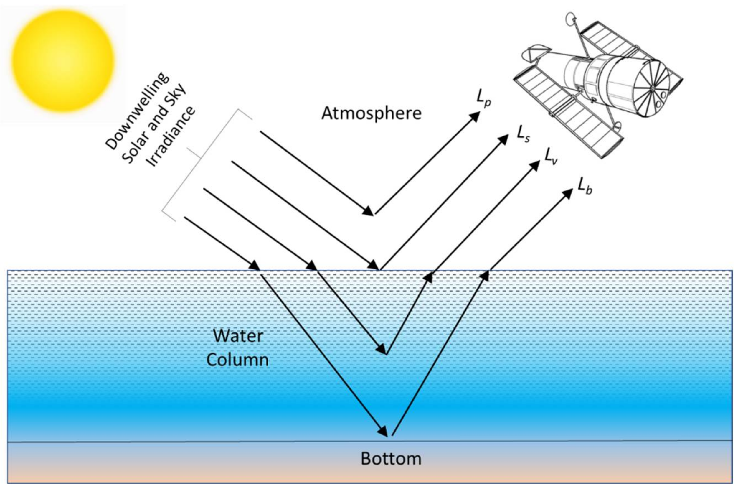
The total radiance (Lt), which is recorded by a remote sensing system over a waterbody, is a function of the electromagnetic energy from four different sources:
- 1.
Path radiance (Lp);
- 2.
Free-surface layer or boundary layer radiance (Ls);
- 3.
Subsurface volumetric radiance (Lv);
- 4.
Bottom radiance (Lb).
This is shown in Equation (1) and
Figure 1 [
8].
Path radiance (
Lp) is the radiance that is recorded by a sensor resulting from downwelling solar and sky radiation. This is usually unwanted as it never reaches the water. The free-surface layer or boundary layer radiance (
Ls) is the radiance that reaches the air–water interface. It only penetrates about 1 mm and is then reflected from the water surface. The spectral information about the near-surface characteristics of the water is contained in this reflected energy. The subsurface volumetric radiance (
Lv) is the radiance that penetrates the air–water interface and interacts with the organic/inorganic constituents in the water, and then exits the water column without encountering the bottom. It provides information about the internal bulk characteristics of the water column. The bottom radiance (
Lb) is the radiance that reaches the bottom of the waterbody, reflects from it, propagates back through the water column, and then exits the water column. This is useful to infer information about the bottom (e.g., depth, color) [
8].
The water-quality studies using remotely sensed data are usually interested in measuring the subsurface volumetric radiance (
Lv) exiting the water column toward the sensor. The characteristics of this radiant energy are a function of the concentration of pure water (
W), inorganic suspended minerals (
SM), organic chlorophyll
a (
Chl-a), dissolved organic material (
DOM), and the total amount of absorption and scattering attenuation that takes place in the water column due to each of these constituents,
c(
λ), as shown in Equation (2) [
8]:
It is important to look at the effect that each of these constituents has on the spectral reflectance characteristics of the water column. To estimate water quality parameters (WQPs) from different satellite data, three different approaches are generally used [
3,
4,
9]:
- 1.
Empirical approach, which is based on the development of bivariate or multivariate regressions between remote sensing data and measured in situ WQPs. Digital numbers (DN) or radiance values at the sensor, as well as their band combinations, are correlated with in situ measurements of different WQPs, usually acquired at near real-time of the sensor overpass. A summary of empirical approaches for lakes can be found in Lindell et al. [
10].
- 2.
Semi-empirical approach, which may be used when spectral characteristics of the parameters of interest are known. This knowledge of spectral characteristics is included in the statistical analysis by focusing on well-chosen spectral areas and appropriate spectral bands used as correlates. An example of a semi-empirical approach with different sensors is reported by Härmä et al. [
11], who investigated Finnish lakes.
- 3.
Analytical approach, where WQPs are related to the bulk Inherent Optical Properties (IOPs) via the Specific Inherent Optical Properties (SIOPs). The IOPs of the water column are then related to the Apparent Optical Properties (AOPs) and hence to the Top of Atmosphere (TOA) radiance, such as described by the radiative transfer theory [
12,
13]. The analytical method involves inverting the above-described relations to determine the WQPs from remote sensing data. An example of such an approach, using Landsat over lakes, can be found in Dekker et al. [
14] for the total suspended matter retrieval.
A recent comprehensive review on water quality remote sensing can be found in Gholizadeh et al. [
15], while a brief discussion on the current state of the art of the estimation of common WQPs using remote sensing is provided below.
1.1.1. Turbidity
Turbidity is a measure of water clarity derived from how much light is scattered by material in a body of water. Turbidity is a commonly assessed water quality parameter due to its optically active properties and was predicted as having high potential for correlation before satellite imagery was readily available [
16]. In the last four decades, quantitative predictions of turbidity, and other water transparency parameters, have been successfully carried out using spaceborne satellites in lacustrine, estuarine, reservoir, and coastal environments and validated against in situ measurements [
17,
18,
19,
20,
21,
22,
23,
24,
25,
26].
Satellites commonly used for deriving remotely sensed relationships with turbidity include Landsat 5, Landsat 8, and Sentinel-2 [
17,
18,
19,
20,
21,
24,
25,
26,
27,
28,
29]. Bands within the red and NIR wavelengths are most often chosen, either independently or combined with other bands, for developing these relationships [
17,
18,
19,
20,
21,
24,
25,
26,
27,
28,
29,
30,
31]. Green band wavelengths have been notably incorporated into ratios using multiple bands for turbidity analysis as well [
25,
29,
31].
Regression analyses with single or multi-band algorithms are common methods for assessing correlation between spectral reflectance and in situ turbidity measurements [
17,
18,
20,
21,
27,
30]. These methods are simple, efficient, and inexpensive for predicting water quality parameters with near-continuous spatial coverage. Other methods have found significant potential for correlation as well. Gene-expression programming (GEP) and geographically and temporally weighted regression (GTWR) have been proven to predict turbidity more accurately than that by multiple linear regression (MLR) among different reservoirs [
23,
26].
Beyond quantitative studies, qualitative studies are also common for prediction of turbidity when there are little to no in situ data available [
19,
29,
31]. These qualitative predictions can be useful for general assessment of water quality conditions when no quantitative predictions are necessary. For example, one study developed an index for qualitative analysis of turbidity, the Normalized Difference Turbidity Index (NDTI). This index used the green and red band reflectance values instead of in situ measurements and was successfully utilized during the COVID-19 pandemic when field sampling could not take place [
29,
31].
However, few studies have used spaceborne satellites to study turbidity in rivers. River waters, which contain inherent absorption and scattering properties, remain poorly understood. They consistently contribute to markedly greater error when they are correlated with spectral reflectance [
28]. Broad predictions of turbidity levels in rivers can still be made with statistically sound results when using specialized algorithms and regression models [
27,
28]. A qualitative assessment of fluvial turbidity was conducted by Greg et al. [
29].
1.1.2. Chlorophyll a (Chl-a)
Chl-
a is an optically active form of chlorophyll used in photosynthesis. It is one of the most studied remotely sensed water quality parameters. The majority of studies have found strongly correlated values detecting remotely sensed Chl-
a in lakes, reservoirs and coastal areas using data from Landsat 1–3, Landsat 5, Landsat 8, RapidEye, Sentinel-2, and MODIS satellites [
1,
5,
6,
20,
21,
32,
33,
34,
35,
36,
37,
38]. Successful correlations have also been found in past studies that utilized airborne remote sensing [
30,
39]. Limited success has been found in estuarine environments using imagery from Landsat 5 satellite and may need fine resolution imagery, as shown in [
19,
40] where IKONOS imagery was used.
An alternative way of assessing Chl-
a is by using the maximum chlorophyll index (MCI) which was developed to detect algal blooms specifically with MEdium Resolution Imaging Spectrometer (MERIS) imagery. Planet’s RapidEye satellite constellation was successfully used on lakes to create an equivalent product to that of MERIS detecting MCI [
1].
1.1.3. Suspended Sediment Concentration (SSC)
SSC values are derived by measuring the dry weight of sediment from a known volume of water. SSC has optically active properties that can be easily correlated against in situ measurements using regression analysis techniques. SSC has been successfully estimated in lacustrine, fluvial, and estuarine environments by several modern spaceborne sensors such as IKONOS, Landsat 8, Sentinel-2, RapidEye, and MODIS [
34,
40,
41,
42,
43,
44].
SSC has also been estimated using turbidity as a surrogate. There is a need to provide continuous records of SSC among ambient water gauge stations, particularly in polluted fluvial environments, as collecting in situ data is inefficient and costly [
45]. In situ turbidimeters are more practical and ubiquitous in water gauge stations and have proven to be a successful surrogate for indirectly measured SSC [
46,
47]. Many techniques have been published to reduce turbidity-derived SSC errors, including using artificial neural networks, calibrating turbidity estimates using remotely sensed imagery for seasonal variation differences, considering physical properties of SSC, and understanding the effects of hysteresis [
48,
49,
50,
51].
1.1.4. Total Suspended Solids (TSS)
TSS are optically active and they differ from SSC only by the differing laboratory analyses used to assess each. When compared to SSC, quantifying TSS has proven to be unreliable for samples measured from natural waters as methods were originally designed for analyzing wastewater [
52]. Regardless, TSS have been successfully estimated in lacustrine and estuarine environments using regression analysis techniques based on in situ measurements and reflectance data obtained from spaceborne optical sensors such as Landsat 5 and Landsat 8 [
5,
19,
20,
21]. Airborne remote sensing has been successful in assessing TSS of reservoirs and rivers, noting specific advantages over spaceborne satellites including less atmospheric interference, adaptable spatial resolution, and fewer temporal restraints [
30].
1.1.5. Salinity
Salinity is the total dissolved salt in water measured in parts per thousand. Salinity is known to be optically active, but there are also closely associated parameters, such as suspended solids, that can be used as a spectral surrogate in remote sensing studies [
19]. Lagerloef et al. [
53] presented a remote sensing salinity investigation prior to 1995 with early efforts using the dielectric constant of saline solutions as the physical basis for microwave remote sensing of ocean salinity. Airborne low frequency microwave radiometer experiments have shown success in measuring coastal surface salinity [
54]. Linear regression models are commonly used to estimate salinity in estuarine and coastal waters using imagery acquired by Landsat 5 and Landsat 8 satellites [
6,
19,
33,
55,
56].
1.1.6. Secchi Disk Depth (SDD)
SDD is a measure of water transparency, specifically the depth at which the opaque Secchi disk itself loses visibility from the surface. SDD has been successfully measured for decades via satellite and airborne remote sensing methods in a variety of environments including estuaries, rivers, reservoirs, and lakes. The most common method is to use varying techniques of regression analysis for predicting SDD as tested against in situ measurements [
20,
30,
32,
39,
40].
1.1.7. Total Dissolved Solids (TDS)
TDS are a measure of dissolved inorganic and organic substances in water and is related to electrical conductivity. TDS have been successfully estimated within lacustrine environments using regression techniques based on in situ measurements and reflectance data obtained from spaceborne optical sensors such as Landsat 5 and Landsat 8 [
21,
57].
1.1.8. Dissolved Oxygen (DO)
DO in a system is affected by many factors such as water temperature, respiring and decaying organisms, photosynthesizing plants, stream flow, and aeration. DO is optically inactive, but water temperature is a major influence of DO as oxygen more readily dissolves in cold water than in warm water. No sensor has been established to perform consistently accurate measurements of remotely sensed DO [
15]. A Landsat 5 TM-based study conducted by Qiu et al. achieved the best coefficient of determination (R
2) value of 0.68 by using a DO inversion exponential model [
58].
1.1.9. Dissolved Organic Carbon (DOC)
DOC is an optically inactive water quality parameter and few papers have been published attempting to predict DOC with satellite sensors against in situ data [
15]. Mapping dissolved organic carbon for inland waters through remote sensing was shown to be successful when utilizing common band ratio algorithms using Sentinel-2 imagery [
36]. DOC transport estimates along a fluvial environment were also found successful using a simple ratio algorithm using SeaWiFS imagery derived ocean color data [
59].
1.1.10. pH
It is not feasible to attain a direct correlation between surface reflectance and pH values, because pH is optically inactive [
15]. Using RapidEye imagery, Yigit Avdan et al. [
60] attempted to develop a model to predict pH by comparing in situ measurements and sensor reflectance values obtained over a lake but were unable to find any correlation among the data. Huang et al. [
61] developed a method to indirectly assess pH in water bodies through correlation with other water quality parameters such as salinity, temperature, and dissolved oxygen.
1.1.11. Total Nitrogen (TN) and Total Phosphorus (TP)
TN and TP concentrations in water are optically inactive. However, they have been estimated indirectly by correlating them with optically active chlorophyll
a, which was easily determined using Landsat 8 imagery [
62]. Older studies attempted to directly assess TP in lacustrine and estuarine environments using remotely sensed imagery (Landsat 1–3 and 5) correlated with in situ data to very limited success [
19,
32]. An anomalous paper found very high correlation values for both TN and TP using multiple regression analysis with in situ measurements and reflectance data obtained from Landsat 5 sensor [
57].
1.1.12. Colored Dissolved Organic Matter (CDOM)
CDOM is a large optically measurable portion of DOC. Inland bodies of water have high correlation values when assessing CDOM via remote sensing using a variety of sensors such as Sentinel-2, Landsat 8, and MODIS [
34,
36].
1.2. Objectives of the Current Study
Since no remote sensing-based algorithm is available to study surface water quality in the Tennessee River and its surrounding water bodies, the Geological and Environmental Remote Sensing Laboratory (GERS-Lab) at the University of Tennessee at Chattanooga recently started developing research programs to study surface water quality in the watersheds of Southeast Tennessee using satellite observations coupled with field measurements. As part of this initiative, this study’s objectives were twofold: first, conducting a comprehensive literature review on water quality remote sensing to develop a knowledge base about the state of the art of different water quality parameter estimation techniques using remotely sensed imagery, and second, developing models to estimate turbidity for the Tennessee River and its surrounding tributaries, taking the first step towards satellite observation-based water quality estimation model development for this area.
The literature review conducted in this study shows that turbidity is one of the most widely studied water quality parameters by remote sensing technology. Therefore, the objective of the current study is focused on the development of remote sensing-based numerical models to estimate turbidity for the Tennessee River and adjacent creeks. Landsat satellites are the most frequently used data sources for this purpose; thus, this study uses Landsat 8 Operational Land Imager (OLI) imagery coupled with concurrently acquired field measurements to develop the turbidity estimation models.
2. Materials and Methods
2.1. Study Site
The Tennessee River is the largest tributary of the Ohio River. It is approximately 1049 km long and is located in the southeastern United States within the Tennessee Valley [
63]. Its watershed is the fifth-largest in the nation, encompassing parts of six bordering states as well as Tennessee [
64]. The Tennessee River is formed at the confluence of the Holston River and the French Broad River in present-day Knoxville, Tennessee. From Knoxville, it flows southwest through East Tennessee into Chattanooga before crossing into Alabama. The Tennessee River defines the boundary between two of Tennessee’s grand divisions: Middle and West Tennessee [
63].
The Tennessee River is one of the most ecologically diverse rivers in the world and serves as a great resource for the residents living around it. However, it is also one of the most polluted rivers in the world [
64]. In fact, it is ranked as the fourth most polluted waterway in the United States [
65]. A leading cause of this pollution is storm water runoff. Runoff from rain and snow that consequently picks up fertilizers, insecticides, and other chemicals, such as phosphates (found in soap used to wash cars), carries these substances into wetlands and waterways, thereby polluting neighboring bodies of water such as the Tennessee River.
Water pollution from runoff subsequently causes concerns of eutrophication in the Tennessee River due to the nutrients that are loaded from urban areas. These excessive nutrients lead to algal blooms and ultimately result in a reduction of dissolved oxygen [
66]. This means that nutrients, such as nitrogen and phosphorous compounds needed for plant growth, mix with water in the Tennessee River by surface runoff, resulting in blooms of algal species [
67]. Algal blooms are concerning because their subsequent decay can produce an excessive oxygen demand resulting in bad odors, taste, and reduced oxygen levels, thereby harming other aquatic life [
67,
68]. Therefore, it is vital to explore the main source of pollution, storm water runoff, and its consequences such as eutrophication, the pollution’s effects on drinking water quality, and seek solutions to maintain a common resource, i.e., the Tennessee River.
The city of Chattanooga, TN, located along the Tennessee River, has grown substantially during the last several decades and has become the center of a series of urbanized sub-watersheds [
69]. Environmental impacts of this growth, especially the quality of surface waters, have become a major concern for the sustainable development of the greater Chattanooga areas [
69]. The successful development of a turbidity estimation algorithm would provide a powerful tool to aid in the study of the impacts of land use and land cover change on the surface water quality in the watersheds of Southeast Tennessee.
This study selected the part of the Tennessee River that flows through the city of Chattanooga as the study site. The selected site also includes a section of the South Chickamauga Creek adjacent to the Tennessee River.
Figure 2 shows the location and extent of the study site.
2.2. Data Collection
This study uses a time series of multispectral satellite imagery and concurrently acquired in situ water quality data. The description of the obtained data and the data acquisition techniques are briefly described below.
2.2.1. Satellite Imagery
The satellite images were obtained from the Landsat 8 mission. The images were acquired over the study site by the Operational Land Imager (OLI) sensor onboard the Landsat 8 satellite on 2 December 2018, 13 February 2019, and 15 August 2019. The imagery products were ordered and obtained through the U.S. Geological Survey (USGS) Earth Explorer. The Landsat 8 OLI Level-2 products, which provide the calculation of surface reflectance by the USGS, were used for spectral analysis. The characteristics of Landsat 8 imagery are provided in
Table 1.
Figure 3 and
Figures S1–S3 show the Landsat 8 OLI images acquired and used for this study.
2.2.2. Water Quality Data
In situ turbidity data were collected in different parts of the study site using a research vessel (a 16-foot-long Jon Boat) and a Hydrolab HL7 multiparameter sonde. This research specifically used the data acquired by the turbidity sensor on the sonde. The HL7 sensors were calibrated in the Geological and Environmental Remote Sensing Laboratory (GERS-Lab) at the University of Tennessee at Chattanooga (UTC) on the morning of field sampling. The calibration was done using the standard methods described in the Hydrolab operating software manual.
The data were collected concurrently with the Landsat imagery acquisition, which occurred on three dates: 2 December 2018, 13 February 2019, and 15 August 2019. Measurements were acquired at a total of 108 sample points across these three dates, with 35 samples on 2 December, 41 samples on 13 February, and 32 samples on 15 August.
Each sample was collected at similar depths within the water, extending about 20 cm from the surface. An individual sample was the average of 10 recordings for each parameter, collected at 1-second intervals. Parameter readings were stored in the Hydrolab Surveyor. The coordinates for each sample were collected concurrently using a Garmin eTrex 30x GPS unit. Hand-written records of each sample number, coordinates, and parameter values were also recorded in a field book.
Logged data files for the sample parameters were downloaded from the Hydrolab Surveyor using the supplied Hydrolab operating software. Downloaded data were imported into Microsoft Excel and associated with the GPS coordinates for further processing.
Figure 4 shows the distribution of sampling locations.
Table 2 provides the statistics of the acquired in situ turbidity measurements.
2.3. Turbidity Estimation Model Development
The turbidity estimation models developed in this study used an empirical approach based upon simple regressions between in situ measurements and surface reflectance data acquired by the Landsat 8 satellite mission. The statistical analyses were carried out using Microsoft Excel. The geospatial analyses were carried out using ESRI’s ArcGIS Pro software (versions 2.1–2.4). The simplicity of using single band regression models could create an avenue for developing routine turbidity estimations for the study site using Landsat 8 OLI satellite imagery. The flowchart in
Figure 5 shows the steps taken to build the turbidity model.
2.3.1. Data Pre-Processing
The acquired in situ turbidity measurements for all samples were separated by date, organized in a spreadsheet, and assigned unique Sample ID numbers beginning at and increasing sequentially by 1, with associated latitude and longitude coordinates in decimal degrees utilizing the WGS 1984 geographic coordinate system.
A point GIS data layer (shape file) was created for the locations of each date’s in situ turbidity measurements using the ‘XY Table to Point’ geoprocessing tool. The points are shown in
Figure 4.
All seven multispectral bands shown in
Table 1 were stacked together to prepare a seven-band multispectral composite image for each image acquired (
Figure 3 and
Figures S1–S3). The ‘Composite Bands’ geoprocessing tool was used to do this. Two scenes of Landsat 8 OLI images were available to cover the study site for 2 December 2018 and 15 August 2019. Both scenes were mosaicked using the ‘Mosaic to New Raster’ geoprocessing tool (
Figure 3,
Figures S1 and S3). There was only one scene available to cover the study site for 13 February 2019 (
Figure 3 and
Figure S2); therefore, mosaicking was not required for this date.
The scenes were then assessed and geo-rectified using ground control points. This was done to ensure positional accuracy, particularly along shorelines. Once each scene was correctly rectified, the pixels for land were then clipped to the USGS National Hydrography dataset of waterbodies, using the ‘Clip Raster’ tool. This removed extraneous pixels from land that would extend processing demands and improperly influence the water quality analysis.
The produced GIS point files for each set of in situ turbidity measurements were displayed on top of the processed multispectral images in true color corresponding to each date, i.e., 2 December 2018; sample points were overlayed upon imagery of the same date. This was done to identify the presence of any samples obscured by cloud coverage and proximity of stream banks. This way, only the measurements available without any influence of cloud and land could be selected for the model development. Due to this reason, three measurements from the December dataset and two measurements from the February dataset were removed from the final analysis. Seven measurements from the August dataset had to be removed since part of the image was covered by scattered clouds, as seen in
Figure 3 and
Figure S3. Finally, the total number of in situ turbidity measurements used for this study is 96, which includes 32, 39, and 25 measurements for December, February, and August image acquisitions, respectively.
2.3.2. Preparing Model Inputs
This study used the December and February datasets for both model development and testing. The August dataset was used exclusively for testing the model as a separate dataset without any influence in model development. The measurements for the December and February image acquisitions were divided into two sets: training and testing. The dataset used for training included 80% of the measurements whereas the dataset used for testing included 20% of the measurements. This provided 25 and 33 measurements for training the model using December and February image acquisitions, respectively. The dataset used for testing the model included 7 and 6 measurements for December and February image acquisitions, respectively. The selection of the measurements was done randomly using the ‘Subset Features’ geoprocessing tool available in the Geostatistical Analyst module in ArcGIS Pro software. As we can see in
Table 2, the turbidity measurements acquired in December did not have much statistical variation; however, the measurements acquired in February had more variation. Due to this, the datasets used for training the model for December and February image acquisitions were combined for model development. This made the total number of sample points used for training 58. All 25 measurements acquired during August image acquisition were used for further testing the model in addition to the datasets used for testing for December and February image acquisitions.
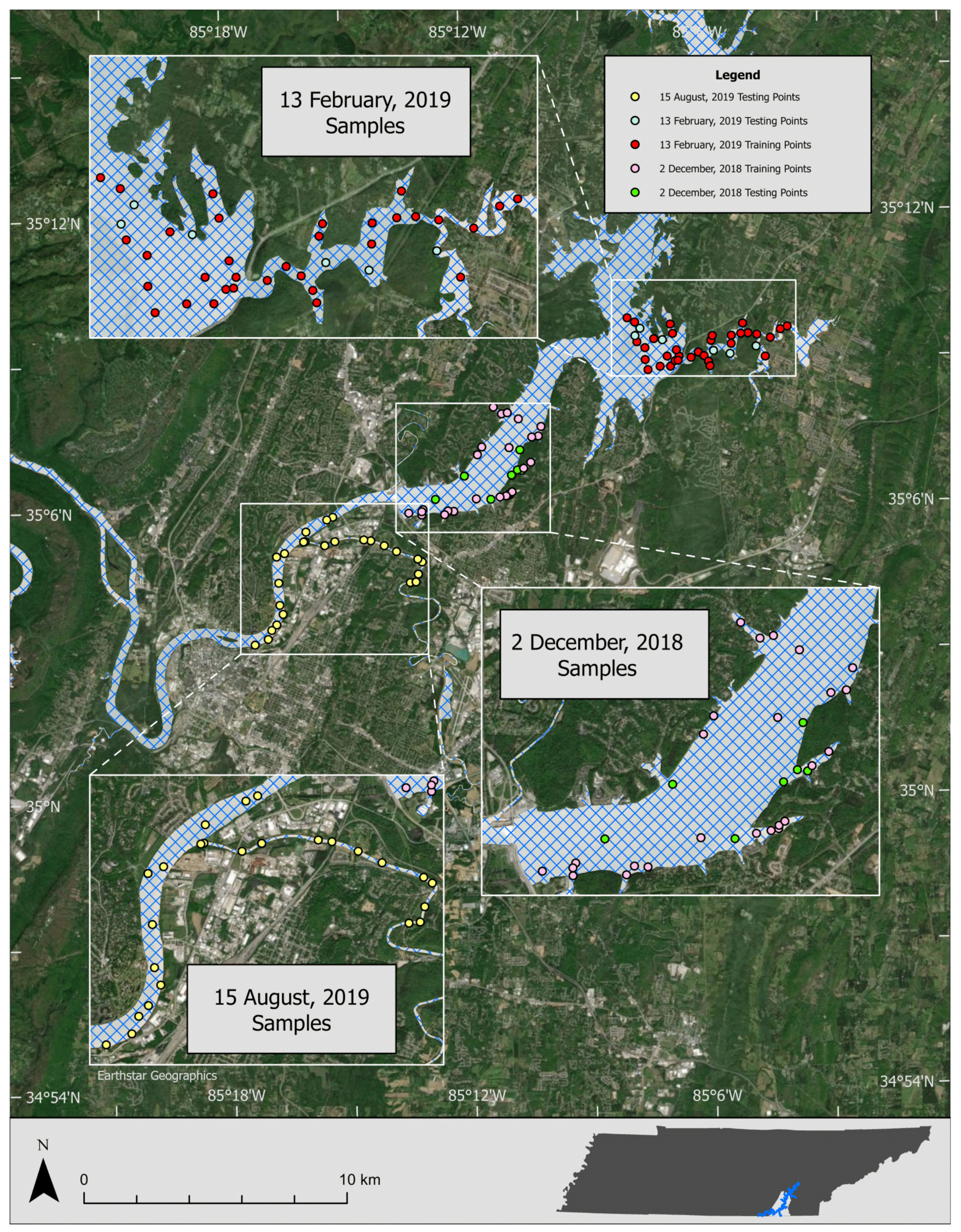
Figure 6 shows the distribution of the sample points used for training and testing for each date.
Spectral reflectance values were extracted using the ‘Extract Multi-Values to Points’ geoprocessing tool at the associated pixel for each sample’s coordinate location from each dataset used for training the model. This tool stores spectral reflectance for each spectral band, at each sample site, in the attribute table associated with each respective feature class. In order to conduct statistical analysis, the table for each respective feature class was converted to an Excel spreadsheet using the ‘Table to Excel’ tool.
Tables S1 and S2 show the extracted surface reflectance values for December and February image acquisitions.
2.3.3. Model Development
The extracted surface reflectance values (
Tables S1 and S2) from the sample points used for model training were exported to Microsoft Excel (Version 2108, Build 14326.20404) spreadsheets for conducting regression analysis. The ‘Table to Excel’ geoprocessing tool was used for this task. Single band exponential, power, and linear regressions for the dataset used for training were processed by generating scatter plots with spectral reflectance for each band on the x-axis plotted against corresponding in situ turbidity measurements on the y-axis. These regressions determined the spectral bands used as variables and corresponding equations for turbidity estimation. This also provided a value of coefficient of determination (R
2) associated with each best fit trend line used to determine the fit between the calculated regression line and the data.
Table 3 shows all the obtained regression equations and corresponding R
2 values.
Figure 7 shows the regression scatterplots for all bands (1–7).
The regression equations shown in
Table 3, scatterplots shown in
Figure 7, and the corresponding R
2 values were carefully assessed and the equation with the best R
2 value was selected to develop the model to estimate turbidity for the study site. The model was developed using the ‘ModelBuilder’ module available in ArcGIS Pro software. The ‘ModelBuilder’ module used several geoprocessing tools including ‘Make Raster Layer’ and ‘Raster Calculator’. The ‘Raster Calculator’ tool used the selected regression equation as algebraic expressions in Python, using the specific spectral bands as input variables (e.g., ρBand value). The output of this model was one raster, for each image acquisition date, which contained predicted turbidity values at each pixel of water within the study site.
2.3.4. Accuracy Assessment
The accuracy of the selected algorithm for turbidity estimation was assessed by using R
2 values and root mean square error (RMSE) values for each date from which the datasets used for model training were obtained. The corresponding test datasets, used for assessment of performance, are shown in
Table 4. The model’s capability to estimate turbidity during other Landsat 8 image acquisition was evaluated using the data collected on 15 August 2019 (
Table 5). The assessment was done using the obtained R
2 values and RMSE values. The R
2 values were calculated using the best fit line drawn on the scatterplots generated using the observed and predicted values. RMSE was calculated using the following equation:
where
N = number of samples used for accuracy assessment,
xi = observed values,
x′i = predicted values.
3. Results
Careful observations of all the regression equations (
Table 3), scatterplots (
Figure 7), and the corresponding R
2 values suggest that surface reflectance values recorded by Band 1 (Coastal), Band 2 (Blue), Band 3 (Green), and Band 4 (Red) are moderately to strongly correlated with the turbidity in the water of the study site as the majority of the obtained R
2 values range from 0.66 to 0.95. On the other hand, the surface reflectance values recorded by Band 5 (NIR), Band 6 (SWIR1), and Band 7 (SWIR2) are not well correlated with the turbidity in the water of the study site as the obtained R
2 values range from 0 to 0.44. For developing the turbidity estimation model, the nonlinear power regression (Equation (4)) that used Band 4 (Red) was selected since it achieved the highest value of R
2, 0.95:
where
T = Turbidity and ρ
red (Landsat 8) = Landsat 8 satellite red band surface reflectance values.
The Landsat scenes come packaged with Pixel Quality Assessment (QA) rasters that identify, among other classifications, cloud coverage and shadow, water, and land within a scene through an assigned value. The model-estimated turbidity pixels were extracted using a water mask prepared with the provided Landsat Pixel QA rasters. This water mask removed the influence of either clouds or both clouds and land. For visualization purposes, the masks that removed influence of both clouds and land were further clipped to the Tennessee River study site extent using the Tennessee River shapefile available in the GERS-Lab at UTC.
Figure 8 and
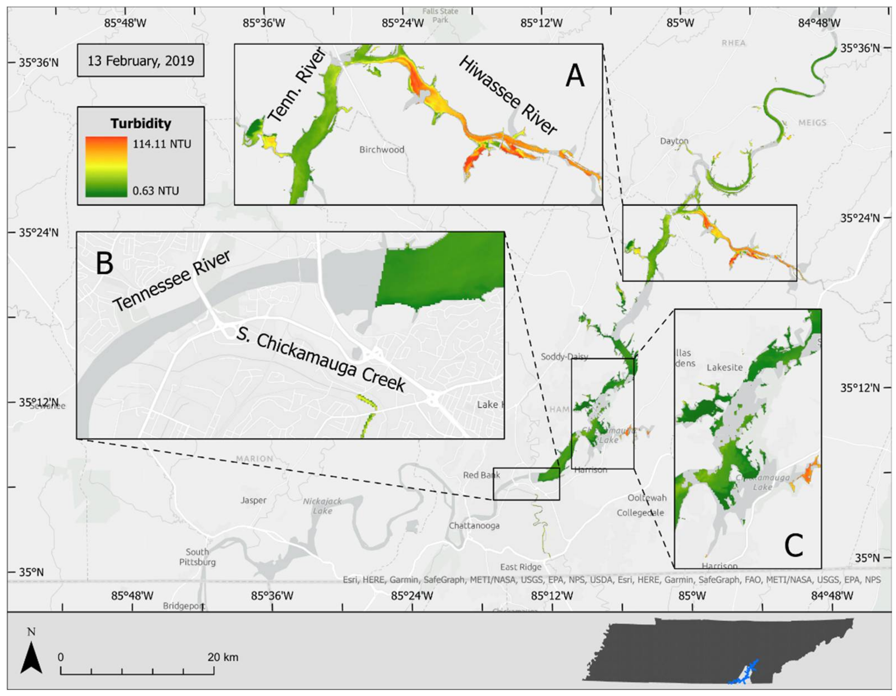
Figure 9 show the turbidity estimated on 2 December 2018 and 13 February 2019, respectively, by the model.
The model-derived turbidity estimation shows higher values of turbidity concentrated in the two major tributaries in the study site: South Chickamauga Creek and the Hiwassee River. This pattern was observed in both dates. However, the overall turbidity values were higher in February compared to those observed in December. Due to cloud coverage, it was not possible to estimate turbidity for the entire study site for the February image.
Using the test points shown in
Figure 6 and
Table 4, the predicted turbidity values were extracted from the newly created turbidity raster data for both February and December image acquisitions in order to perform accuracy assessments of the model. This was done by calculating the RMSE and R
2 of predicted values against the observed values. The RMSE values were calculated by Equation 3. The R
2 values were calculated by generating a best fit line on the scatterplots between the in situ turbidity measurements and corresponding estimated turbidity values. The scatterplots are shown in
Figure 10. The results are shown in
Table 6.
As shown in
Figure 10 and
Table 6, the turbidity estimation model performed better on the February image acquisition with a R
2 value of 0.97. The model only achieved a R
2 value of 0.31 for the December image acquisition. During image acquisition in February, a higher variation of turbidity values was observed; however, during image acquisition in December, a lower variation of turbidity values was observed (
Table 2). This difference appears to be what is causing inconsistency in model performance. Although the RMSE value for December was lower (1.414 NTU) compared to that of February (11.47 NTU), it can also be attributed to the nature of variation inherent to the acquired in situ turbidity measurements for these dates.
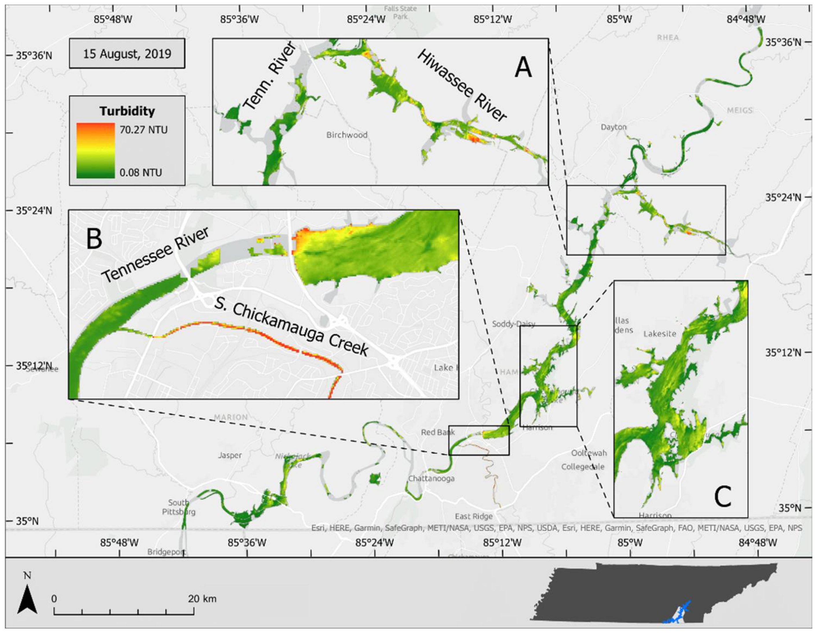
The turbidity estimation model’s performance was also assessed on a different date, 15 August 2019. This was done to see how the model performs on a Landsat 8 image for which no data are available for training the model. Equation 4 was applied on the processed surface reflectance values recorded by Band 4 (red) of the image acquired on 15 August 2019. The estimated turbidity image is shown in
Figure 11.
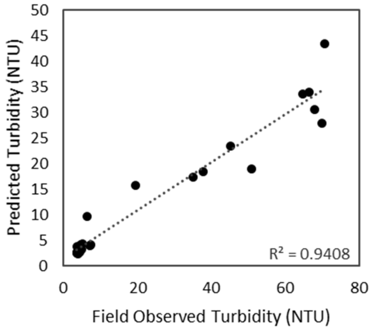
Using the test points shown in
Figure 6 and
Table 5, the predicted turbidity values were extracted from the newly created turbidity raster data for August image acquisition to perform accuracy assessments of the model. This was done by calculating RMSE and R
2 of predicted values against the observed values. The RMSE values were calculated by Equation 3. The R
2 values were calculated by generating a best fit line on the scatterplots between the observed test points and corresponding predicted turbidity values. The scatterplot is shown in
Figure 12. The results are shown in
Table 7.
Estimation of August turbidity provided results with generally high accuracy as evidenced by the obtained R
2 value of 0.94. The obtained RMSE value of 18.08 NTU was relatively higher than expected; however, this could be due to a few outliers present within the test point dataset as seen in
Figure 12.
4. Discussions
Ideally, in situ measurements would be obtained for the entire study site to improve the model accuracy, but this was not possible due to cloud coverage and limited resources. Consequently, this caused the data to be more skewed with less variation. Accuracy was improved by integrating the training data acquired during two field campaigns. However, since the test data were used separately, the difference of data variation influenced the results of accuracy assessments significantly. The test data with higher variation among observed values produced a higher R2 value and a higher RMSE value. Conversely, the test data with limited variation produced a lower R2 value and a lower RMSE value. This indicates that the availability of more in situ measurements and concurrent cloud free images would increase the consistency of model performance as it would then account for more variability. Therefore, it is strongly recommended to expand this research by incorporating more in situ measurements and concurrent image acquisitions.
Usually, it is desirable to acquire data for training and testing a model during both base flow and after a storm event to capture the variability of turbidity in stream water. However, due to cloud coverage issues and the image acquisition revisit calendar (Landsat 8 acquires images every 16 days) it is not always possible to achieve this. In this study it was possible to acquire training data after two similar precipitation events. The study site received rainfall in the amount of 20.32 mm and 33.27 mm on 1 December 2018, and 12 February 2019, respectively. The discharge values recorded during the time of image acquisition were 107.89 m3/s and 136.49 m3/s on 2 December 2018, and 13 February 2019, respectively. This provided the similar hydrologic conditions with the potential to have higher variability of turbidity concentrations. However, the availability of image and concurrent in situ measurements during the base flow conditions would increase the data variability further.
The study site received a very low amount of rainfall (1.02 mm) on the day before the image acquired (on 15 August 2019) for testing the model’s performance for routing turbidity estimation capacity. The recorded value of discharge during the image acquisition time was also very low, at 7.11 m3/s. This could be the reason for having higher RMSE values in the test results. So, it is recommended to perform this test again for the images acquired during similar hydrologic conditions comparing to the model’s training data. This would also provide us with the opportunity to see how different hydrologic conditions correlate with the remote-sensing-based turbidity estimations.
The majority of the remote-sensing-based inland turbidity studies are conducted in lacustrine environments. Spectral bands within the red and NIR wavelengths are most often chosen, either independently or combined with other bands, for developing turbidity estimation models [
17,
18,
19,
20,
21,
24,
25,
26,
27,
28,
29,
30,
31]. This study found that the red band performed the best for developing the model to estimate turbidity in the Tennessee River. The model achieved a R
2 value of 0.95. The models developed using the coastal, blue, and green bands also performed well for turbidity estimation. However, the models developed using the NIR band did not perform well as it did not show a strong relationship with turbidity. The obtained R
2 values were 0.16 to 0.44. This finding aligns with the study conducted by Lobo et al. [
27] in the Tapozos River Basin using Landsat MS/TM/OLI images. According to Lobo et al. [
27], when water turbidity is high, suspended particles are easily detected by the NIR spectrum. However, higher content of clay particles in water may increase the surface reflectance of the red spectrum compared to sand-rich waters. On the other hand, surface reflectance values should be close to zero in NIR channels for perfectly clear waters. However, in narrow water channels, adjacency of land can erroneously increase NIR surface reflectance, especially in the case for satellites with a low spatial resolution. The visible bands are largely unaffected by this adjacency influence. Therefore, it is suggested to avoid using the NIR band to derive turbidity in narrow fluvial environments for this reason. Since the study site of this research includes narrow fluvial environments, it is possible to have similar issues described by Lobo et al. [
27] with NIR bands. More investigations are needed to draw conclusions in this regard.
This research aimed to develop a turbidity estimation model using a single band to simplify the regression equation and to make it suitable for easier implementation of the model for routing operation. However, since other studies [
17,
18,
20,
21,
27,
30] showed success in using multiple bands for turbidity estimation, those methods should also be explored in the future for this area.
Strong winds can generate waves and cause variation in surface water turbidity. However, this is expected not to have any significant influence on the overall surface reflectance values since one pixel of a Landsat 8 image covers about 900 m2 on the ground. Surface reflectance values recorded by one pixel is the average of the reflectance values recorded over an area of 900 m2.
5. Conclusions
Remote sensing technology has been used successfully for water quality estimation for many years. Turbidity is one of the most frequently used water quality parameters that can be estimated from remote sensing, with Landsat satellites being the most widely used spaceborne technology in this regard.
Currently, no remote-sensing-based water quality estimation model is available for the Tennessee River, albeit it being one of the most ecologically diverse and polluted rivers in the world. This research developed a turbidity estimation model using imagery from the Landsat 8 satellite mission, providing us with the opportunity to estimate turbidity in the Tennessee River every 16 days at a 30 m spatial resolution.
At present, there are only a few scattered water quality measuring stations in the Tennessee River and its surrounding tributaries. With this limited water quality measuring capability, it is very challenging or even impossible for some areas to adequately study the water quality in this area. The model developed by this study using Landsat 8 satellite imagery would provide with the turbidity estimation capability in the Tennessee River and its surrounding tributaries at every 900 m2 surface area. This can be acquired whenever a cloud-free Landsat 8 OLI image is available.
As the city of Chattanooga, TN is being continuously urbanized, the environmental impacts, especially the quality of surface waters due to this growth, have become a major concern for the sustainable development of the greater Chattanooga area [
69]. This remote-sensing-based turbidity estimation model would be very useful to monitor turbidity in the Tennessee River and its surrounding tributaries throughout the year.
The results obtained in this study indicate that a simple nonlinear regression-based model could be developed using the surface reflectance values recorded in Band 4 (red) of the Landsat 8 OLI sensor to estimate turbidity in the Tennessee River and its tributaries. This is strongly supported by the obtained R
2 values for model development (
Table 3 and
Figure 7). The accuracy assessments of the estimated turbidity images (
Figure 8 and
Figure 9) also indicate promising prospects in this regard, as the highest R
2 value was 0.97 and the lowest RMSE was 1.414 NTU (
Table 6).
The model was also tested to evaluate its potential for routine operational use for turbidity estimation in the Tennessee River and its tributaries. The test results were promising as the obtained R2 and RMSE values were 0.94 and 18.01 NTU, respectively. However, since the model was only tested on one image acquisition date, 15 August 2019, it would be beneficial to test this model on data acquired from other image acquisition dates with near real-time in situ turbidity measurements.
Supplementary Materials
The following are available online at
https://www.mdpi.com/article/10.3390/rs13183785/s1, Figure S1: One of three Landsat 8 OLI images acquired over the study site on 2 December 2018. The image is subset to the study site extent displayed in true color. The inset regions represent areas of high turbidity variability due to the convergence of lakes and minor streams with the Tennessee River, Figure S2: One of three Landsat 8 OLI images acquired over the study site on 13 February 2019. The image is subset to the study site extent displayed in true color. The inset regions represent areas of high turbidity variability due to the convergence of lakes and minor streams with the Tennessee River, Figure S3: One of three Landsat 8 OLI images acquired over the study site on 15 August 2019. The image is subset to study site extent displayed in true color. The inset regions represent areas of high turbidity variability due to the convergence of lakes and minor streams with the Tennessee River, Table S1: Model training data for 2 December 2018 image acquisition, Table S2: Model training data for 13 February 2019 image acquisition.
Author Contributions
Conceptualization, A.K.M.A.H.; Data curation, A.K.M.A.H., C.M. and R.B.; Investigation, A.K.M.A.H., C.M. and R.B.; Methodology, A.K.M.A.H. and C.M.; Formal analysis, C.M. and R.B.; Project administration, A.K.M.A.H.; Supervision, A.K.M.A.H.; Validation, C.M.; Writing—original draft, A.K.M.A.H. and C.M.; Writing—review & editing, A.K.M.A.H., C.M. and R.B.; Funding acquisition, A.K.M.A.H. All authors have read and agreed to the published version of the manuscript.
Funding
This research was funded by the Center of Excellence in Applied Computational Science and Engineering grants program at the University of Tennessee at Chattanooga. This research was also funded by the Faculty Prep Grant, the Office of Research and Sponsored Program, and the Department of Biology, Geology, and Environmental Science at the University of Tennessee at Chattanooga.
Institutional Review Board Statement
This is not relevant to this study.
Informed Consent Statement
This is not relevant to this study.
Data Availability Statement
Some of the data are already provided in the
supplementary materials section of this publication. Other data presented in this study are available on request from the corresponding author.
Acknowledgments
The authors thankfully acknowledge the support from the Office of Research and Sponsored Program, the Center of Excellence in Applied Computational Science and Engineering, the Department of Biology, Geology and Environmental Science, and the SimCenter at the University of Tennessee at Chattanooga. Thanks are also due to NASA/USGS for providing the Landsat 8 satellite imagery free of charge. The authors would like to thank Mark Schorr and Jejal Bathi for their help to plan the field data acquisition for this research. Special thanks are due to William Adair for his valuable help in the field for acquiring in situ turbidity measurements. A special thanks is due to John Tucker for his help and support for the research vessel used in the field.
Conflicts of Interest
The authors declare no conflict of interest. The funders had no role in the design of the study; in the collection, analyses, or interpretation of data; in the writing of the manuscript, or in the decision to publish the results.
References
- Mishra, S.; Stumpf, R.P.; Meredith, A. Evaluation of RapidEye data for mapping algal blooms in inland waters. Int. J. Remote Sens. 2019, 40, 2811–2829. [Google Scholar] [CrossRef]
- Wu, M.; Zhang, W.; Wang, X.; Luo, D. Application of MODIS satellite data in monitoring water quality parameters of Chaohu Lake in China. Environ. Monit. Assess. 2009, 148, 255–264. [Google Scholar] [CrossRef]
- Cracknell, A.; Newcombe, S.; Black, A.; Kirby, N. The ABDMAP (algal bloom detection, monitoring and prediction) concerted action. Int. J. Remote Sens. 2001, 22, 205–247. [Google Scholar] [CrossRef]
- Dekker, A.G.; Malthus, T.J.; Hoogenboom, H.J. The remote sensing of inland water quality. In Advances in Environmental Remote Sensing; Danson, F.M., Plummer, S.E., Eds.; John Wiley & Sons Ltd: Hoboken, NJ, USA, 1995; pp. 123–142. [Google Scholar]
- Hossain, A.K.M.A.; Jia, Y.; Chao, X. Development of Remote Sensing Based Index for Estimating/Mapping Suspended Sediment Concentration in River and Lake Environments. In Proceedings of the 8th International Symposium on Ecohydraulics (ISE 2010), Seoul, Korea, 12–16 September 2010; pp. 578–585. [Google Scholar]
- Hossain, A.K.M.A.; Jia, Y.; Chao, X.; Altinakar, M. Application of advanced remote sensing techniques to improve modeling estuary water quality. In Remote Sensing and Modeling; Springer: Berlin, Germany, 2014; pp. 295–313. [Google Scholar]
- Hossain, A.K.M.A.; Chao, X.; Cizdziel, J.; Jia, Y.; Altinakar, A. Exploring the Potential of Remote Sensing Techniques for Quantitative Estimation of Mercury Concentration in Inland Surface Water Bodies. In Proceedings of the ASPRS Annual Conference—Imaging & Geospatial Technology Forum (IGTF), Baltimore, MD, USA, 12–16 March 2017. [Google Scholar]
- Jensen, J.R. Remote Sensing of the Environment: An Earth Resource Perspective, 2nd ed.; Pearson: London, UK, 2006; p. 592. [Google Scholar]
- Ambarwulan, W.; Salama, M.; Mannaerts, C.; Verhoef, W. Estimating specific inherent optical properties of tropical coastal waters using bio-optical model inversion and in situ measurements: Case of the Berau estuary, East Kalimantan, Indonesia. Hydrobiologia 2011, 658, 197–211. [Google Scholar] [CrossRef] [Green Version]
- Lindell, T.; Pierson, D.; Premazzi, G. Manual for Monitoring European Lakes Using Remote Sensing Techniques; Joint Research Centre: Ispra, Italy, 1999. [Google Scholar]
- Härmä, P.; Vepsäläinen, J.; Hannonen, T.; Pyhälahti, T.; Kämäri, J.; Kallio, K.; Eloheimo, K.; Koponen, S. Detection of water quality using simulated satellite data and semi-empirical algorithms in Finland. Sci. Total Environ. 2001, 268, 107–121. [Google Scholar] [CrossRef]
- Mobley, C.D.; Mobley, C.D. Light and Water: Radiative Transfer in Natural Waters; Academic Press: Cambridge, MA, USA, 1994. [Google Scholar]
- Vermote, E.; Tanré, D.; Deuzé, J.; Herman, M.; Morcrette, J.; Kotchenova, S. Second simulation of a satellite signal in the solar spectrum-vector (6SV). 6S User Guide Version 2006, 3, 1–55. [Google Scholar]
- Dekker, A.; Vos, R.; Peters, S. Comparison of remote sensing data, model results and in situ data for total suspended matter (TSM) in the southern Frisian lakes. Sci. Total Environ. 2001, 268, 197–214. [Google Scholar] [CrossRef]
- Gholizadeh, M.H.; Melesse, A.M.; Reddi, L. A comprehensive review on water quality parameters estimation using remote sensing techniques. Sensors 2016, 16, 1298. [Google Scholar] [CrossRef] [Green Version]
- Moore, G.K. Satellite remote sensing of water turbidity/Sonde de télémesure par satellite de la turbidité de l′eau. Hydrol. Sci. Bull. 1980, 25, 407–421. [Google Scholar] [CrossRef]
- Harrington, J.A., Jr.; Schiebe, F.R.; Nix, J.F. Remote sensing of Lake Chicot, Arkansas: Monitoring suspended sediments, turbidity, and Secchi depth with Landsat MSS data. Remote Sens. Environ. 1992, 39, 15–27. [Google Scholar] [CrossRef]
- Lathrop, R.G. Landsat Thematic Mapper monitoring of turbid inland water quality. Photogramm. Eng. Remote Sens. 1992, 58, 465–470. [Google Scholar]
- Baban, S.M.J. Environmental monitoring of estuaries; estimating and mapping various environmental indicators in Breydon Water Estuary, UK, using Landsat TM imagery. Estuar. Coast. Shelf Sci. 1997, 44, 589–598. [Google Scholar] [CrossRef]
- Wang, F.; Han, L.; Kung, H.T.; Van Arsdale, R.B. Applications of Landsat-5 TM imagery in assessing and mapping water quality in Reelfoot Lake, Tennessee. Int. J. Remote Sens. 2006, 27, 5269–5283. [Google Scholar] [CrossRef]
- Al-Fahdawi, A.A.H.; Rabee, A.M.; Al-Hirmizy, S.M. Water quality monitoring of Al-Habbaniyah Lake using remote sensing and in situ measurements. Environ. Monit. Assess. 2015, 187, 367. [Google Scholar] [CrossRef] [PubMed]
- Dörnhöfer, K.; Oppelt, N. Remote sensing for lake research and monitoring—Recent advances. Ecol. Indic. 2016, 64, 105–122. [Google Scholar] [CrossRef]
- Chu, H.-J.; Kong, S.-J.; Chang, C.-H. Spatio-temporal water quality mapping from satellite images using geographically and temporally weighted regression. Int. J. Appl. Earth Obs. Geoinf. 2018, 65, 1–11. [Google Scholar] [CrossRef]
- Rudorff, N.; Rudorff, C.M.; Kampel, M.; Ortiz, G. Remote sensing monitoring of the impact of a major mining wastewater disaster on the turbidity of the Doce River plume off the eastern Brazilian coast. ISPRS J. Photogramm. Remote Sens. 2018, 145, 349–361. [Google Scholar] [CrossRef]
- Surisetty, V.V.A.K.; Sahay, A.; Ramakrishnan, R.; Samal, R.N.; Rajawat, A.S. Improved turbidity estimates in complex inland waters using combined NIR–SWIR atmospheric correction approach for Landsat 8 OLI data. Int. J. Remote Sens. 2018, 39, 7463–7482. [Google Scholar] [CrossRef]
- Liu, L.-W.; Wang, Y.-M. Modelling reservoir turbidity using Landsat 8 satellite imagery by gene expression programming. Water 2019, 11, 1479. [Google Scholar] [CrossRef] [Green Version]
- Lobo, F.L.; Costa, M.P.F.; Novo, E.M.L.M. Time-series analysis of Landsat-MSS/TM/OLI images over Amazonian waters impacted by gold mining activities. Remote Sens. Environ. 2015, 157, 170–184. [Google Scholar] [CrossRef]
- Kuhn, C.; de Matos Valerio, A.; Ward, N.; Loken, L.; Sawakuchi, H.O.; Kampel, M.; Richey, J.; Stadler, P.; Crawford, J.; Striegl, R.; et al. Performance of Landsat-8 and Sentinel-2 surface reflectance products for river remote sensing retrievals of chlorophyll-a and turbidity. Remote Sens. Environ. 2019, 224, 104–118. [Google Scholar] [CrossRef] [Green Version]
- Garg, V.; Aggarwal, S.P.; Chauhan, P. Changes in turbidity along Ganga River using Sentinel-2 satellite data during lockdown associated with COVID-19. Geomat. Nat. Hazards Risk 2020, 11, 1175–1195. [Google Scholar] [CrossRef]
- Dierberg, F.E.; Carriker, N.E. Field testing two instruments for remotely sensing water quality in the Tennessee Valley. Environ. Sci. Technol. 1994, 28, 16–25. [Google Scholar] [CrossRef] [PubMed]
- Lacaux, J.P.; Tourre, Y.M.; Vignolles, C.; Ndione, J.A.; Lafaye, M. Classification of ponds from high-spatial resolution remote sensing: Application to Rift Valley Fever epidemics in Senegal. Remote Sens. Environ. 2007, 106, 66–74. [Google Scholar] [CrossRef]
- Garrison, V.; Bryant, N. Lake classification in Vermont. In Proceedings of the 2nd Eastern Regional Remote Sensing Applications Conference (US NASA, Goddard Space Flight Center, NASA CP 2198), Greenbelt, MD, USA, 18–22 May 1981; pp. 345–351. [Google Scholar]
- Chao, X.; Jia, Y.; Hossain, A.K.M.A.; Zhang, Y. Numerical simulation of sediment transport, phytoplankton biomass and salinity recovery processes in Lake Pontchartrain due to Bonnet Carré Spillway flood release. Ecol. Eng. 2021, 160, 106151. [Google Scholar] [CrossRef]
- Giardino, C.; Bresciani, M.; Cazzaniga, I.; Schenk, K.; Rieger, P.; Braga, F.; Matta, E.; Brando, V.E. Evaluation of multi-resolution satellite sensors for assessing water quality and bottom depth of Lake Garda. Sensors 2014, 14, 24116–24131. [Google Scholar] [CrossRef] [PubMed] [Green Version]
- Keith, D.; Rover, J.; Green, J.; Zalewsky, B.; Charpentier, M.; Thursby, G.; Bishop, J. Monitoring algal blooms in drinking water reservoirs using the Landsat-8 Operational Land Imager. Int. J. Remote Sens. 2018, 39, 2818–2846. [Google Scholar] [CrossRef] [PubMed]
- Toming, K.; Kutser, T.; Laas, A.; Sepp, M.; Paavel, B.; Nõges, T. First experiences in mapping lake water quality parameters with Sentinel-2 MSI imagery. Remote Sens. 2016, 8, 640. [Google Scholar] [CrossRef] [Green Version]
- Vanhellemont, Q.; Ruddick, K. Acolite for Sentinel-2: Aquatic Applications of MSI imagery. In Proceedings of the 2016 ESA Living Planet Symposium, Prague, Czech Republic, 9–13 May 2016; pp. 9–13. [Google Scholar]
- Chen, Y.; Wang, Y.; Xie, T.; Zhang, M. Analysis for the Change of Aquaculture Area and Water Quality in Sansha Bay During 2010–2018. In Proceedings of the IGARSS 2019—2019 IEEE International Geoscience and Remote Sensing Symposium, Yokohama, Japan, 28 July–2 August 2019; pp. 8264–8267. [Google Scholar]
- Dekker, A.G.; Zamurović-Nenad, Ž.; Hoogenboom, H.J.; Peters, S.W.M. Remote sensing, ecological water quality modelling and in situ measurements: A case study in shallow lakes. Hydrol. Sci. J. 1996, 41, 531–547. [Google Scholar] [CrossRef]
- Ekercin, S. Water quality retrievals from high resolution IKONOS multispectral imagery: A case study in Istanbul, Turkey. Water Air Soil Pollut. 2007, 183, 239–251. [Google Scholar] [CrossRef]
- Tsapanou, A.; Oikonomou, E.; Drakopoulos, P.; Poulos, S.; Sylaios, G. Coupling remote sensing data with in-situ optical measurements to estimate suspended particulate matter under the Evros river influence (North-East Aegean Sea, Greece). Int. J. Remote Sens. 2019, 41, 1–19. [Google Scholar] [CrossRef]
- Wu, G.; Cui, L.; Liu, L.; Chen, F.; Fei, T.; Liu, Y. Statistical model development and estimation of suspended particulate matter concentrations with Landsat 8 OLI images of Dongting Lake, China. Int. J. Remote Sens. 2015, 36, 343–360. [Google Scholar] [CrossRef]
- Liu, H.; Li, Q.; Shi, T.; Hu, S.; Wu, G.; Zhou, Q. Application of sentinel 2 MSI images to retrieve suspended particulate matter concentrations in Poyang Lake. Remote Sens. 2017, 9, 761. [Google Scholar] [CrossRef] [Green Version]
- Pereira, F.J.S.; Costa, C.A.G.; Foerster, S.; Brosinsky, A.; de Araújo, J.C. Estimation of suspended sediment concentration in an intermittent river using multi-temporal high-resolution satellite imagery. Int. J. Appl. Earth Obs. Geoinf. 2019, 79, 153–161. [Google Scholar] [CrossRef]
- Gray, J.R.; Gartner, J.W. Technological advances in suspended-sediment surrogate monitoring. Water Resour. Res. 2009, 45. [Google Scholar] [CrossRef] [Green Version]
- Ellison, C.A.; Savage, B.E.; Johnson, G.D. Suspended-sediment concentrations, loads, total suspended solids, turbidity, and particle-size fractions for selected rivers in Minnesota, 2007 through 2011. US Geol. Surv. Sci. Invest. Rep. 2014, 5, 43. [Google Scholar]
- Teixeira, L.C.; de Paiva, J.B.D.; da Silva Pereira, J.E.; de Moura Lisbôa, R. Relationship between turbidity and suspended sediment concentration from a small hydrographic basin in Santa Maria (Rio Grande do Sul, Brazil). Int. J. River Basin Manag. 2016, 14, 393–399. [Google Scholar] [CrossRef]
- Bayram, A.; Kankal, M.; Önsoy, H. Estimation of suspended sediment concentration from turbidity measurements using artificial neural networks. Environ. Monit. Assess. 2012, 184, 4355–4365. [Google Scholar] [CrossRef] [PubMed]
- Jafar-Sidik, M.; Gohin, F.; Bowers, D.; Howarth, J.; Hull, T. The relationship between Suspended Particulate Matter and Turbidity at a mooring station in a coastal environment: Consequences for satellite-derived products. Oceanologia 2017, 59, 365–378. [Google Scholar] [CrossRef]
- Jastram, J.D.; Zipper, C.E.; Zelazny, L.W.; Hyer, K.E. Increasing precision of turbidity-based suspended sediment concentration and load estimates. J. Environ. Qual. 2010, 39, 1306–1316. [Google Scholar] [CrossRef]
- Landers, M.N.; Sturm, T.W. Hysteresis in suspended sediment to turbidity relations due to changing particle size distributions. Water Resour. Res. 2013, 49, 5487–5500. [Google Scholar] [CrossRef]
- Gray, J.R.; Glysson, G.D.; Turcios, L.M.; Schwarz, G.E. Comparability of Suspended-Sediment Concentration and Total Suspended Solids Data; No. 4191; US Department of the Interior, US Geological Survey: Reston, VA, USA, 2000.
- Lagerloef, G.S.; Swift, C.T.; Le Vine, D.M. Sea surface salinity: The next remote sensing challenge. Oceanography 1995, 8, 44–50. [Google Scholar] [CrossRef]
- D′sa, E.J.; Zaitzeff, J.B.; Steward, R.G. Monitoring water quality in Florida Bay with remotely sensed salinity and in situ bio-optical observations. Int. J. Remote Sens. 2000, 21, 811–816. [Google Scholar] [CrossRef]
- Zhao, J.; Temimi, M.; Ghedira, H. Remotely sensed sea surface salinity in the hyper-saline Arabian Gulf: Application to Landsat 8 OLI data. Estuar. Coast. Shelf Sci. 2017, 187, 168–177. [Google Scholar] [CrossRef] [Green Version]
- Wang, F.; Xu, Y.J. Development and application of a remote sensing-based salinity prediction model for a large estuarine lake in the US Gulf of Mexico coast. J. Hydrol. 2008, 360, 184–194. [Google Scholar] [CrossRef]
- Coskun, H.G.; Tanik, A.; Alganci, U.; Cigizoglu, H.K. Determination of environmental quality of a drinking water reservoir by remote sensing, GIS and regression analysis. Water Air Soil Pollut. 2008, 194, 275–285. [Google Scholar] [CrossRef]
- Qiu, Y.; Zhang, H.E.; Tong, X.; Zhang, Y.; Zhao, J. Monitoring the Water Quality of Water Resources Reservation Area in Upper Region of Huangpu River using Remote Sensing. In Proceedings of the 2006 IEEE International Symposium on Geoscience and Remote Sensing, Denver, CO, USA, 31 July–4 August 2006; pp. 1082–1085. [Google Scholar]
- Del Castillo, C.E.; Miller, R.L. On the use of ocean color remote sensing to measure the transport of dissolved organic carbon by the Mississippi River Plume. Remote Sens. Environ. 2008, 112, 836–844. [Google Scholar] [CrossRef] [Green Version]
- Yigit Avdan, Z.; Kaplan, G.; Goncu, S.; Avdan, U. Monitoring the water quality of small water bodies using high-resolution remote sensing data. ISPRS Int. J. Geoinf. 2019, 8, 553. [Google Scholar] [CrossRef] [Green Version]
- Huang, H.; Feng, R.; Zhu, J.; Li, P. Prediction of pH value by multi-classification in the Weizhou Island area. Sensors 2019, 19, 3875. [Google Scholar] [CrossRef] [Green Version]
- Vakili, T.; Amanollahi, J. Determination of optically inactive water quality variables using Landsat 8 data: A case study in Geshlagh reservoir affected by agricultural land use. J. Clean. Prod. 2019, 247, 119134. [Google Scholar] [CrossRef]
- Navigation on the Tennessee River. Available online: https://www.tva.com/Environment/Managing-the-River/Navigation-on-the-Tennessee-River (accessed on 11 August 2021).
- Tennessee’s Dangerous Waters. Available online: https://www.nytimes.com/2019/10/28/opinion/tennessees-dangerous-waters.html (accessed on 11 August 2019).
- Sharp, R.; Pestano, P. Water Treatment Contaminants: Forgotten Toxics in American Water. Available online: https://static.ewg.org/reports/2013/water_filters/2013_tap_water_report_final.pdf (accessed on 11 August 2021).
- Robbins, P.; Hintz, J.; Moore, S.A. Environment and Society: A Critical Introduction; John Wiley & Sons: Hoboken, NJ, USA, 2014. [Google Scholar]
- Hampson, P.S.; Treece, M.; Johnson, G.C.; Ahlstedt, S.; Connell, J.F. Water Quality in the Upper Tennessee River Basin, Tennessee, North Carolina, Virginia, and Georgia, 1994–1998; US Geological Survey: Reston, VA, USA, 2000; Volume 1205.
- Rodriguez, V. Knoxville water pollution remains a concern for professionals, environmental groups. Available online: https://tnjn.com/blog/2017/04/20/knoxville-water-pollution-remains-a-concern-for-professionals-environmental-groups/ (accessed on 11 August 2021).
- Hall, J.; Hossain, A.K.M.A. Mapping urbanization and evaluating its possible impacts on stream water quality in Chattanooga, Tennessee, using GIS and remote sensing. Sustainability 2020, 12, 1980. [Google Scholar] [CrossRef] [Green Version]
Figure 1.
Remote sensing of water quality (modified from [
8]).
Figure 1.
Remote sensing of water quality (modified from [
8]).
Figure 2.
Map showing the location and extent of the study site, the Tennessee River and its surrounding tributaries.
Figure 2.
Map showing the location and extent of the study site, the Tennessee River and its surrounding tributaries.
Figure 3.
Landsat 8 OLI images acquired over the study site on 2 December 2018, 13 February 2019, and 15 August 2019.
Figure 3.
Landsat 8 OLI images acquired over the study site on 2 December 2018, 13 February 2019, and 15 August 2019.
Figure 4.
Location of in situ turbidity samples collected on each of the three dates for which Landsat 8 satellite images were acquired.
Figure 4.
Location of in situ turbidity samples collected on each of the three dates for which Landsat 8 satellite images were acquired.
Figure 5.
Flowchart illustrates the workflow followed in development of the model.
Figure 5.
Flowchart illustrates the workflow followed in development of the model.
Figure 6.
Map showing the locations of in situ turbidity samples collected on each of the three dates, separated into the sample points used for training and testing the model.
Figure 6.
Map showing the locations of in situ turbidity samples collected on each of the three dates, separated into the sample points used for training and testing the model.
Figure 7.
Regression scatterplots for all bands: linear regressions (left); nonlinear exponential regressions (middle); nonlinear power regressions (right).
Figure 7.
Regression scatterplots for all bands: linear regressions (left); nonlinear exponential regressions (middle); nonlinear power regressions (right).
Figure 8.
Turbidity estimated on 2 December 2018 by the turbidity estimation model. The insets highlight areas of high turbidity variability due to the convergence of lakes and streams. Site A details the confluence of the Tennessee and Hiwassee Rivers, Site B highlights the increased turbidity of South Chickamauga Creek, and Site C details the Harrison Bay area.
Figure 9.
Turbidity estimated on 13 February 2019 by the turbidity estimation model. The insets highlight areas of high turbidity variability due to the convergence of lakes and streams. Site A details the confluence of the Tennessee and Hiwassee Rivers, Site B highlights the increased turbidity of South Chickamauga Creek, and Site C details the Harrison Bay area.
Figure 10.
Scatterplots illustrating the relationship between the predicted and observed turbidity values for 2 December 2018 (left) and 13 February 2019 (right).
Figure 10.
Scatterplots illustrating the relationship between the predicted and observed turbidity values for 2 December 2018 (left) and 13 February 2019 (right).
Figure 11.
Turbidity estimated on 15 August 2019 by the turbidity estimation model. The insets highlight areas of high turbidity variability due to the convergence of lakes and streams. Site A details the confluence of the Tennessee and Hiwassee Rivers, Site B highlights the increased turbidity of South Chickamauga Creek, and Site C details the Harrison Bay area.
Figure 12.
Scatterplot between the predicted and observed turbidity values for the 15 August 2019 image acquisition.
Figure 12.
Scatterplot between the predicted and observed turbidity values for the 15 August 2019 image acquisition.
Table 1.
Characteristics of Landsat 8 imagery.
Table 1.
Characteristics of Landsat 8 imagery.
| Bands | Wavelength (µm) | Spatial Resolution (m) |
|---|
| Band 1–Coastal aerosol | 0.43–0.45 | 30 |
| Band 2–Blue | 0.45–0.51 | 30 |
| Band 3–Green | 0.53–0.59 | 30 |
| Band 4–Red | 0.64–0.67 | 30 |
| Band 5–Near Infrared (NIR) | 0.85–0.88 | 30 |
| Band 6–Short-wave Infrared (SWIR) 1 | 1.57–1.65 | 30 |
| Band 7–Short-wave Infrared (SWIR) 2 | 2.11–2.29 | 30 |
| Band 8–Panchromatic | 0.50–0.68 | 15 |
| Band 9–Cirrus | 1.36–1.38 | 30 |
| Band 10–Thermal Infrared (TIRS) 1 | 10.6–11.19 | 100 |
| Band 11–Thermal Infrared (TIRS) 2 | 11.50–12.51 | 100 |
Table 2.
Statistics of the acquired in situ turbidity measurements for all three dates.
Table 2.
Statistics of the acquired in situ turbidity measurements for all three dates.
| Statistics | Turbidity (NTU) |
|---|
| 2/12/2018 | 13/2/2019 | 15/8/2019 |
|---|
| Mean | 6.24 | 44.69 | 23.97 |
| Median | 3.80 | 44.38 | 24.83 |
| Std Dev | 6.85 | 35.47 | 25.92 |
| Minimum | 2.30 | 4.50 | 3.60 |
| Maximum | 36.80 | 107.02 | 70.70 |
Table 3.
Linear, exponential, and power regression equations obtained by comparing in situ turbidity measurements and sensor reflectance values.
Table 3.
Linear, exponential, and power regression equations obtained by comparing in situ turbidity measurements and sensor reflectance values.
| Band | Regression Type | Equation | R2 |
|---|
| 1 | Linear | 1557.6 * ρcoastal − 27.898 | 0.66 |
| Nonlinear Exponential | 1.1247e67.052 * ρcoastal | 0.32 |
| Nonlinear Power | 22660 * ρcoastal2.1726 | 0.63 |
| 2 | Linear | 1511.8 * ρblue − 41.132 | 0.72 |
| Nonlinear Exponential | 0.6397e64.961 * ρblue | 0.52 |
| Nonlinear Power | 82130 * ρblue2.7716 | 0.72 |
| 3 | Linear | 922.74 * ρgreen − 41.292 | 0.77 |
| Nonlinear Exponential | 0.6325e39.709 * ρgreen | 0.86 |
| Nonlinear Power | 21638 * ρgreen2.7811 | 0.85 |
| 4 | Linear | 681.51 * ρred − 19.407 | 0.91 |
| Nonlinear Exponential | 1.8646e27.347 * ρred | 0.94 |
| Nonlinear Power | 2677.2 * ρred1.8562 | 0.95 |
| 5 | Linear | 1334.2 * ρNIR − 4.901 | 0.44 |
| Nonlinear Exponential | 3.8636e47.687 * ρNIR | 0.16 |
| Nonlinear Power | 1222.2 * ρNIR1.1694 | 0.42 |
| 6 | Linear | 89.479 * ρSWIR1 + 27.242 | 0 |
| Nonlinear Exponential | 13.003e−1.343 * ρSWIR1 | 0 |
| Nonlinear Power | 16.595 * ρSWIR10.0574 | 0 |
| 7 | Linear | 269.41 * ρSWIR2 + 25.708 | 0.01 |
| Nonlinear Exponential | 12.205e4.2368 * ρSWIR2 | 0 |
| Nonlinear Power | 19.192 * ρSWIR20.0833 | 0 |
Table 4.
Test data for December and February image acquisitions.
Table 4.
Test data for December and February image acquisitions.
| 2 December 2018 | 13 February 2019 |
|---|
| Sample ID | Turbidity (NTU) | Sample ID | Turbidity (NTU) |
|---|
| S08 | 3.10 | S05 | 4.50 |
| S15 | 4.20 | S07 | 9.04 |
| S16 | 5.30 | S10 | 11.66 |
| S17 | 3.20 | S26 | 86.20 |
| S23 | 3.10 | S27 | 88.84 |
| S25 | 3.70 | S35 | 59.66 |
| S29 | 6.30 | | |
Table 5.
Test data for 15 August 2019 image acquisition.
Table 5.
Test data for 15 August 2019 image acquisition.
| Sample ID | Turbidity (NTU) | Sample ID | Turbidity (NTU) |
|---|
| S01 | 4.00 | S18 | 6.50 |
| S02 | 3.80 | S23 | 3.60 |
| S03 | 3.70 | S24 | 7.40 |
| S05 | 69.90 | S25 | 4.80 |
| S07 | 68.10 | S26 | 4.40 |
| S08 | 70.70 | S27 | 3.80 |
| S09 | 64.70 | S28 | 3.70 |
| S10 | 66.40 | S29 | 4.10 |
| S12 | 51.00 | S30 | 5.20 |
| S13 | 45.30 | S31 | 4.70 |
| S14 | 37.70 | S32 | 3.90 |
| S15 | 35.10 | S33 | 7.10 |
| S17 | 19.60 | | |
Table 6.
Accuracy assessments of turbidity estimation model’s performance for December and February image acquisitions.
Table 6.
Accuracy assessments of turbidity estimation model’s performance for December and February image acquisitions.
| Parameter | 2 December 2018 | 13 February 2019 |
|---|
| Turbidity | RMSE (NTU) | R2 | Points | RMSE (NTU) | R2 | Points |
| 1.414 | 0.31 | 7 | 11.47 | 0.97 | 6 |
Table 7.
Accuracy assessments of turbidity estimation model’s performance for August image acquisition.
Table 7.
Accuracy assessments of turbidity estimation model’s performance for August image acquisition.
| Parameter | 15 August 2019 |
|---|
| Turbidity | RMSE (NTU) | R2 | Total Points |
| 18.08 | 0.94 | 25 |
| Publisher’s Note: MDPI stays neutral with regard to jurisdictional claims in published maps and institutional affiliations. |
© 2021 by the authors. Licensee MDPI, Basel, Switzerland. This article is an open access article distributed under the terms and conditions of the Creative Commons Attribution (CC BY) license (https://creativecommons.org/licenses/by/4.0/).


