Article

Estimating Evapotranspiration of Mediterranean Oak Savanna at Multiple Temporal and Spatial Resolutions. Implications for Water Resources Management

1
Andalusian Institute for Research and Training in Agriculture and Fischeries, IFAPA, Centro Alameda del Obispo, Avd. M. Pidal s/n, 14071 Córdoba, Spain
2
Hydrology and Remote Sensing Laboratory, USDA ARS, Bldg. 007, BARC West, Beltsville, MD 20705, USA
3
NASA Marshall Space Flight Center, Huntsville, AL 35805, USA
*
Author to whom correspondence should be addressed.
Remote Sens. 2021, 13(18), 3701; https://doi.org/10.3390/rs13183701
Submission received: 7 July 2021 / Revised: 26 August 2021 / Accepted: 13 September 2021 / Published: 16 September 2021
(This article belongs to the Special Issue Remote Sensing for Water Resources and Environmental Management)

Abstract

:
Mediterranean oak savanna is composed of a mixture of scattered oak trees, crops, pasture, and shrubs. It is the most widespread agroforestry landscape in Europe, and its conservation faces multiple threats including water scarcity, which has been exacerbated by global warming and greater climate variability. Evapotranspiration (ET) can be used as a proxy of the vegetation water status and response to water shortage conditions, providing relevant information about the ecosystem stability and its hydrological dynamics. This study evaluates a framework to estimate ET at multiple spatial and temporal scales and applies it to the monitoring of the oak savanna vegetation water consumption for the years 2013–2015. We used a remote sensing-based energy balance model (ALEXI/DisALEXI approach), and the STARFM data fusion technique to provide daily ET estimates at 30 m resolution. The results showed that modeled energy balance components compared well to ground measurements collected by an eddy covariance system, with root mean square error (RMSE) values ranging between 0.60 and 2.18 MJ m−2 d−1, depending on the sensor dataset (MODIS or Landsat) and the flux. The daily 30 m ET series generated by STARFM presented an RMSE value of 0.67 mm d−1, which yielded a slight improvement compared to using MODIS resolution or more simple interpolation approaches with Landsat. However, the major advantage of the high spatio-temporal resolution was found in the analysis of ET dynamics over different vegetation patches that shape the landscape structure and create different microclimates. Fine-scale ET maps (30 m, daily) provide key information difficult to detect at a coarser spatial resolution over heterogeneous landscapes and may assist management decisions at the field and farm scale.

Graphical Abstract

1. Introduction

In water-controlled ecosystems with limited water resources, soil moisture dynamics play a central role in the existence and spatial distribution of the different vegetation functional types [1,2]. The discontinuities in the functioning of these ecosystems are related to an alternation in the dry and wet periods [3]. A feedback relationship is observed in these environments, where the vegetation water consumption strongly conditions the hydrological balance of the system, while plants are impacted by water stress situations.
Higher variability in climate patterns coupled with an increase in water demand due to anthropogenic factors is expected to cause a considerable reduction in the quality and quantity of freshwater resources in the Mediterranean basin, intensifying recurrent water scarcity problems [4,5]. Climate forecasting models suggest that these regions will be subject to hotter and drier summers, with a higher occurrence of heatwaves and an increase in the frequency and severity of droughts [6,7]. Aridity and desertification processes may lead to the abandonment of farmland and grazing areas and therefore, to land-use changes [8,9,10]. In this scenario of increased variability, accurate modeling of hydrological processes and their effects on the vegetation could assist decision-making when implementing government policies at different levels (local, regional, national, etc.), in order to mitigate global warming impact and reduce ecosystems’ vulnerability.
Evapotranspiration (ET), or the water consumed by the canopy and evaporated from the soil, is a key process in semi-arid landscapes. ET functions as a proxy that reveals the vegetation water status, responding to situations of water scarcity. Moreover, regular monitoring of water consumption provides information about the system’s stability and its hydrological dynamics. The use of thermal infrared (TIR) observations from satellite sensors in surface energy balance models to derive ET—as latent heat flux, the available energy for the ET process—has been widely validated over homogeneous crops and sparse vegetation covers [11,12,13,14,15], and more heterogeneous landscapes [16,17].
Some energy balance-based modeling approaches, such as the TSEB (Two Source Energy Balance) [18] and SEBS (Surface Energy Balance System) [19] models, have been applied with good results over savanna-type landscapes, at different spatial and time scales, with monitoring purposes [20,21,22,23]. The TSEB model proposes a separate estimation of the surface energy fluxes over the soil and the vegetation, based on the disaggregation of the radiometric surface temperature measured by the thermal sensors between these surface components. For large-area modeling, there are approaches for implementing the TSEB that have the advantage of not requiring any local observations as input, including the ALEXI model (Atmosphere-Land Exchange Inverse) [24,25] and the associated flux disaggregation scheme named DisALEXI [26].
The European oak savanna landscape (known as dehesa in Spain and montado in Portugal) is the most widespread agroforestry system in the continent, occupying more than three million hectares [27] in the Iberian Peninsula. It has a canopy structure composed of a mosaic of scattered oak trees (mostly Quercus Ilex L. and Quercus Suber L.), crops, pasture, and shrubs. Dehesas provide multiple socio-economic uses (livestock, agriculture, hunting, etc.) with an essential role in the economy of rural areas [28]. They also are biodiversity reservoirs, listed in the EU directive as a habitat with community-wide interest [29]. Despite its importance, in recent decades numerous threats are endangering the dehesa conservation, such as the lack of natural regeneration of tree species [30], profitability problems, or soil degradation mainly caused by the intensification of agricultural and livestock activities [27,31]. Climate change is worsening this fragile environment.
The multiple vegetation layers that compose this typical Mediterranean ecosystem vary in phenology, physiology, and function, each one contributing in a different way to the turbulent exchanges and the radiative transfer budget [32], with impact on the local microclimate and hydrology. For instance, most tree species are evergreen and tolerate high irradiance while limiting carbon assimilation either by stomatal closure or a decrease of photosynthetic capacity, which are adaptation mechanisms to cope with the water scarcity conditions [33,34]. Meanwhile, the underlayer of annual species emerges after the first rainfalls in autumn and dries up during the summer.
Although the dehesa can be considered a homogeneous system on a regional scale, differences in tree/grass/crops/scrub and bare soil cover fractions can be observed at finer scales. The combined differential functioning and characteristics of the different patches of vegetation affect the biogeochemical flux dynamics, resulting in a high spatial and temporal variability and creating distinct intra-ecosystem microclimates [35,36]. This structure plays an important role in dehesas’ resilience, making the system an efficient convector of sensible heat and keeping the canopy surface temperature within the survival range [32].
Within this context, the monitoring of ET with high resolution in both time and space can help to assess landscape structure and to perform a disaggregated evaluation of areas mostly covered by grasslands, and areas with higher tree or bush coverage. The analysis of the spatial and temporal variations in the hydrological conditions controlling the production of pastures and acorns, the two primary sources of livestock feed in the dehesa, can provide information critical for adjusting management practices at the farm scale, with an important impact on the ecosystem conservation and profitability.
Space agencies and companies are making major efforts to distribute high-resolution products, but the current satellite programs present limitations in offering thermal information with high spatial and temporal resolution (e.g., 30 m/daily) simultaneously. An additional problem is the presence of clouds that often result in longer periods without useful images. Multi-scale remotely sensed data fusion techniques are a viable alternative to improve the spatio-temporal resolution of ET estimates derived from thermal-based modeling. The Spatial and Temporal Adaptive Reflectance Fusion Model, STARFM, was developed by Gao et al. [37] to initially integrate surface reflectance data from multiple sensors [38,39], but more recently it has been applied to fuse ET retrievals with satisfactory results in homogeneous agricultural and forested/mosaic areas [16,17,40,41,42,43]. These studies demonstrated that data fusion modeling improved the accuracy in the estimation of the water consumed by the vegetation, identifying small areas with deficits or excessive irrigation.
This research monitors the vegetation water use in the oak-grass savanna landscape of a small Mediterranean watershed of Southern Spain at different spatial and temporal scales. The specific objectives of the study were:
(i)
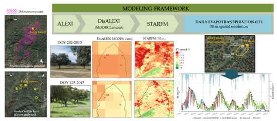
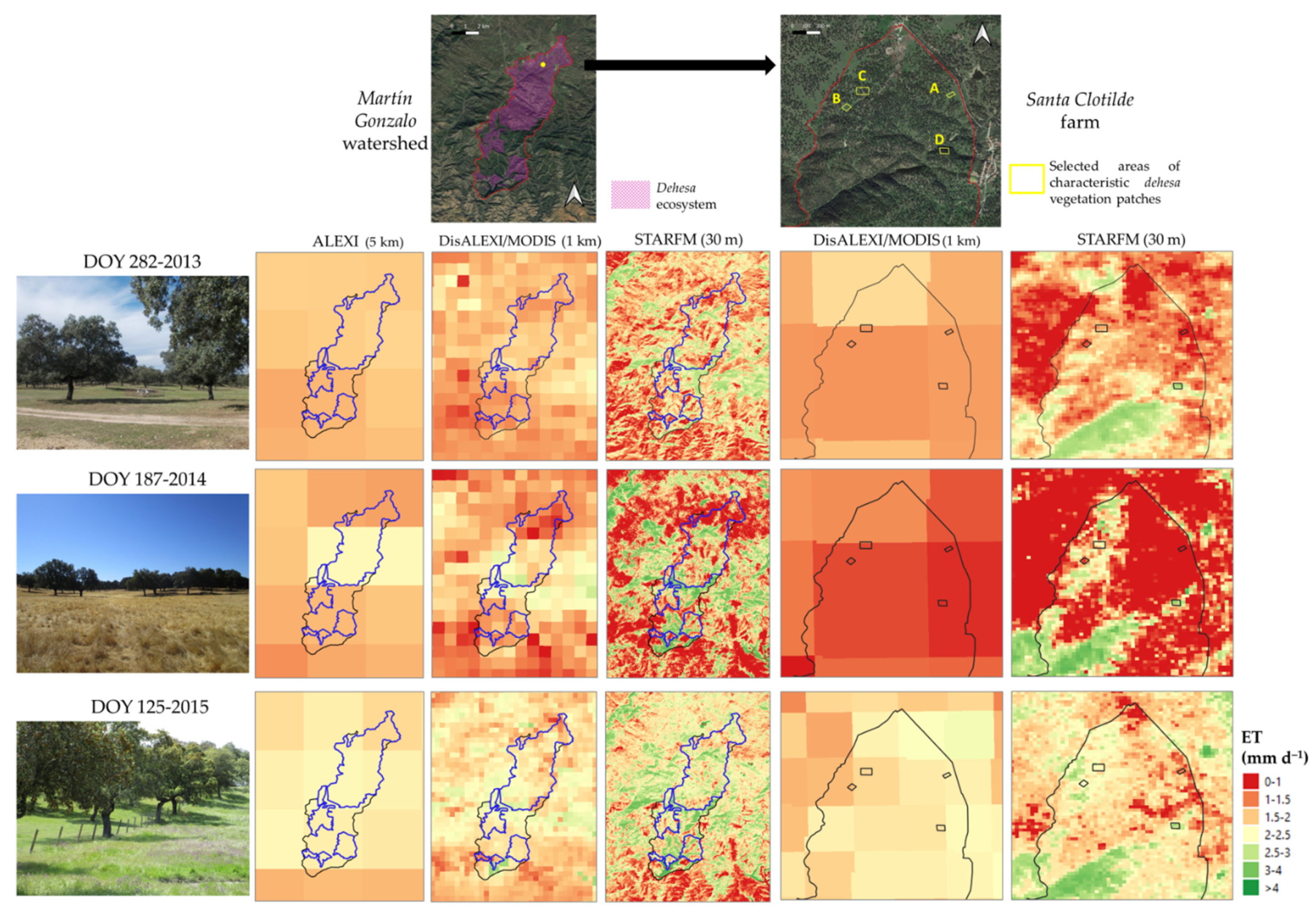
To evaluate the utility of a surface energy balance model (ALEXI/DisALEXI) and the STARFM data fusion technique, using multiple remote sensing platforms (Landsat 7/8 and MODIS), to estimate high-resolution ET in time and space over the complex canopy structure of Mediterranean oak savannas.
(ii)
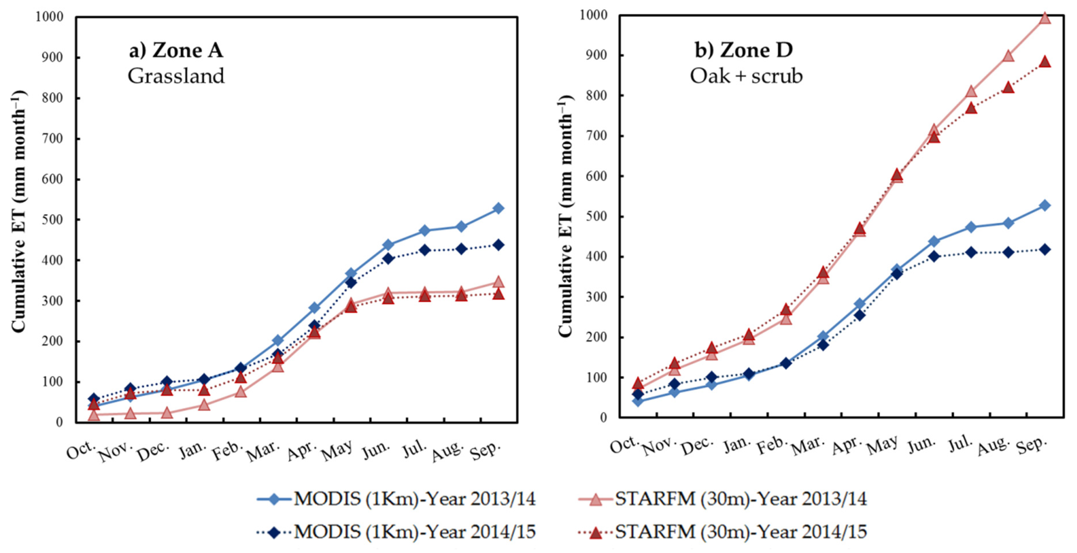
To analyze the opportunities offered by this high-resolution product to provide information that is useful to improve the water and vegetation management of this agroforestry system at a field scale. To do that, we evaluated the water use patterns of the herbaceous stratum and other small heterogeneous vegetation patches typical of the dehesa (e.g., scrubs, humid areas, creek shore), which shape the landscape structure and reflect the existence of different micro-ecosystems and climates. Finally, the cumulative monthly ET generated by the different approaches with different spatial resolutions (1 km and 30 m) was quantified over the same vegetation patches.

2. Materials and Methods

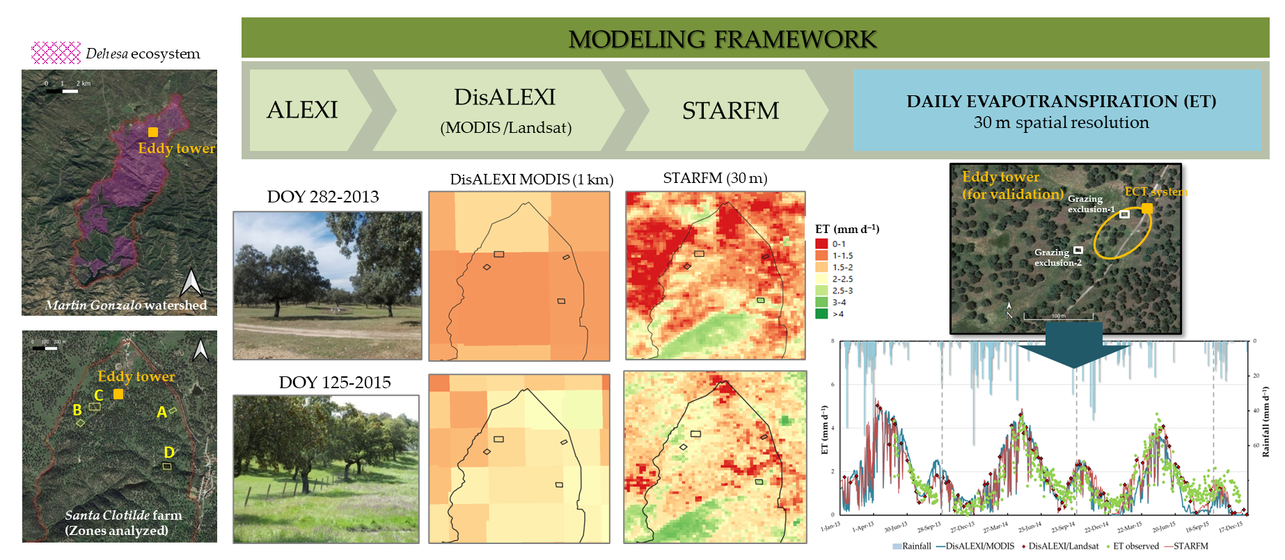
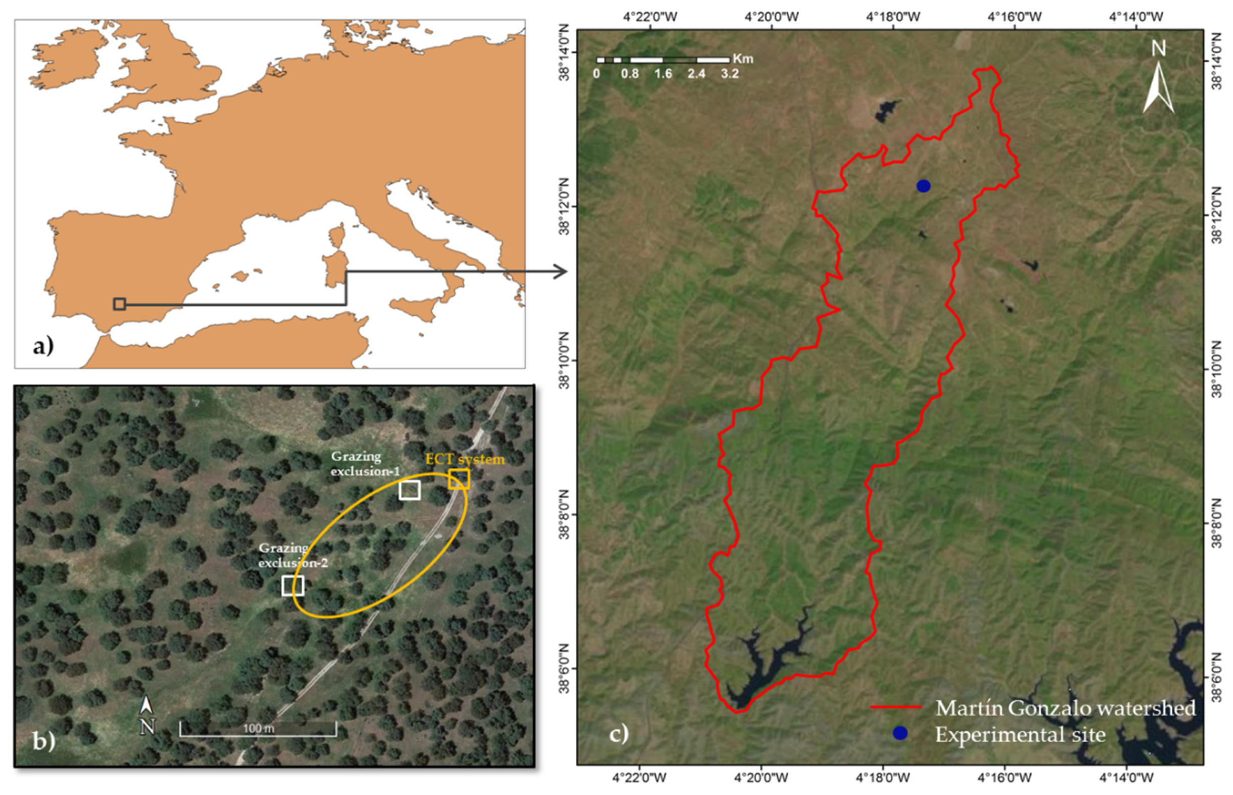
2.1. Description of the Study Area and Experimental Site

The study was conducted over the Martin Gonzalo watershed (48.4 km2), part of the larger Guadalquivir River basin located in Southern Spain (Figure 1a,c). The elevation range varies from 760 m in the north to 280 m at the outlet of the watershed, where there is a dam. The continental Mediterranean climate of this area is highly seasonal, with moderately cold winters alternating with hot and long dry summers. The rainfall presents intra- and inter-year variability, with an annual average of 895 mm (from 1990 to 2015) concentrated during spring and fall.
The landscape is mainly occupied by homogeneous dehesa, along with some conifer forests and olive groves. Dehesa is a Mediterranean oak savanna, whose canopy structure is composed of sparse clumped trees and a grassland or crops understory. In this ecosystem, extensive livestock production fed with acorns and grass is the main economic activity, but they also provide other uses, such as cork, cereal production, hunting, mushroom harvesting, and beekeeping. They offer as well multiple environmental services, such as biodiversity hotspots, water provisioning, CO2 fixation and high diversity of habitats [28,44].
Ground validation measurements were taken at an experimental site (Santa Clotilde, 38°12′ N, 4°17′ W, 736 m a.s.l, Figure 1c), located in a dehesa farm within the studied watershed. The setup included an eddy covariance tower (ECT) over the combined tree + grassland system and two grazing exclusion enclosures (over open grassland and under an oak tree respectively) to take into account the heterogeneity of the area (Figure 1b). All energy balance components: the turbulent fluxes of sensible heat (H) and latent heat (LE), net radiation (Rn) and the heat flux transport across the surface soil (G), were measured continuously.
The ECT system was installed on a tower at 18 m above ground level in April 2012, registering the ecosystem response as a whole (Figure 2a). The system included a 3D sonic anemometer (model CSAT3, Campbell Scientific Inc. Mention of trade names or commercial products in this publication is solely for the purpose of providing specific information and does not imply recommendation or endorsement by the U.S. Department of Agriculture) that measures horizontal and vertical fluctuations of temperature and wind speed, and a hygrometer (model KH20, Campbell Scientific Inc.) to estimate water vapor fluctuations, the latter being replaced in 2015 by an open Path CO2/H2O Gas Analyzer LICOR-7500, taking simultaneous measurements of carbon dioxide and water vapor in turbulent air structures (Figure 2b). These eddy covariance measurements were recorded with a frequency of 10 Hz and corrected for density effects due to heat and water vapor transfer [45].
A relative humidity and air temperature probe (model HMP155, Vaisala) and a net radiometer (model NR-Lite, Kipp&Zonen, Delft, Netherlands) to obtain the net radiation were also installed at the tower. In 2015, the net radiometer was replaced by a four-component-net-radiation sensor (model NR01, Hukseflux Thermal Sensors, Delft, Netherlands) (Figure 2b). More information on the experimental site and the equipment can be found in Andreu et al. [20] and Carpintero et al. [46].
The quality of the energy balance fluxes measured with the ECT was tested by Andreu et al. [20] for the 2012 summer season, resulting in an average closure balance (Rn − G = LE + H) of 86% of available energy. For the period 2014–2015, the closure balance was 91%. For the comparison with modeled LE, the latent heat fluxes obtained by forcing the closure of the energy balance with the residual method was preferred to direct LE measurement. This method assumes that the sensible heat, H, is correctly measured and LE is obtained by solving the surface energy balance equation. Daytime-integrated energy fluxes were calculated by averaging half-hourly values focusing on daytime fluxes and not considering overnight fluxes.

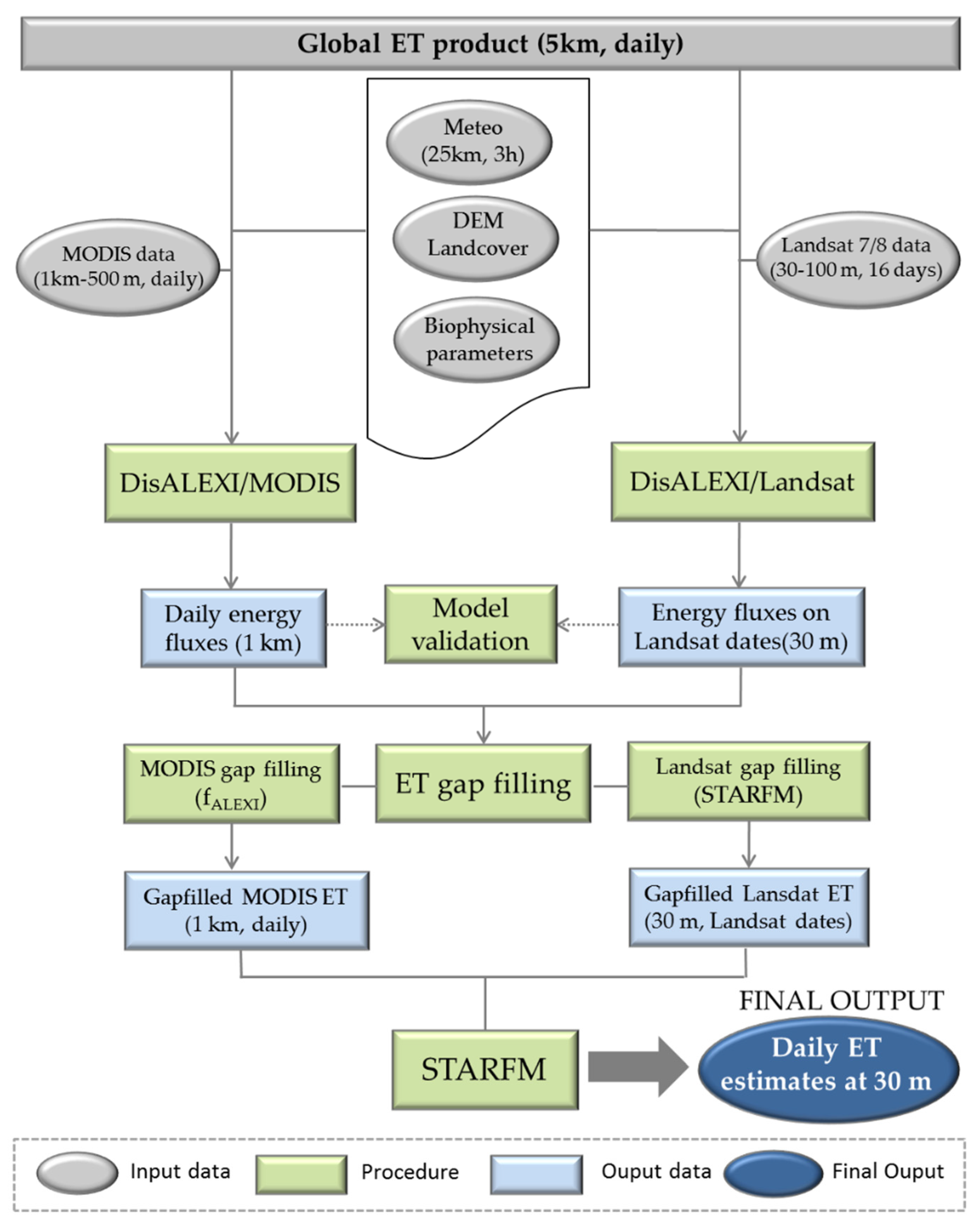
2.2. Modeling Framework

Figure 3 shows the flowchart of the modeling framework applied for the period 2013–2015. The process starts with a global ET product (5 km, daily) developed using the ALEXI model based on MODIS day-night temperature differences [47]. In the second step, the ALEXI ET fluxes are disaggregated to higher resolutions over the study area, using the flux disaggregation scheme DisALEXI applied to both MODIS (1 km, daily) and Landsat 7/8 (60–100 m, 16 days) images. Finally, both types of ET maps, the infrequent Landsat at 30 m resolution and the daily images at MODIS-scale generated by DisALEXI, are combined using the data fusion technique STARFM to provide ET estimates with both fine spatial (30 m) and temporal (daily) resolution.

2.2.1. ALEXI/DisALEXI Model

The Atmosphere-Land Exchange Inverse (ALEXI) model [24,25] and the associated flux disaggregation technique (DisALEXI) [26] are based on the Two Source Energy Balance (TSEB) model.
The TSEB model partitions the surface blackbody radiance into the soil/substrate (TS) and vegetated canopy (TC) blackbody temperatures, being weighted by the cover fraction of each component at the sensor view angle, f (φ), and resulting in:
T R A D ( φ ) ( f ( φ ) T c 4 + [ 1 f ( φ ) ] T s 4 ) 1 4
The surface energy balance is solved for the whole soil-canopy-atmosphere system, and for each individual component, with Equations (2) and (3):
R n s = H s + L E s + G
R n c = H c + L E c
where the subscripts “s” and “c” represent fluxes from the soil and canopy, respectively. Norman et al. [48] present a description of the original model, and further improvements can be found in Kustas et al. [18].
The ALEXI model was designed to reduce the use of ancillary meteorological data while maintaining a physically realistic representation of land-atmosphere exchange over a wide range of vegetation coverages. ALEXI implements the TSEB in a time-differential mode, applying this scheme two times during the morning, using surface radiometric temperature data generally provided by geostationary satellites. In this mode, the sensibility of the model to absolute temperature biases is reduced [25]. In ALEXI, TSEB is coupled with an atmospheric boundary layer model to internally simulate the effect of land-atmosphere feedback on the near-surface air temperature [49]. One limitation of this procedure is the dependence on geostationary datasets, with different calibrations and temporal extensions. For this reason, in this research, a global ET product developed using the non-geostationary MODIS sensor day-night temperature differences has been used. As a result, ALEXI generates surface energy fluxes at the continental scale, but at the coarse spatial resolution, of several km.
The DisALEXI scheme runs the TSEB using higher resolution thermal data from polar-orbiting satellites, such as MODIS or Landsat, for mapping finer spatial resolution fluxes. It iteratively adjusts the air temperature boundary conditions such that the disaggregated daily ET flux field reaggregates up to the coarse-resolution ALEXI regional baseline. This spatial disaggregation technique facilitates consistent flux evaluations at local to continental scales [49]. This ALEXI/DisALEXI framework has been widely evaluated across the United States and Europe [49,50,51].

2.2.2. Remote Sensing Data Fusion Method

The STARFM model [37] is a remotely sensed data fusion algorithm that allows an improvement of the temporal representation of ET variations between clear Landsat dates. It was originally designed to blend surface reflectance data, but the fusion of ET maps has been successfully conducted over a number of land covers by Cammalleri et al. [40,41] over rain-fed and irrigated agricultural areas in the Midwestern United States and over irrigated crops in Texas, by Semmens et al. [42] and Knipper et al. [17] over California vineyards, by Anderson et al. [16] over the California Delta and by Yang et al. [43,44,45,46,47,48,49,50,51,52] over forested landscapes. It combines information at a high-temporal frequency from MODIS and high-spatial-resolution from Landsat. STARFM compares one or two Landsat/MODIS image pairs acquired on the same day to predict maps at Landsat spatial scale on other MODIS dates.
Following the weighting function (Equation (4)), STARFM model predicts ET for the central pixel of a selected moving window at generic date (t0):
L ( x w 2 , y w 2 , t 0 ) = i = 1 w   j = 1 w   k = 1 n   W i j k [ M ( x i , y j , t 0 ) + L ( x i , y j , t k ) M ( x i , y j , t k ) ]
where w is the searching window size; (xw/2, yw/2) is the central pixel of this moving window; n is the number of Landsat and MODIS pairs used (in this case only one pair) and W is the weighting factor. The weighting function (W) integrates the spatial differences between the Landsat (L) and MODIS (M) images on the acquisition date tk and also the temporal differences between MODIS images from observed and predicted dates, tk and t0 respectively. The prediction for the central pixel only uses spectrally (or ET) similar pixels within the searching window. Further details about the STARFM model are provided by Gao et al. [37].

2.2.3. ET Data Gap Filling

Prior to the fusion algorithm, MODIS and Landsat ET maps produced by DisALEXI were preprocessed to fill the gaps created by clouds or instrument issues (e.g., the failure of scan-line corrector in Landsat-7 ETM+). The gaps in MODIS images were filled to obtain a full daily coverage at 1 km resolution. To accomplish this, the ratio between MODIS and ALEXI ET was computed on MODIS days (fALEXI = ET MODIS/ET ALEXI), then smoothed and filled using the Savitsky–Golay method described by Sun et al. [53]. The smoothed and filled fALEXI time series maps were then multiplied by daily ALEXI ET to obtain daily MODIS ET (Figure 3). The technique used to ensure optimal spatial coverage in Landsat maps employing the STARFM model was described by Yang et al. [43] (Figure 3). It combines the gapped ET image with a prediction from STARFM on the target date using a nearby MODIS-Landsat date pair.

2.2.4. Simple ET Interpolation Methods

In parallel to the application of the STARFM framework to obtain a daily 30 m ET series, daily ET values obtained with a simpler data interpolation method were also generated for comparison purposes. It used the potential ET and MODIS ET as scaling fluxes. The objective was to evaluate the advantages of using the STARFM technique with respect to these simpler and less demanding methods. In this interpolation approach, the ratio between the Landsat ET and a daily scaling flux (potential and MODIS ET) was computed on clear dates. These ratios (FPET = Landsat ET/Potential ET and FMOD = Landsat ET/MODIS ET) were then linearly interpolated in time and fused in the daily ET estimation.

2.3. Model Input Datasets

2.3.1. Landsat Data

This work employed a set of 82 Pre-collection and Collection 1 scenes (path 200/row 33) from the Landsat 7 and 8 satellites, acquired from January 2013 to December 2015. Scenes with high cloud coverage were excluded. The Landsat surface reflectance climate data record (SR CDR) (http://espa.cr.usgs.gov/, accessed on 2 September 2017) (distributed atmospherically corrected) was used to compute the leaf area index (LAI) and albedo parameters. A simple approach proposed by Liang et al. [54] was applied to calculate albedo at a 30 m resolution using six surface reflectance bands. To estimate LAI at 30 m on Landsat overpass dates, the regression tree approach developed by Gao et al. [55] was used, which was trained with samples from the MODIS LAI products and Landsat reflectance. This method has been successfully applied to annual and woody crops [42,55]. Landsat thermal band data were corrected for atmospheric and surface emissivity effects using the atmospheric radiative transfer model MODTRAN [56], and subsequently sharpened to the shortwave bands’ spatial resolution (30 m) using the Data Mining Sharpener (DMS) method [57].

2.3.2. MODIS Data

MODIS images from Collection 5 (at 1 km spatial resolution) and Collection 6 (500 m) with variable temporal resolution were also used as inputs in the DisALEXI application, including data of land surface temperature (LST; MOD11_L2), geolocation (MOD03), and LAI (MCD15A3). The radiometric temperature with a daily frequency was derived from the 5-min swath LST product, MOD11_L2. The 4-day LAI product, integrated into the TIMESAT algorithm [58], allowed for creating a smoothed and filled daily LAI time series.
As with other DisALEXI application inputs, the global albedo product from Boston University (ftp://rsftp.eeos.umb.edu/data02/Gapfilled/, accessed on 20 September 2017), in addition to the yearly and global MODIS product of land cover (MCD12Q1, 500 m) were included. The albedo data is a global gap-filled snow-free albedo product, which is temporally smoothed and composed over a global grid.

2.3.3. Meteorological Input Data and Vegetation Properties

The energy balance-based modeling framework requires several regional meteorological datasets: a series of surface atmospheric pressure, wind speed at 30 m, and air temperature and specific humidity at 2 m. These were provided every 3 h at a 25 km spatial resolution by the Climate Forecast System Reanalysis (CFSR) [59]. Hourly insolation data at a spatial resolution of 25 km were also obtained from the CFSR. As part of the regional information, a global digital elevation model at a 30 m resolution from ASTER (a product of METI and NASA) and the Andalusian land cover map 2010 were also employed.
A set of biophysical parameters associated with the vegetation in Mediterranean savanna ecosystems were used. The vegetation ground cover fraction, clumping factor and canopy height were calculated following Andreu et al. [20].

2.3.4. Input Data Filtering

In order to isolate errors caused by poor input data quality, the insolation and LST data were filtered for fluxes comparison using ground information. It is known that the quality of insolation data is the primary driver of the total energy available for the ET process [16], and TSEB is mostly driven by thermal information. Both variables were compared with the data measured at the experimental site, showing a mean relative error (mean absolute error/observed mean value; RE) of 9.4% in insolation and 14.5% in surface temperature. The days in which the RE value was higher than 25% in insolation data or higher than 50% in surface temperature were eliminated from the flux comparison analysis. Remotely sensed LST was compared with the half-hourly infrared temperature value corresponding to the time of the satellite overpass. In this case, given the variations between both values and the mismatch representativeness (IR thermometer is mostly measuring canopy—Figure 2b), the threshold considered for filtering the data is less restrictive than for radiation.

2.4. Global Remotely Sensed ET Product

The 8-day total ET provided by a product at a 500 m pixel resolution (MOD16A2, Collection 6) was used for comparison purposes. This data collection uses Mu et al.’s [60] improved algorithm. It is based on the logic of the Penman-Monteith equation which includes inputs of daily meteorological reanalysis data along with MODIS data, such as albedo, LAI, fraction of photosynthetically active radiation (FPAR) and land cover.

3. Results

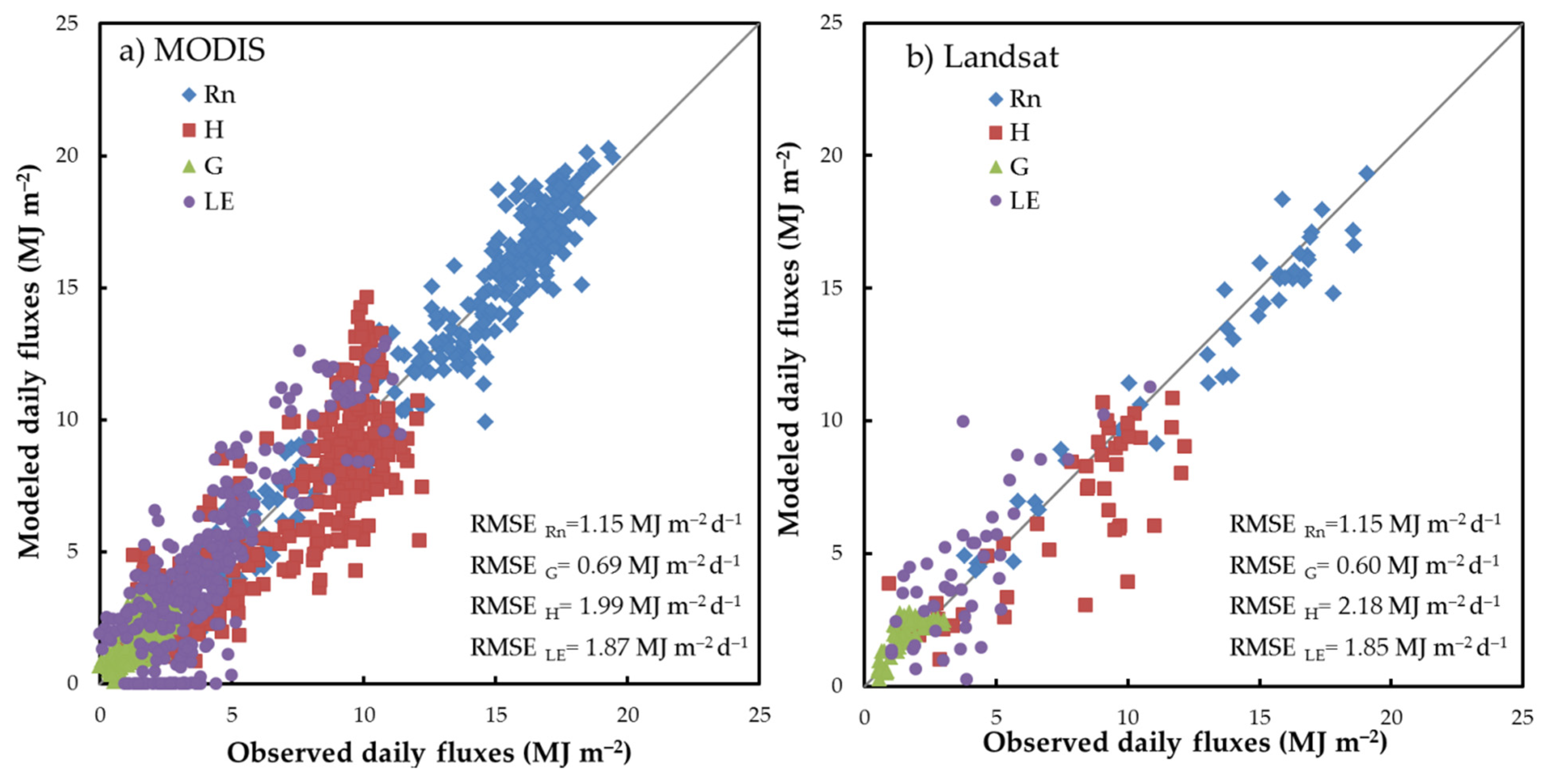
3.1. Evaluation of Surface Energy Fluxes at the Flux Tower Site

The frequency distribution of the wind direction at the ECT for 2015 showed the southwest as the predominant fetch. A footprint analysis was performed by estimating the contribution areas to daily fluxes for 132 days of 2015 as described by Hsieh et al. [61]. An extensive description of the methodology can be found in Kustas et al. [62]. Over the period analyzed, it is observed that 78% of the system ECT fluxes were collected from an area within 130 m upwind (Figure 1b), with the maximum contribution to the measured energy fluxes at approximately 33 m upwind. According to these results, average values of a 3 × 3 grid cell (with 30 × 30 m size-cell and located to the southwest of the ECT) of the modeled fluxes were evaluated.
The relationship between the daily energy fluxes (daytime integrated fluxes) observed at the ECT and modeled by the DisALEXI application is plotted in Figure 4, using MODIS (Figure 4a) and Landsat images (Figure 4b). The comparison was made on days in which both in-situ measurements and input information for the model were available, with a larger set of usable field data corresponding to 2014 and 2015. In addition, 22 days were filtered from the comparison with DisALEXI/MODIS and 5 days for DisALEXI/Landsat, due to the lack of input data quality (for further information about the input data filtering, see Section 2.3.4). A total of 313 days were used in the comparison for MODIS data and 44 images for Landsat. In all three years, there was a general shortage of clear images and/or field measurements during the last part of the winter and early spring. This is the rainy season for this region and the absence of available data hindered incorporating enough observations representative of this period in the statistical analysis. Statistical metrics, such as mean absolute error (MAE), root mean square error (RMSE), mean bias error (MBE) and coefficient of determination (R2) are presented for all the daily energy fluxes generated by DisALEXI application for the period 2013–2015 (Table 1).
Modeled Rn generally agreed with in-situ measurements (RMSE value of 1.15 MJ m−2 d−1 and R2 = 0.94–0.95). Rn behavior was different depending on the satellite sensor, slightly overestimated with MODIS data and underestimated when using Landsat images. Insolation (solar incoming radiation) inputs for both applications were the same, but with different albedo and fractional cover values to derive the energy available for the photosynthesis process. The soil heat flux estimations presented a good agreement (RMSE of 0.69 for MODIS and 0.60 MJ m−2 d−1 for Landsat), worthy of mention in this ecosystem with bare soil patches and high temperatures, where G can use up to 20% of the available energy.
RMSE and MAE errors observed with Landsat images were equal or slightly lower than those generated with MODIS for Rn, G and LE, possibly due to the better footprint representation of the higher resolution input data. The RMSE value for H was equal to 1.99 MJ m−2 d−1 when using MODIS data, and 2.18 MJ m−2 d−1 with Landsat. A general underestimation of the H flux can be observed in Figure 4, corroborated by the negative MBE values obtained with both sensors. Modeled LE fluxes had RMSE values of 1.87 MJ m−2 d−1 with MODIS, and 1.85 MJ m−2 d−1 with Landsat (in mass flux units, 0.76 mm d−1), with an overestimation of the modeled fluxes (MBE of 0.37 and 0.50 MJ m−2 d−1 or 0.15 and 0.20 mm d−1, respectively), except for low LE values. On the other hand, the values of the coefficient of determination were in the range 0.56–0.69 using Landsat and MODIS for both convective fluxes (H and LE).

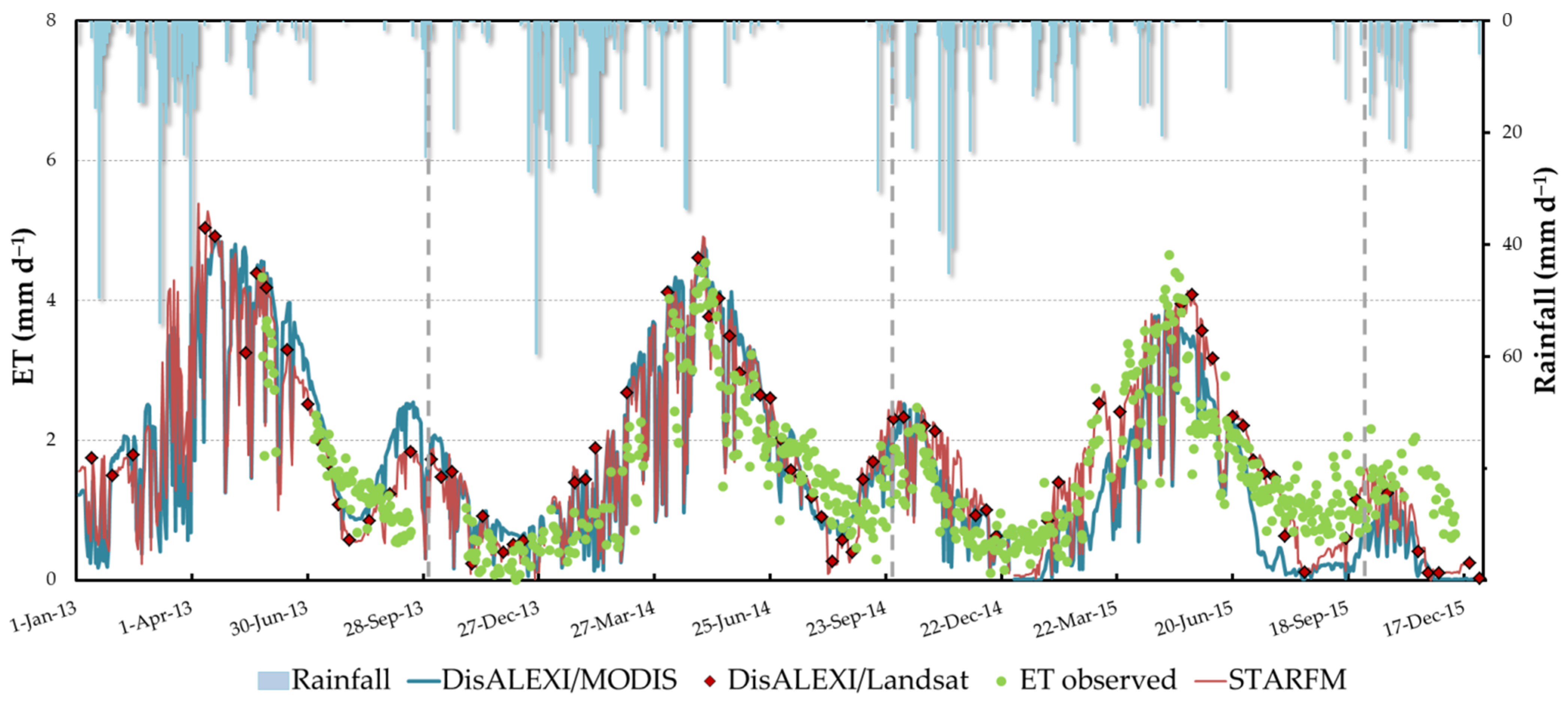
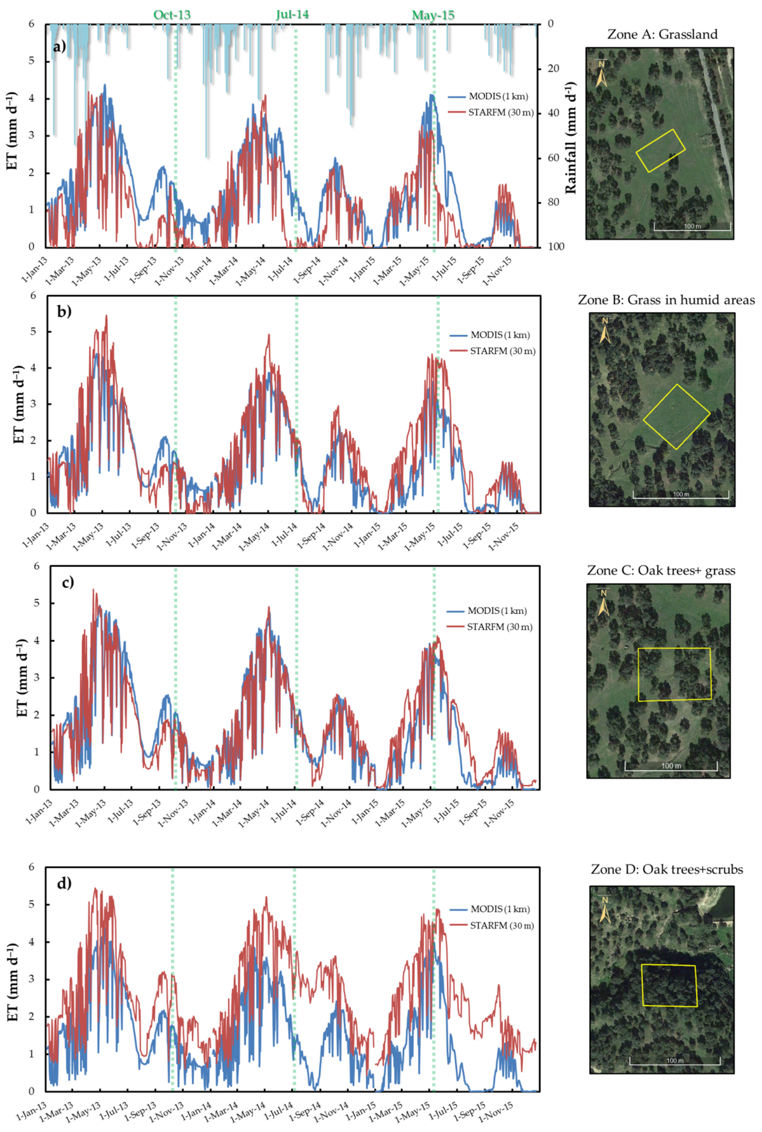
3.2. Analysis of ET Time Series from DisALEXI and STARFM

Figure 5 depicts the ET time series generated by DisALEXI (MODIS—1 km and Landsat—30 m) and STARFM approaches for the years 2013–2015, along with the closure-corrected ET measurements acquired by the dehesa ECT system and the rainfall observations. It can be observed in Figure 5 that in this ecosystem (with ~25% fraction tree cover) the annual ET curve is bimodal, with two distinct peaks of different sizes. The largest peak occurs during the spring, reaching maximum values of around 4–5 mm d−1. A second and smaller peak appears in autumn, with maximum values of around 2–2.5 mm d−1 in 2013–2014 and 1.5 mm d−1 in 2015. This pattern is closely linked to the distribution of the annual rainfall throughout the year, defining the general pattern of soil water availability, and the vegetation growth dynamics, as well as by the energy available for evaporation.
The modeled ET reasonably reproduced the temporal dynamics of consumptive water use observed by the flux tower instruments. In general terms, the maximum peaks reached in the spring seasons, as well as the gradual decrease of ET during the end of the spring and summer seasons (periods with higher data available) were accurately reproduced by the STARFM and DisALEXI approaches (Figure 5).
The annual ET modeled by STARFM was equal to 600 mm in the hydrological year 2013/2014 (1 October to 30 September), and 578 mm in the year 2014/2015, with rainfall values of 704 mm and 511 mm for each hydrological year, respectively. These results reflect the evolving vegetation water needs and how the ecosystem adapts to differing water availability conditions, with 193 mm less rainfall during the second year. It also highlights the major role that ET plays in the water balance of the system.
Looking at the details of seasonal water use more closely, we see that the water consumption in the spring of 2015 was similar to that of 2014, as well as the vegetation growth (NDVI values were similar for both years), even though the rainfall was considerably lower (spring rainfall of 120 mm in 2014 and 71 mm in 2015). In this case, the vegetation water consumption in the spring-2015 may have been tapping soil water storage from an unusually high rainfall in the previous autumn (311 mm in autumn—2014 compared to 103 mm of autumn—2013), pointing out the importance of the antecedent soil moisture conditions and the recharge of the subsurface layers.
During the summers, observed ET fell to low values (around 1.1 and 1.4 mm d−1 on average for the months of July and August), with minima around 0.7 mm d−1 at the end of the dry season (in early September before the first rainfalls). In addition to this summer-time soil-moisture limited minimum, a similar shut-down of the vegetation was observed during the winter (average ET around 0.7 in January and February), due to the lack of insolation.
Despite the generally good fit of ET estimations with ECT observations during the study period, some seasonal mismatches between modeled and observed fluxes can be identified. For example, modeled ET increased at the end of the summer in 2013 (on September 3) after a light rainfall event (<2 mm), while ET observations continued to decrease. While the second peak in the observed flux series is missing due to a gap in the field data from September 28, it appears that the rise in ET outlined by Landsat and STARFM preceded the observed rise following rainfall on September 27 (36 mm event). At the end of the dry season of 2014, similar behavior was observed with a gradual increase of modeled estimates starting on September 1, although it was not until September 17 when a significant rainfall event happened (approx. 46 mm). During the wet season in mid-May of 2015, the model showed a lagged response to a drydown that caused the vegetation to dry quickly. This may be related to smoothing/gap-filling in the baseline ALEXI time series, which can tend to smooth out abrupt changes in fPET.
A comparative analysis between the different daily ET series and the observed measurements at the ECT is shown in Table 2 including the quantitative performance of the following daily ET retrievals: (a) from DisALEXI 1 km gap-filled MODIS, (b) STARFM from Landsat-MODIS, and (c) from a simple Landsat-only interpolation technique (using the potential ET as a daily scaling input, through the ratio FPET). The analysis was carried out for a period of 584 days. Results obtained with the Landsat interpolated ET series using MODIS as a daily scaling input (not shown) are similar to those obtained using FPET.
The data fusion algorithm for estimating daily 30 m ET outperformed the simpler interpolation technique based on FPET and using MODIS 1-km ET, yielding an RMSE value of 0.67 mm d−1.

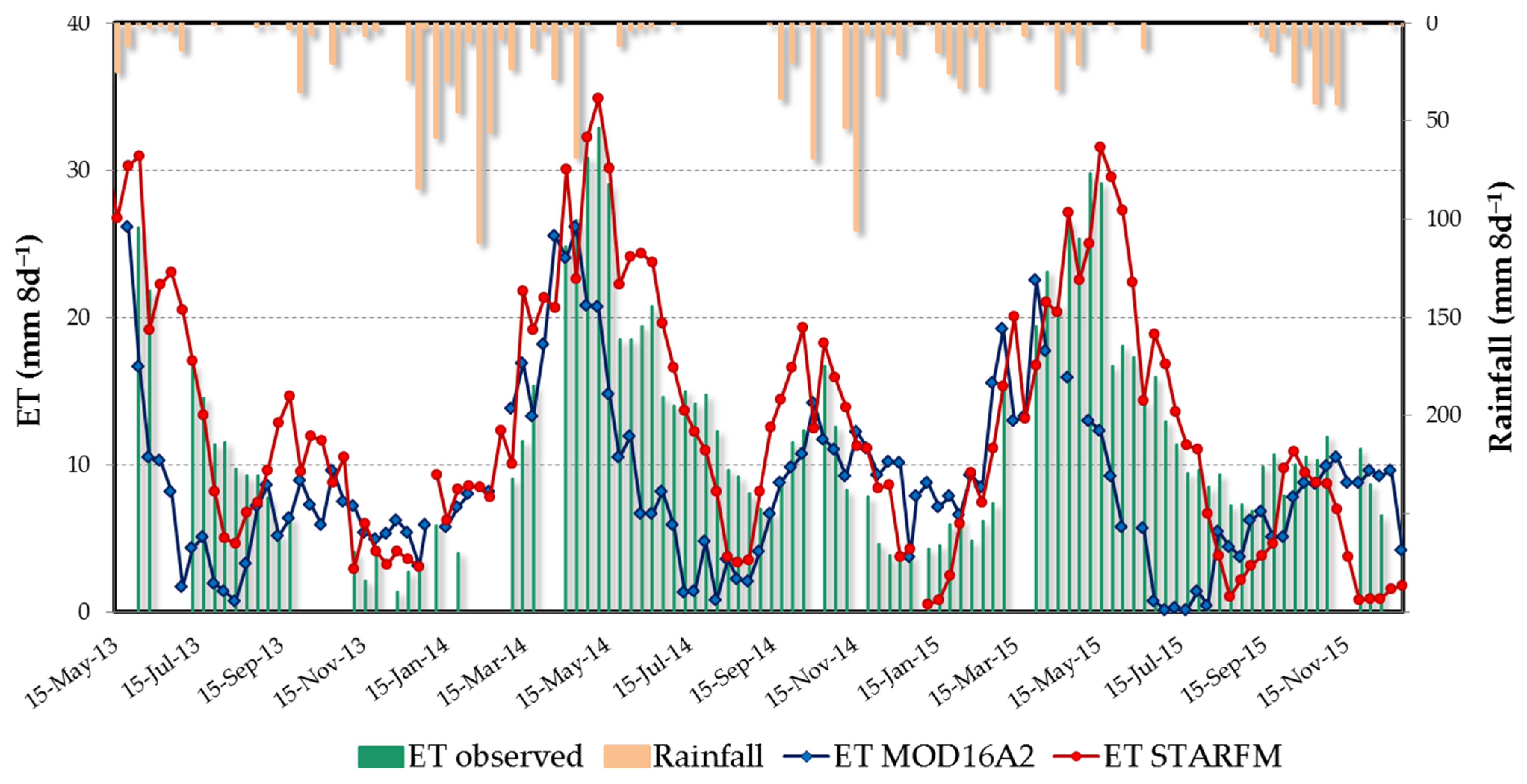
3.3. Evaluation of the MOD16A2 Global ET Product

Figure 6 shows data of the 8-day total ET layer provided by the global product MOD16A2 (500 m spatial resolution) at the tower pixel, together with the data observed at the ECT and the water consumption modeled by the STARFM approach. The MODIS ET product agreed poorly with the ECT observations (MAE = 0.79 mm d−1 and RMSE = 1.02 mm d−1), with a significant underestimation (MBE = −0.56 mm d−1). The error was unevenly distributed throughout the year, being more pronounced in the spring and summer seasons, and lessened in autumn and winter. This trend is observed in the three years and it highlights that the use of this product will underestimate ET rates over this semiarid ecosystem.

3.4. Water Resources Management at Field Scale Using High-Resolution ET Maps

At the field scale, the dehesa ecosystem presents variations in the distribution of vegetation strata (oak trees, grassland, crops, or scrubs) that affect the provisioning of ecosystem services and must be considered in the management of the livestock. Within this context, the evolution of daily ET at four characteristic micro-ecosystems/patches of the dehesa within the study area (Figure 1c), with different vegetation canopy structures and livestock feed production strategies has been analyzed at two spatial resolutions (30 m and 1 km) to evaluate the potential of Landsat-scale ET retrievals (Figure 7).
Zone A (1700 m2) is an open grassland without trees. It is a grazing area, which exhibits high temporal and spatial variability in vegetation growth. Zone B (2400 m2) is a pasture area where there is a land depression accumulating water through most of the year and maintaining high humidity conditions. Zone C (4300 m2) is a mixture of tree/grass, with an average tree fractional cover of around ~25%, common in dehesa production systems and similar to the ECT surrounding area. Acorn production to feed Iberian pigs is usually the main economic use of these landscapes. The final area, zone D (3300 m2), is located near a stream with a high ground fraction covered by trees and an evergreen underlayer of scrubs.
Significant differences were observed between the daily ET provided by DisALEXI/MODIS at a 1 km resolution and modeled ET with STARFM approach at a 30 m resolution, especially pronounced over zones A and D (Figure 7). Despite the relatively small area of these sites, the 30 m spatial resolution better captured the scale of heterogeneity in this landscape, whereas at 1 km, multiple vegetation covers are contributing, resulting in similar ET patterns for all the sites at this scale.
In the grassland area (Figure 7a), the STARFM 30 m ET decreases more rapidly in the spring than the MODIS-DisALEXI 1 km ET. This decrease corresponds to the drying of the herbaceous stratum, and thus the reduction in the available pasture for forage. Because there are no trees in the STARFM extraction area, transpiration flux is not appreciable during the summer months. The MODIS estimates include contributions from surrounding trees and therefore, maintain significant ET rates during the dry seasons. In each year, the pasture drying process started in May and ended in early to mid-July.
In contrast to zone A, in zone B the late spring decrease in ET is more gradual due to the high soil moisture conditions. The behavior during this season was accurately reproduced by the 30 m resolution model data. In this case, the 30 m and 1 km ET timeseries are more similar to the wet grassland (absent moisture limitations), mimics the transpiration curve of the surrounding trees. The main differences are during springtime peaks, where STARFM reaches values around 4.5–5 mm d−1, and about 4 mm d−1 with MODIS.
In zone C, the differences between DisALEXI/MODIS and STARFM were not pronounced due to the homogeneity of the surrounding landscape. This type of landscape is representative of the most common structure of the dehesa ecosystem, following a behavior similar to that described in Section 3.2.
Finally, in zone D we see that the 1 km MODIS information is not able to resolve the higher ET focused in this riparian forested area. ET estimates at 30 m suggest the use of groundwater (even shallow water from the creek) by the vegetation during summer, where the ET was maintained over 1.5 mm d−1, while MODIS ET incorporating surrounding grasslands drops to near 0. A more stable ET trend is seen over this river/scrub zone, where the ET reached similar maximums during the 3 years. These scrub species may have a high nutritional interest both for the domestic livestock, as well as for game species [63].
Cumulative annual water use curves, relevant for water resources management purposes, at 30 m and 1 km resolution are contrasted between relatively wet and dry hydrological years (2013/2014 and 2014/2015, respectively) over the zones A and D in Figure 8. These two areas were chosen because they showed higher scale-dependent differences (Figure 7). Total precipitation measured at the flux site was 704 mm in 2013/2014 and 511 mm in 2014/2015.
At both resolutions, cumulative ET is higher in the wet year (2013/2014) as expected. While cumulative ET at 1 km resolution was similar between zones (around 450–500 mm/year), the 30 m resolution data showed substantial variations between sites, with values ranging between 350 and 900 mm/year.
In the open grassland area, zone A (Figure 8a), the DisALEXI/MODIS approach produced an overestimation of the annual ET in the order of 120–180 mm when compared with the fusion model. Differences were more pronounced during the dry season when the STARFM curve remained stable from May on due to grass senescence. In zone D (Figure 8b), with transpiring vegetation throughout the year, the cumulative ET continuously increased at 30 m resolution. Neither intra- nor inter-annual significant variations in water consumption were observed with STARFM in this area close to a stream, probably due to higher use of groundwater by trees and scrubs and a lesser coupling of water consumption with rainfall events. MODIS cumulative ET showed a slight plateau during the months of July and August, capturing the behavior of the surrounding grassland area in the analysis. An underestimation of approximately 450 mm/year was quantified in this area using 1 km resolution data.
In addition, spatially distributed maps of ET over the Martin Gonzalo watershed and Santa Clotilde dehesa farm (Figure 1c) on three days, representative of different seasons of the period 2013–2015 are presented in Figure 9, highlighting the area with a dehesa ecosystem. They were produced by the ALEXI model (5 km), the DisALEXI/MODIS application (1 km) and the STARFM technique (30 m).
At the watershed scale, the more detailed representation of ET at a fine resolution provides a better understanding of the variability of the dehesa vegetation water consumption. At 30 m the variations in topography and soils, affecting the vegetation species composition and abundance, can be observed and are largely lost at the 1 km resolution and not existent at the 5 km scale. At the farm scale, the STARFM model allowed for the observation of ET variability in the different vegetation patches previously described, highlighting the existence of micro-ecosystems and climates at the local scale.

4. Discussion

4.1. DisALEXI Model Validation

The estimation of Rn flux presented an error (RMSE = 1.15 MJ m−2 d−1) slightly higher compared to other applications over agricultural areas [40,41,49], but it was aligned with the errors over sparse vegetation cover crops, such as grapevines [17,42] and forested/mosaic areas [16,43]. Ideally, future filtering of insolation inputs needs to be avoided in order to build an automated application, which should include a proxy to account for the quality of the input data. An alternative could be to migrate to an MSG Land-SAF satellite insolation product. Anderson et al. [64] tested different satellite insolation products generated by geostationary satellites, which significantly improved insolation performance over CFSR, although it did not translate into comparable improvement in the ET retrieval accuracy.
Likewise, the errors in H flux (RMSE value of 1.99 MJ m−2 d−1 when using MODIS data and 2.18 MJ m−2 d−1 with Landsat) were higher than other applications over agricultural areas (in the range of 1.2–1.7 MJ m−2 d−1 observed by Cammalleri et al. [40,41] and Semmens et al. [42]), but in the same range as those obtained in more complex vegetation [17,43].
In relation to LE flux modeled by DisALEXI, a similar behavior over another dehesa site (fluxnet code ES-LMA) using LST data measured in the field and MODIS images, was observed by Andreu et al. [20,21]. These authors used a lower Priestley-Taylor coefficient and stated that even integrating the green fraction and reducing the coefficient, during the dry season the flux was so low as to approach zero. Furthermore, the same trend had been previously observed by Carpintero et al. [65,66] in the study area, where the scheme was applied using a different meteorological dataset source and study period. In this regard, Burchard-Levine et al. [22] implemented the TSEB model over a dehesa area with modifications, considering phenological dynamics of this tree-grass ecosystem and assuming a dominant vegetation structure and cover for different seasons, and different seasonal vegetation parameters. This new adaptation improved the model performance, decreasing the overestimation of LE flux and RMSD errors compared to the application of TSEB assuming a single vegetation source.

4.2. Temporal Patterns in ET Curves

The ET time series estimated for the hydrological years 2013/2014 and 2014/2015 reflected the evolution of the vegetation water consumption, depending on water availability. Both hydrological years have similar ET rates, despite the lower precipitation rates in the second one. In 2014/15 water use exceeded the rainfall, suggesting that the vegetation tapped water from other sources to sustain transpiration rates within a threshold that plants could survive. It is known that oak tree roots are able to explore a large volume of soil, with a high dependence on deep water reserves [67,68]. Moreover, oaks form both arbuscular and ectotrophic mycorrhizae, and create mycorrhizal symbioses with partners, adapting to different conditions and accessing many different resources [69].
The similarity of water consumption in spring 2015 with respect to 2014 (with a significantly lower rainfall but an unusually high rainfall in the previous autumn) highlighted the importance of significant antecedent rainfall events to recharge the subsurface layers. In this sense, Fernández [70] found a significant correlation between grassland species abundance in the dehesa and autumn rainfall.
The ET values observed during the summers (Figure 5; minima values of 0.7 mm d−1 at the end of the dry season) were comparable with David et al.’s results [71], who found that oak trees maintained transpiration rates above 0.7 mm d−1 during the dry season with more than 70% of the transpired water being taken from groundwater sources. In seasons with low LE values (summers and winters), the uncertainty in the data observed by the eddy covariance system [72], added to the fact that LE flux was obtained by closing the balance with the residual method must be considered in the error assessment.
The accuracy of the different modeled daily ET series, shown in Table 2, is below the target error of 0.8 mm d−1 suggested by Seguin et al. [73]. The errors (RMSE = 0.67 mm d−1 with STARFM approach) were close to those found by other authors for woody sparse semiarid crops [21,74,75], and slightly higher than the RMSE value (~0.5 mm d−1) found by Campos et al. [76] and Carpintero et al. [46] in a dehesa ecosystem using a locally calibrated remote sensing-based soil water balance.

4.3. Performance of MOD16A2 ET

Sriwongsitanon et al. [77] showed a strong agreement of MOD16A2 values with the bulk ET computed using a water balance framework in the forested humid tropics of Thailand, on a monthly and annual scale. The estimations from that study were consistent with the soil moisture conditions and land use classes. An acceptable accuracy of this product was also found by Niyogi et al. [78] and Aguilar et al. [79] for water consumption monitoring over agricultural areas in Indiana (Midwestern United States) and Northwestern Mexico. Comparisons of this product with in-situ measurements at 15 flux tower sites with different climates and biome types ranging from croplands, grasslands, shrublands, savannas, to forests over Europe were evaluated by Hu et al. [80]. The global ET was consistent over most of Europe, with the best results over crops and meadows located in a temperate and humid climate. However, the seasonal performance of MOD16A2 was worse over vegetation under a semiarid climate, with RMSE equal to 1.17 mm d−1, comparable to the error found in this work (Figure 6; RMSE = 1.02 mm d−1). Global product ET was always underestimated for a dehesa ecosystem in Spain (similar study area and results to those of this work), demonstrating the weakness of this algorithm over limited water availability conditions [80]. The same behavior of ET underestimation was observed over a semiarid region in Iran [81], highlighting the high dependence of MOD16A2 performance with the climate type.
As shown in Figure 6, through the STARFM framework application we were capable of estimating with higher accuracy the temporal trend of ET (8 mm d−1) for this semiarid ecosystem, when compared with the MOD16A2 product.

4.4. Variability of Dehesa Vegetation Water Use at Field Scale

Dehesa landscape structure features, with variations in the distribution of vegetation strata, are associated with the creation of different microclimates, directly influencing ecological processes, such as plant regeneration and growth, soil respiration, nutrient cycling, and wildlife habitats [35].
The trends observed in the grassland area (zone A; Figure 7a), where the pasture drying process started in May and ended in early to mid-July, were consistent with the pasture production cycle observed in a similar dehesa farm in Spain (Las Majadas). The maximum production was obtained in the spring (around 60–70%) and autumn (15–20%), while the pasture growth was at a minimum in winter (5–15%) and zero in the summer [28]. Information about the pasture drying date at Landsat-scale, for which a high temporal frequency is crucial, can benefit the assessment of the nutritional quality for livestock feed [28]. The ET behavior in zone B (Figure 7b), where high humidity conditions existed, demonstrates the greater transpiration and production capacity of these moist grasslands, important for managing grazing rotations.
Due to the great expansion of the zone C vegetation structure (Figure 7c; a mixture of grass and trees with a low coverage fraction), previous applications of models for estimating water consumption at a low spatial resolution (from 1 km to 5 km) generally have worked well over this ecosystem. These models have provided very useful information at the basin or regional scale [20,21,23]. In zone D, the high spatial resolution ET reflects the presence of dense evergreen vegetation transpiring throughout the year. These areas provide essential ecosystem services, such as shelter for livestock and wildlife (rabbits, Iberian Lynx, etc.), or the creation of specific conditions under the canopy, with different radiation interception, and soils with increased fertility and water retention [82].
The spatial variability in the ET maps is represented in Figure 9 over the Martin Gonzalo watershed (left) and Santa Clotilde farm (right). From a hydrological modeling viewpoint, the 30 m resolution ET product may be very useful to identify and delineate hydrological zones with different water storage capacities and runoff processes within the basin. Nevertheless, the coarse resolution may be enough for regional managing purposes, such as drought monitoring. At the field scale, regular availability of this type of map can lead to developing better agricultural management decisions related to grazing rotations, delineating areas containing fragile ecosystems and important ecological riparian areas with higher water holding capacity and vegetation cover that can sustain a wide diversity of plant and animal species.

5. Conclusions

The ALEXI/DisALEXI model and the STARFM data fusion technique adequately estimated the ET dynamics of a Mediterranean oak savanna at fine spatial and temporal resolution (30 m, daily) for the period 2013–2015. The energy fluxes provided by DisALEXI using MODIS images (1 km, daily) and Landsat images (60–100 m, 16 days) were compared with in-situ measurements from an eddy covariance flux tower system. The modeled fluxes compared reasonably well to field observations, with RMSE values ranging between 0.60 and 2.18 MJ m−2 d−1 depending on the sensor resolution and the flux component, a similar range to those obtained by other authors over complex landscapes. In addition, the daily 30 m ET series from STARFM model obtained a RMSE value of 0.67 mm d−1, which is considered an acceptable error for dehesa management purposes.
The ET time series generated by both approaches, DisALEXI and STARFM with different resolutions, showed an annual bimodal behavior of the vegetation water consumption over the dehesa structure (grass and trees, with a tree cover fraction of 25%), with two marked peaks of different magnitudes (around 4–5 mm d−1 during the spring, and between 1.5 and 2.5 mm d−1 in the autumn). Modeled ET accurately reproduced the temporal dynamics of the water consumed by the vegetation, clearly linked to the distribution of the annual rainfall and the energy availability. Nevertheless, some difficulties of the model to reproduce certain abrupt changes in the ET behavior were identified, showing some limitations of the modeling scheme without more frequent observations and the importance of high-quality input data.
The results showed that when the data fusion model was applied, a slight improvement of RMSE, compared to using MODIS or simpler linear interpolations with Landsat data, was observed. This can be due to the combination of daily temporal frequency capturing the changes in ET and the high spatial resolution providing a better representation of the footprint of the flux tower. Modeled annual ET, close to 600 mm for both hydrological years despite their different rainfall regimes, provides an indicative value of current vegetation water needs and how the system adapts to meet these needs under the different water availability conditions. Holm oak’s ability to explore a large volume of soil and access groundwater resources under higher than typical water-limited conditions can explain a lack of a difference in ET between years and the minimum modeled values of transpiration of 0.7 mm d−1 at the end of the dry season. However, for periods of long-term and sustained drought, the ecosystem is likely to have a different response.
The major advantage of the data fusion technique and the high spatio-temporal resolution was found in the analysis of ET dynamics over different vegetation microbiomes, characteristics of the dehesa landscape. The results showed that high-resolution ET maps (daily, 30 m) can provide key information to better understand the hydrological functioning of different vegetation distributions difficult to detect at a 1 km pixel resolution and assist in decision making at the farm or local level. However, 1–5 km resolution ET information may suffice for regional monitoring and water planning purposes, such as regional drought detection and impacts on water resources of different biomes.

Author Contributions

Conceptualization, E.C., M.P.G.-D., M.C.A. and A.A; methodology, M.C.A., M.P.G.-D., E.C., A.A., C.H., F.G., W.P.K.; software and software application, M.C.A., C.H., F.G., E.C.; validation, E.C. and A.A.; data curation, E.C.; field data collection and processing, E.C. and A.A.; writing, review and editing, E.C., A.A., M.P.G.-D., M.C.A.; supervision, M.P.G.-D., M.C.A., W.P.K., F.G. All authors have read and agreed to the published version of the manuscript.

Funding

This research was funded by the FPU program—University Teachers Training—from the Department of Education, Culture and Sport. Dr. Andreu’s work was funded by the European Union’s Horizon 2020 Research and Innovation program under the Marie Skłodowska-Curie grant agreement No 703978. Additional support was provided by the project PP.PEI.IDF2019.004, co-funded at 80% by the European Regional Development Fund (ERDF), as part of the Andalusian operational program 2014–2020, and the project PID2019-107693RR-C22 (MCIU/AEI/FEDER, UE). This research was supported in part by the U.S. Department of Agriculture, Agricultural Research Service. USDA is an equal opportunity provider and employer.

Institutional Review Board Statement

Not applicable.

Informed Consent Statement

Not applicable.

Data Availability Statement

Data available contacting the principal researcher.

Acknowledgments

Theauthors would like to thank M. Ramos, J. Alfieri, J. Prueger and L. McKee for their help with field instrumentation installation as well as the maintenance, and measurements. We also would like to thank the collaboration of Santa Clotilde managers.

Conflicts of Interest

The authors declare no conflict of interest.

References

  1. Rodriguez-Iturbe, I.; Porporato, A.; Laio, F.; Ridolfi, L. Plants in water-controlled ecosystems: Active role in hydrologic processes and responce to water stress I. Scope and general outline. Adv. Water Resour. 2001, 24, 695–705. [Google Scholar] [CrossRef]
  2. Rundel, P.W.; Arroyo, M.T.K.; Cowling, R.M.; Keeley, J.E.; Lamont, B.B.; Vargas, P. Mediterranean Biomes: Evolution of Their Vegetation, Floras, and Climate. Annu. Rev. Ecol. Evol. Syst. 2016, 47, 383–407. [Google Scholar] [CrossRef]
  3. Gauquelin, T.; Michon, G.; Joffre, R.; Duponnois, R.; Génin, D.; Fady, B.; BouDagher-Kharrat, M.; Derridj, A.; Slimani, S.; Badri, W.; et al. Mediterranean forests, land use and climate change: A social-ecological perspective. Reg. Environ. Chang. 2018, 18, 623–636. [Google Scholar] [CrossRef]
  4. Cramer, W.; Guiot, J.; Marini, K. Climate and Environmental Change in the Mediterranean Basin–Current Situation and Risks for the Future; First Mediterranean Assessment Report; MedECC (Mediterranean Experts on Climate and Environmental Change); Union for the Mediterranean, Plan Bleu, UNEP/MAP: Marseille, France, 2020; ISBN 978-2-9577416-0-1. [Google Scholar]
  5. Milano, M.; Ruelland, D.; Fernandez, S.; Dezetter, A.; Fabre, J.; Servat, E.; Fritsch, J.M.; Ardoin-Bardin, S.; Thivet, G. Current state of Mediterranean water resources and future trends under climatic and anthropogenic changes. Hydrol. Sci. J. 2013, 58, 498–518. [Google Scholar] [CrossRef]
  6. Lionello, P.; Scarascia, L. The relation between climate change in the Mediterranean region and global warming. Reg. Environ. Chang. 2018, 18, 1481–1493. [Google Scholar] [CrossRef]
  7. Thiébault, S.; Moatti, J.; Ducrocq, V.; Gaume, E.; Dulac, F.; Hamonou, E.; Shin, Y.; Joel, G.; Boulet, G.; Guégan, J.; et al. The Mediterranean Region under Climate Change: A Scientific Update; IRD Éditions: Marseille, France, 2016; ISBN 978-2-7099-2219-7. [Google Scholar]
  8. Cramer, W.; Guiot, J.; Fader, M.; Garrabou, J.; Gattuso, J.P.; Iglesias, A.; Lange, M.A.; Lionello, P.; Llasat, M.C.; Paz, S.; et al. Climate change and interconnected risks to sustainable development in the Mediterranean. Nat. Clim. Chang. 2018, 8, 972–980. [Google Scholar] [CrossRef] [Green Version]
  9. García-Ruiz, J.M.; López-Moreno, I.I.; Vicente-Serrano, S.M.; Lasanta-Martínez, T.; Beguería, S. Mediterranean water resources in a global change scenario. Earth-Sci. Rev. 2011, 105, 121–139. [Google Scholar] [CrossRef] [Green Version]
  10. Turco, M.; Llasat, M.C.; von Hardenberg, J.; Provenzale, A. Climate change impacts on wildfires in a Mediterranean environment. Clim. Chang. 2014, 125, 369–380. [Google Scholar] [CrossRef]
  11. Bastiaanssen, W.G.; Menenti, M.; Feddes, R.A.; Holtslag, A.A.M. A remote sensing surface energy balance algorithm for land (SEBAL) 1 Formalation. J. Hydrol. 1998, 212–213, 198–212. [Google Scholar] [CrossRef]
  12. Cammalleri, C.; Agnese, C.; Ciraolo, G.; Minacapilli, M.; Provenzano, G.; Rallo, G. Actual evapotranspiration assessment by means of a coupled energy/hydrologic balance model: Validation over an olive grove by means of scintillometry and measurements of soil water contents. J. Hydrol. 2010, 392, 70–82. [Google Scholar] [CrossRef]
  13. Diak, G.R.; Whipple, M.S. Note on estimating surface sensible heat fluxes using surface temperatures measured from a geostationary satellite during FIFE 1989. J. Geophys. Res. 1995, 100. [Google Scholar] [CrossRef]
  14. Gonzalez-Dugo, M.P.; Neale, C.M.U.; Mateos, L.; Kustas, W.P.; Prueger, J.H.; Anderson, M.C.; Li, F. A comparison of operational remote sensing-based models for estimating crop evapotranspiration. Agric. For. Meteorol. 2009, 149, 1843–1853. [Google Scholar] [CrossRef]
  15. Timmermans, W.J.; Kustas, W.P.; Anderson, M.C.; French, A.N. An intercomparison of the Surface Energy Balance Algorithm for Land (SEBAL) and the Two-Source Energy Balance (TSEB) modeling schemes. Remote Sens. Environ. 2007, 108, 369–384. [Google Scholar] [CrossRef]
  16. Anderson, M.; Gao, F.; Knipper, K.; Hain, C.; Dulaney, W.; Baldocchi, D.; Eichelmann, E.; Hemes, K.; Yang, Y.; Medellin-Azuara, J.; et al. Field-scale assessment of land and water use change over the California delta using remote sensing. Remote Sens. 2018, 10, 889. [Google Scholar] [CrossRef] [Green Version]
  17. Knipper, K.R.; Kustas, W.P.; Anderson, M.C.; Alfieri, J.G.; Prueger, J.H.; Hain, C.R.; Gao, F.; Yang, Y.; McKee, L.G.; Nieto, H.; et al. Evapotranspiration estimates derived using thermal-based satellite remote sensing and data fusion for irrigation management in California vineyards. Irrig. Sci. 2019, 37, 431–449. [Google Scholar] [CrossRef]
  18. Kustas, W.P.; Norman, J.M. Evaluation of soil and vegetation heat flux predictions using a simple two-source model with radiometric temperatures for partial canopy cover. Agric. For. Meteorol. 1999, 94, 13–29. [Google Scholar] [CrossRef]
  19. Su, Z. The Surface Energy Balance System (SEBS) for estimation of turbulent heat fluxes. Hydrol. Earth Syst. Sci. 2002, 6, 85–100. [Google Scholar] [CrossRef]
  20. Andreu, A.; Kustas, W.P.; Polo, M.J.; Carrara, A.; González-Dugo, M.P. Modeling surface energy fluxes over a dehesa (oak savanna) ecosystem using a thermal based two-source energy balance model (TSEB) I. Remote Sens. 2018, 10, 567. [Google Scholar] [CrossRef] [Green Version]
  21. Andreu, A.; Kustas, W.P.; Polo, M.J.; Carrara, A.; González-Dugo, M.P. Modeling surface energy fluxes over a dehesa (oak savanna) ecosystem using a thermal based two source energy balance model (TSEB) II-Integration of remote sensing medium and low spatial resolution satellite images. Remote Sens. 2018, 10, 558. [Google Scholar] [CrossRef] [Green Version]
  22. Burchard-Levine, V.; Nieto, H.; Riaño, D.; Migliavacca, M.; El-Madany, T.S.; Perez-Priego, O.; Carrara, A.; Martín, M.P. Seasonal adaptation of the thermal-based two-source energy balance model for estimating evapotranspiration in a semiarid tree-grass ecosystem. Remote Sens. 2020, 12, 904. [Google Scholar] [CrossRef] [Green Version]
  23. González-Dugo, M.; Chen, X.; Andreu, A.; Carpintero, E.; Gómez-Giraldez, P.; Carrara, A.; Su, Z. Long-term water stress and drought monitoring of Mediterranean oak savanna vegetation using thermal remote sensing. Hydrol. Earth Syst. Sci. 2021, 25, 755–768. [Google Scholar] [CrossRef]
  24. Anderson, M.C.; Norman, J.M.; Diak, G.R.; Kustas, W.P.; Mecikalski, J.R. A two-source time-integrated model for estimating surface fluxes using thermal infrared remote sensing. Remote Sens. Environ. 1997, 60, 195–216. [Google Scholar] [CrossRef]
  25. Anderson, M.C.; Norman, J.M.; Mecikalski, J.R.; Otkin, J.A.; Kustas, W.P. A climatological study of evapotranspiration and moisture stress across the continental United States based on thermal remote sensing: 2. Surface moisture climatology. J. Geophys. Res. Atmos. 2007, 112, 1–13. [Google Scholar] [CrossRef]
  26. Norman, J.M.; Anderson, M.C.; Kustas, W.P.; French, A.N.; Mecikalski, J.; Torn, R.; Diak, G.R.; Schmugge, T.J.; Tanner, B.C.W. Remote sensing of surface energy fluxes at 101-m pixel resolutions. Water Resour. Res. 2003, 39. [Google Scholar] [CrossRef] [Green Version]
  27. Moreno, G.; Pulido, F.J. The Functioning, Management and Persistence of Dehesas. Agrofor. Eur. 2008, 10600, 127–160. [Google Scholar] [CrossRef]
  28. Moreno, G.; Cáceres, Y. System Report: Iberian Dehesas, Spain; AGFORWARD; Agroforestry for Europe: Plasencia, Spain, 2016. [Google Scholar]
  29. Díaz, M.; Tietje, W.D.; Barrett, R.H. Effects of Management on Biological Diversity and Endangered Species. In Mediterranean Oak Woodland Working Landscapes; Landscape Series, 2013; Campos, P., Huntsinger., L., Oviedo, J.L., Starrs, P.F., Díaz, M., Standiford, R.B., Montero, G., Eds.; Springer: Dordrecht, The Netherlands, 2013; Volume 16. [Google Scholar] [CrossRef]
  30. Plieninger, T.; Rolo, V.; Moreno, G. Large-scale patterns of Quercus ilex, Quercus suber, and Quercus pyrenaica regeneration in central-western Spain. Ecosystems 2010, 13, 644–660. [Google Scholar] [CrossRef]
  31. Coelho, C.; Ferreira, A.J.D.; Laouina, A.; Hamza, A.; Chaker, M.; Naafa, R.; Regaya, K.; Boulet, A.-K.; Keizer, J.J.; Carvalho, T.M.M. Changes in Land Use and Land Management Practices Affecting Land Degradation within Forest and Grazing Ecosystems in the Western Mediterranean. Sustain. Agrosylvopastoral Syst. Dehesas Montados 2004, 37, 137–153. [Google Scholar]
  32. Baldocchi, D.D.; Xu, L.; Kiang, N. How plant functional-type, weather, seasonal drought, and soil physical properties alter water and energy fluxes of an oak-grass savanna and an annual grassland. Agric. For. Meteorol. 2004, 123, 13–39. [Google Scholar] [CrossRef] [Green Version]
  33. Baldocchi, D.D.; Xu, L. What limits evaporation from Mediterranean oak woodlands—The supply of moisture in the soil, physiological control by plants or the demand by the atmosphere? Adv. Water Resour. 2007, 30, 2113–2122. [Google Scholar] [CrossRef]
  34. Joffre, R.; Rambal, S.; Damesin, C. Functional attributes in Mediterranean-type ecosystems. In Handbook of Functional Plant Ecology, 2nd ed.; Pugnaire, F.I., Valladares, F., Eds.; CRC Press Books: Boca Raton, FL, USA, 2008. [Google Scholar]
  35. Chen, J.; Saunders, S.C.; Crow, T.R.; Naiman, R.J.; Brosofske, K.D.; Mroz, G.D.; Brookshire, B.L.; Franklin, J.F. Microclimate in Forest Ecosystem the effects of different management regimes. Bioscience 1996, 49, 288–297. [Google Scholar] [CrossRef] [Green Version]
  36. Johnston, M.; Andreu, A.; Verfaillie, J.; Baldocchi, D.; Gonzalez-Dugo, M.P.; Moorcroft, P. Measuring surface temperatures in a woodland savanna: Opportunities and challenges of thermal imaging in an open-canopy ecosystem. Agric. For. Meteorol. 2021, 310, 108484. [Google Scholar] [CrossRef]
  37. Gao, F.; Masek, J.; Schwaller, M.; Hall, F. On the blending of the landsat and MODIS surface reflectance: Predicting daily landsat surface reflectance. IEEE Trans. Geosci. Remote Sens. 2006, 44, 2207–2218. [Google Scholar] [CrossRef]
  38. Walker, J.J.; De Beurs, K.M.; Wynne, R.H.; Gao, F. Evaluation of Landsat and MODIS data fusion products for analysis of dryland forest phenology. Remote Sens. Environ. 2012, 117, 381–393. [Google Scholar] [CrossRef]
  39. Zhu, X.; Chen, J.; Gao, F.; Chen, X.; Masek, J.G. An enhanced spatial and temporal adaptive reflectance fusion model for complex heterogeneous regions. Remote Sens. Environ. 2010, 114, 2610–2623. [Google Scholar] [CrossRef]
  40. Cammalleri, C.; Anderson, M.C.; Gao, F.; Hain, C.R.; Kustas, W.P. A data fusion approach for mapping daily evapotranspiration at field scale. Water Resour. Res. 2013, 49, 4672–4686. [Google Scholar] [CrossRef]
  41. Cammalleri, C.; Anderson, M.C.; Gao, F.; Hain, C.R.; Kustas, W.P. Mapping daily evapotranspiration at field scales over rainfed and irrigated agricultural areas using remote sensing data fusion. Agric. For. Meteorol. 2014, 186, 1–11. [Google Scholar] [CrossRef] [Green Version]
  42. Semmens, K.A.; Anderson, M.C.; Kustas, W.P.; Gao, F.; Alfieri, J.G.; McKee, L.; Prueger, J.H.; Hain, C.R.; Cammalleri, C.; Yang, Y.; et al. Monitoring daily evapotranspiration over two California vineyards using Landsat 8 in a multi-sensor data fusion approach. Remote Sens. Environ. 2016, 185, 155–170. [Google Scholar] [CrossRef] [Green Version]
  43. Yang, Y.; Anderson, M.C.; Gao, F.; Hain, C.R.; Semmens, K.A.; Kustas, W.P.; Noormets, A.; Wynne, R.H.; Thomas, V.A.; Sun, G. Daily Landsat-scale evapotranspiration estimation over a forested landscape in North Carolina, USA, using multi-satellite data fusion. Hydrol. Earth Syst. Sci. 2017, 21, 1017–1037. [Google Scholar] [CrossRef] [Green Version]
  44. Campos, P.; Huntsinger, L.; Oviedo, J.; Díaz, M.; Starrs, P.; Standiford, R.; Montero, G. Mediterranean Oak Woodland Working Landscapes: Dehesas of Spain and Ranchlands of California; Springer: Dordrecht, The Netherlands, 2013; ISBN 978-94-007-6706-5. [Google Scholar]
  45. Webb, E.K.; Pearman, G.I.; Leuning, R. Correction of flux measurements for density effects due to heat and water vapour transfer. Q. J. R. Meteorol. Soc. 1980, 106, 85–100. [Google Scholar] [CrossRef]
  46. Carpintero, E.; Andreu, A.; Gómez-Giráldez, P.J.; Blázquez, Á.; González-Dugo, M.P. Remote-sensing-basedwater balance for monitoring of evapotranspiration and water stress of a mediterranean Oak-Grass Savanna. Water 2020, 12, 1418. [Google Scholar] [CrossRef]
  47. Hain, C.R.; Anderson, M.C. Estimating morning changes in land surface temperature from MODIS day/night observations: Applications for surface energy balance modeling. Geophys. Res. Lett. 2017, 44, 9723–9733. [Google Scholar] [CrossRef]
  48. Norman, J.M.; Kustas, W.P.; Humes, K.S. Source approach for estimating soil and vegetation energy fluxes in observations of directional radiometric surface temperature. Agric. For. Meteorol. 1995, 77, 263–293. [Google Scholar] [CrossRef]
  49. Anderson, M.C.; Allen, R.G.; Morse, A.; Kustas, W.P. Use of Landsat thermal imagery in monitoring evapotranspiration and managing water resources. Remote Sens. Environ. 2012, 122, 50–65. [Google Scholar] [CrossRef]
  50. Anderson, M.C.; Kustas, W.P.; Norman, J.M.; Hain, C.R.; Mecikalski, J.R.; Schultz, L.; González-Dugo, M.P.; Cammalleri, C.; d’Urso, G.; Pimstein, A.; et al. Mapping daily evapotranspiration at field to global scales using geostationary and polar orbiting satellite imagery. Hydrol. Earth Syst. Sci. Discuss. 2010, 7, 5957–5990. [Google Scholar] [CrossRef] [Green Version]
  51. Anderson, M.C.; Norman, J.M.; Mecikalski, J.R.; Torn, R.D.; Kustas, W.P.; Basara, J.B. A multiscale remote sensing model for disaggregating regional fluxes to micrometeorological scales. J. Hydrometeorol. 2004, 5, 343–363. [Google Scholar] [CrossRef]
  52. Yang, Y.; Anderson, M.C.; Gao, F.; Wood, J.D.; Gu, L.; Hain, C. Studying drought-induced forest mortality using high spatiotemporal resolution evapotranspiration data from thermal satellite imaging. Remote. Sens. Environ. 2021, 265, 112640. [Google Scholar] [CrossRef]
  53. Sun, L.; Anderson, M.C.; Gao, F.; Hain, C.R.; Alfieri, J.G.; Sharifi, A.; McCarty, G.; Yang, Y. Investigating water use over the Choptank River Watershed using a multi-satellite data fusion approach. Water Resour. Res. 2017, 53, 5298–5319. [Google Scholar] [CrossRef] [Green Version]
  54. Liang, S. Narrowband to broadband conversions of land surface albedo: I. Algorithms. Remote Sens. Environ. 2000, 76, 213–238. [Google Scholar] [CrossRef]
  55. Gao, F.; Anderson, M.C.; Kustas, W.P.; Wang, Y. Simple method for retrieving leaf area index from Landsat using MODIS leaf area index products as reference. J. Appl. Remote. Sens. 2012, 6, 063554. [Google Scholar] [CrossRef]
  56. Berk, A.; Bernstein, L.S.; Robertson, D.C. MODTRAN: A Moderate Resolution Model for LOWTRAN 7; GL-TR-89-0122; Air Force Geophysics Lab: Bedford, MA, USA, 1987; p. 38. [Google Scholar]
  57. Gao, F.; Kustas, W.P.; Anderson, M.C. A data mining approach for sharpening thermal satellite imagery over land. Remote Sens. 2012, 4, 3287–3319. [Google Scholar] [CrossRef] [Green Version]
  58. Jönsson, P.; Eklundh, L. TIMESAT—A program for analyzing time-series of satellite sensor data. Comput. Geosci. 2004, 30, 833–845. [Google Scholar] [CrossRef] [Green Version]
  59. Saha, S.; Moorthi, S.; Pan, H.L.; Wu, X.; Wang, J.; Nadiga, S.; Tripp, P.; Kistler, R.; Woollen, J.; Behringer, D.; et al. The NCEP climate forecast system reanalysis. Bull. Am. Meteorol. Soc. 2010, 91, 1015–1057. [Google Scholar] [CrossRef]
  60. Mu, Q.; Zhao, M.; Running, S.W. Improvements to a MODIS global terrestrial evapotranspiration algorithm. Remote Sens. Environ. 2011, 115, 1781–1800. [Google Scholar] [CrossRef]
  61. Hsieh, C.I.; Katul, G.; Chi, T.W. An approximate analytical model for footprint estimation of scalar fluxes in thermally stratified atmospheric flows. Adv. Water Resour. 2000, 23, 765–772. [Google Scholar] [CrossRef]
  62. Kustas, W.P.; Alfieri, J.G.; Evett, S.; Agam, N. Quantifying variability in field-scale evapotranspiration measurements in an irrigated agricultural region under advection. Irrig. Sci. 2015, 33, 325–338. [Google Scholar] [CrossRef]
  63. Hajer, A.; López, S.; González, J.S.; Ranilla, M.J. Chemical composition and in vitro digestibility of some Spanish browse plant species. J. Sci. Food Agric. 2004, 84, 197–204. [Google Scholar]
  64. Anderson, M.; Diak, G.; Gao, F.; Knipper, K.; Hain, C.; Eichelmann, E.; Hemes, K.S.; Baldocchi, D.; Kustas, W.; Yang, Y. Impact of insolation data source on remote sensing retrievals of evapotranspiration over the California delta. Remote Sens. 2019, 11, 216. [Google Scholar] [CrossRef] [Green Version]
  65. Carpintero, E.; Semmens, K.; Anderson, M.C.; Andreu, A.; Gao, F.; Kustas, W.P.; González-Dugo, M.P. Use of remote sensing data fusion for daily evapotranspiration monitoring at watershed scale over a dehesa ecosystem. In Proceedings of the Fourth International Symposium on Recent Advances in Quantitative Remote Sensing, Valencia, Spain, 22–26 September 2014. [Google Scholar]
  66. Carpintero, E.; González-Dugo, M.P.; Hain, C.; Nieto, H.; Gao, F.; Andreu, A.; Kustas, W.P.; Anderson, M.C. Continuous evapotranspiration monitoring and water stress at watershed scale in a Mediterranean oak savanna. In Remote Sensing for Agriculture, Ecosystems, and Hydrology XVIII; SPIE: Bellingham, WA, USA, 2016; ISSN 0277-786X. ISBN 9781510604001. [Google Scholar]
  67. Cubera, E.; Morena, G. Effect of single Quercus ilex trees upon spatial and seasonal changes in soil water content in dehesas of central western Spain. Ann. For. Sci. 2007, 64, 355–364. [Google Scholar] [CrossRef] [Green Version]
  68. Moreno, G.; Obrador, J.J.; Cubera, E.; Dupraz, C. Fine root distribution in Dehesas of Central-Western Spain. Plant Soil. 2005, 277, 153–162. [Google Scholar] [CrossRef]
  69. Allen, M.F. How Oaks Respond to Water Limitation. In Proceedings of the Seventh California Oak Symposium: Managing Oak Woodlands in a Dynamic World; US Department of Agriculture, Forest Service, Pacific Southwest Research Station: Berkeley, CA, USA, 2015; pp. 13–21. [Google Scholar]
  70. Fernández-Alés, R. Response of Mediterranean grassland species to changing rainfall. A reply to Figueroa and Davy. Orsis 1993, 8, 121–126. [Google Scholar]
  71. David, T.S.; Henriques, M.O.; Kurz-Besson, C.; Nunes, J.; Valente, F.; Vaz, M.; Pereira, J.S.; Siegwolf, R.; Chaves, M.M.; Gazarini, L.C.; et al. Water-use strategies in two co-occurring Mediterranean evergreen oaks: Surviving the summer drought. Tree Physiol. 2007, 27, 793–803. [Google Scholar] [CrossRef] [PubMed] [Green Version]
  72. Burba, G.; Anderson, D. Eddy Covariance Flux Measurements. Ecol. Appl. 2010, 18, 211. [Google Scholar]
  73. Seguin, B.; Becker, F.; Phulpin, T.; Gu, X.F.; Guyot, G.; Kerr, Y.; King, C.; Lagouarde, J.P.; Ottlé, C.; Stoll, M.P.; et al. IRSUTE: A minisatellite project for land surface heat flux estimation from field to regional scale. Remote Sens. Environ. 1999, 68, 357–369. [Google Scholar] [CrossRef]
  74. Mateos, L.; González-Dugo, M.P.; Testi, L.; Villalobos, F.J. Monitoring evapotranspiration of irrigated crops using crop coefficients derived from time series of satellite images. I. Method validation. Agric. Water Manag. 2013, 125, 81–91. [Google Scholar] [CrossRef]
  75. Padilla, F.L.M.; González-Dugo, M.P.; Gavilán, P.; Domínguez, J. Integration of vegetation indices into a water balance model to estimate evapotranspiration of wheat and corn. Hydrol. Earth Syst. Sci. 2011, 15, 1213–1225. [Google Scholar] [CrossRef] [Green Version]
  76. Campos, I.; Villodre, J.; Carrara, A.; Calera, A. Remote sensing-based soil water balance to estimate Mediterranean holm oak savanna (dehesa) evapotranspiration under water stress conditions. J. Hydrol. 2013, 494, 1–9. [Google Scholar] [CrossRef]
  77. Sriwongsitanon, N.; Suwawong, T.; Thianpopirug, S.; Williams, J.; Jia, L.; Bastiaanssen, W. Validation of seven global remotely sensed ET products across Thailand using water balance measurements and land use classifications. J. Hydrol. Reg. Stud. 2020, 30, 100709. [Google Scholar] [CrossRef]
  78. Niyogi, D.; Jamshidi, S.; Smith, D.; Kellner, O. Evapotranspiration Climatology of Indiana, USA Using In Situ and Remotely Sensed Products. J. Appl. Meteorol. Climatol. 2020, 59, 2093–2111. [Google Scholar] [CrossRef]
  79. Aguilar, A.; Flores, H.; Crespo, G.; Marín, M.I.; Campos, I.; Calera, A. Performance Assessment of MOD16 in Evapotranspiration Evaluation in Northwestern Mexico. Water 2018, 10, 901. [Google Scholar] [CrossRef] [Green Version]
  80. Hu, G.; Jia, L.; Menenti, M. Comparison of MOD16 and LSA-SAF MSG evapotranspiration products over Europe for 2011. Remote Sens. Environ. 2015, 156, 510–526. [Google Scholar] [CrossRef]
  81. Jamshidi, S.; Zand-Parsa, S.; Pakparvar, M.; Niyogi, D. Evaluation of Evapotranspiration over a Semiarid Region Using Multiresolution Data Sources. J. Hydrometeorol. 2019, 20, 947–964. [Google Scholar] [CrossRef]
  82. Joffre, R.; Rambal, S. How tree cover influences the water balance of Mediterranean rangelands. Ecology 1993, 74, 570–582. [Google Scholar] [CrossRef]
Figure 1. (a,c) Location of the study area and experimental site; (b) Aerial photograph of validation site showing the distribution of the three fields discussed in the text. ECT: eddy covariance tower. The orange ellipse represents the predominant fetch of the ECT.
Remotesensing 13 03701 g001
Figure 2. (a) Eddy covariance tower (ECT) over the combined tree + grassland system; (b) equipment installed on the tower; (c) Grazing exclusion enclosure over open grassland.
Remotesensing 13 03701 g002
Figure 3. Flowchart of modeling framework applied to generate high resolution ET estimations.
Remotesensing 13 03701 g003
Figure 4. Comparison between observed and modeled daytime integrated energy fluxes obtained from DisALEXI procedure using (a) MODIS and (b) Landsat images for the years 2013–2015.
Remotesensing 13 03701 g004
Figure 5. ET time series over the dehesa ecosystem from DisALEXI/MODIS, DisALEXI/Landsat, STARFM approach and observed data with closure correction for 2013, 2014 and 2015. Blue bars illustrate rainfall events and gray vertical lines indicate the starting of a hydrological year.
Remotesensing 13 03701 g005
Figure 6. Comparison between observed, modeled by STARFM and MOD16A2 product ET for 2013–2015. Burnt orange bars illustrate rainfall events.
Remotesensing 13 03701 g006
Figure 7. Evolution of daily ET generated by DisALEXI/MODIS (1 km) and STARFM (30 m) over an area (denoted by the yellow polygons) of grassland (a), of grass in humid areas (b), of combined oak tree and grassland (c) and of oak trees and scrub (d). The green vertical dashed lines correspond to dates that are analyzed in Section 3.4.
Remotesensing 13 03701 g007
Figure 8. Evolution of cumulative monthly ET estimated by DisALEXI/MODIS and STARFM approaches for the hydrological year 2013/14 and 2014/15, over (a) zone A and (b) zone D.
Remotesensing 13 03701 g008
Figure 9. Distributed ET maps over the Martin Gonzalo watershed and Santa Clotilde dehesa farm derived from ALEXI (5 km), the DisALEXI/MODIS application (1 km) and the STARFM approach (30 m) on three representative dates of spring, summer, and autumn seasons. Blue lines show the dehesa ecosystem areas.
Remotesensing 13 03701 g009
Table 1. Statistical metrics of daily energy fluxes generated by DisALEXI application with MODIS and Landsat images for 2013–2015.
FluxŌ
(MJ m−2 d−1)
MAE
(MJ m−2 d−1)
RMSE
(MJ m−2 d−1)
MBE
(MJ m−2 d−1)
R2
MODISRn12.930.911.150.110.95
G1.590.560.690.350.52
H7.341.641.99−0.600.69
LE4.011.541.870.370.69
LandsatRn12.900.911.15−0.330.94
G1.520.460.600.320.60
H7.521.562.18−1.160.68
LE3.861.461.850.500.56
Ō = mean observed flux; MAE = mean absolute error; RMSE = root mean square error; MBE = mean bias error; R2 = coefficient of determination.
Table 2. Comparison of different daily ET retrievals modeled for the period 2013–2015.
MODISMODIS-Landsat (STARFM)Interpolated Landsat (Using FPET)
MAE (mm d−1)0.5890.5390.596
RMSE (mm d−1)0.7370.6730.749
MBE (mm d−1)0.0050.1030.158
Publisher’s Note: MDPI stays neutral with regard to jurisdictional claims in published maps and institutional affiliations.

