Article

Observations of Surface Currents and Tidal Variability Off of Northeastern Taiwan from Shore-Based High Frequency Radar

1
Institute of Ocean Technology and Marine Affairs, National Cheng Kung University, Tainan 701, Taiwan
2
Department of Oceanography, Naval Postgraduate School—NPS, Monterey, CA 93943, USA
3
Department of Marine Science, Naval Academy, Kaohsiung 813, Taiwan
*
Author to whom correspondence should be addressed.
Remote Sens. 2021, 13(17), 3438; https://doi.org/10.3390/rs13173438
Submission received: 6 June 2021 / Revised: 5 August 2021 / Accepted: 24 August 2021 / Published: 30 August 2021

Abstract

:
A network of high-frequency radars (HFRs) has been deployed around Taiwan. The wide-area data coverage is dedicated to revealing near real-time sea-surface current information. This paper investigates three primary objectives: (1) describing the seasonal current synoptic variability; (2) determining the influence of wind forcing; (3) describing the tidal current field pattern and variability. Sea surface currents derived from HFR data include both geostrophic components and wind-driven components. This study explored vector complex correlations between the HFR time series and wind, which was sufficient to identify high-frequency components, including an Ekman balance among the surface currents and wind. Regarding the characteristics of mesoscale events and the tidal field, a year-long high-resolution surface dataset was utilized to observe the current–eddy–tide interactions over four seasons. The harmonic analysis results derived from surface currents off of northeastern Taiwan during 2013 are presented. The results agree well with the tidal parameters estimated from tide-gauge station observations. The analysis shows that this region features a strong, mixed, mainly semidiurnal tide. Continued monitoring by a variety of sensors (e.g., satellite and HFR) would improve the understanding of the circulation in the region.

1. Introduction

Taiwan is situated between the Asian continent and the Pacific Ocean. It is a large island with a total coastline length of approximately 1200 km. In terms of atmospheric forcing, synoptic scale systems occur frequently in the spring, typhoons are common in summer, and frontal systems with strong winds and heavy rainfall are common in winter due to Taiwan’s subtropical climate. These variable monsoon systems drive sea-surface currents in the waters around the island. The interactions within the Western Boundary Current system between the warm Kuroshio Current and the rugged seafloor topography create a complex ocean current system around Taiwan [1,2]. The Kuroshio Current moves rapidly off of northeastern Taiwan and is commonly associated with seasonal cyclones worthy of long-term observations. To routinely monitor the currents and sea state around Taiwan, a current measurement network consisting of 19 SeaSonde® high-frequency radar (HFR) systems was established in 2008.
Remote measurement and monitoring of the sea state using HFRs has become an indispensable field in marine science and technology. Such systems have the capability to measure near real-time surface currents with good temporal resolution with operating frequencies ranging between 3 and 50 MHz. Regarding the general rule for electromagnetic radiation (EM) in the high-frequency band, the EM signal coupled with the sea surface can propagate via groundwaves over the horizon (OTH) [3]. In this study, two of the HFR network stations located off northeastern Taiwan were used as research instruments (the two green squares shown in Figure 1). HFRs have the capability to measure near real-time complete currents with good temporal and spatial resolutions. Figure 1 shows the area of maximum coverage in 2013. Areas with data coverage of 75% or more are shown in yellow, while areas with lower data coverage are shown in blue. The data coverage was calculated from the totals data (TUV) files, which are generated by combining the radial data from the two stations into the total velocities according to CODAR’s strict quality control (QA) mechanism. This study exploits the hourly TUV files from 2013 (8410 in total). Each circle in Figure 1 represents the position of a current vector. The data coverage over the course of the year, counted based on the number of observations, is displayed as a percentage. These radar coverage areas include the islands of Yonaguni and Iriomote, which are Japanese islands in the middle and on the eastern edge of the coverage area, respectively. The red triangles in Figure 1 represent tide (i.e., sea level elevation) stations on the shoreline. The data from these HFRs and tide stations are used in the subsequent analysis. In addition to routinely investigating mesoscale oceanic processes, the HFRs also provide the opportunity to resolve the tidal constituents around Taiwan. HFRs have been used to map tidal constituents and highlight the effects of tidal and wind drivers on diurnal movements [4]. While these direct observations of tidal-period current fluctuations exist for some regions, most tidal studies have been based on cross-validation of tide-gauge data and models [5]. This study utilizes both HFR and sea level observations to describe the tidal characteristics off northeastern Taiwan.
The main focus of this paper is to investigate the seasonal characteristics of the current patterns, the influence of wind forcing and the spatial distributions of tide constituents, taking advantage of the continuous time and space data from the coastal radar systems. There are some seasonal mesoscale events that appear in this area, but they have not been comprehensively studied. This paper is divided in five parts. In Section 2, this study describes the dataset and methods used. Selected data are compared with the HFR data depending on spatial and temporal availability, with Table 1 providing a summary of the datasets used and their temporal and spatial resolutions. The analysis methods used in this article to study the flow field, wind influence and tide are introduced in Section 3. Section 4 presents the results. To understand the dynamic processes in the area, this study describes the main features of this region and then compares the relationships between the HFRs and the surface geostrophic velocities (SGVs) and wind stress using complex correlation analyses. Then, harmonic analyses are used to describe the characteristics of the tides. Finally, Section 5 offers a discussion and conclusions.

2. Background

There are existing, regional research results on the seasonal variations of the surface currents [6,7]. To characterize the regional marine environment in terms of ocean circulation, this study organized the available remote sensing data for comparison and analysis. We use the surface currents off of northeastern Taiwan derived from the HFRs. These observations are compared against two other datasets. First, the surface currents are correlated with the surface geostrophic currents obtained from satellite altimeter observations and extracted from the Archiving Validation and Interpretation of Satellite Oceanographic (AVISO+) database. Next, the surface currents are correlated against the wind field data from the source known as the Cross-Calibrated Multi-Platform (CCMP) database. To characterize the regional tidal fluctuations, the tidal currents and tide types analyzed and derived from the HFRs are compared with the tidal constituents derived from sea level measurements from the coastline tide-gauge stations. All of the data used in this study are summarized in Table 1. In the following analysis of complex correlation of veering, this research is based on the shortest time resolution, i.e., daily, that Aviso+ can provide (as shown in Table 1, the temporal resolutions of the datasets are as follows: HFR is hourly, SGV is daily, and wind is 6 h). Therefore, this study performs a long-term averaging of hourly HFR data and 6-hourly wind data and then analyzes the complex correlation of veering with these three remote sensing datasets to analyze the influence of wind.

2.1. Remote Sensing Data

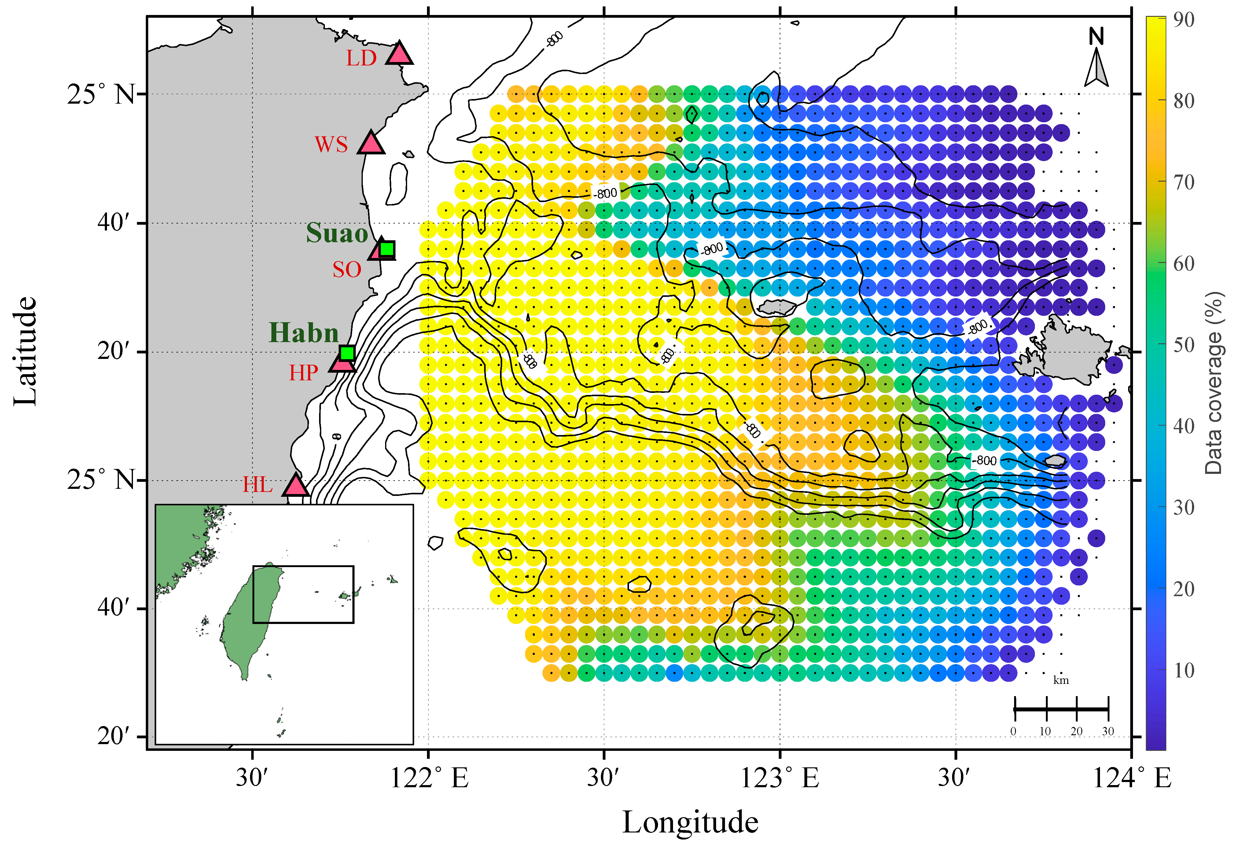
2.1.1. High-Frequency Radar

This study used HFR data from two long-range SeaSonde systems located at the Suao and Habn stations on the eastern coast of Taiwan, as shown in Figure 1. The northeastern region of Taiwan, as well as the Yonaguni and Iriomote Islands of Japan, are all within the maximum radar coverage of 292 km. The long-range SeaSonde systems were operated with a chirp signal centered at 4.4 kHz with an 18.38 kHz sweep bandwidth and a sweep repetition time of 1 s (as shown in Table 2). There is good correlation between the mean radial velocities measured by these two stations and the 20 m water-depth current data from the shipboard acoustic Doppler current profilers (SADCPs). It was also confirmed that there were no significant systematic deviations among these stations [8,9].

2.1.2. Aviso+

AVISO+ provides sea surface height (SSH) and SGV data in Mercator projection coordinates with a latitude range of 82° N to 82° S and a nominal cell size of 1/8°. To maximize the accuracy of the spatial and temporal resolutions, this dataset merged observations from multiple satellites, including Topex/Poseidon, Jason-1, Jason-2, GFO, ERS-1, ERS-2, and EnviSat. The SGV used in this study was one of the gridded products from satellite altimetry data; other products also included wind speed modulus and significant wave height [10]. Altimeter-derived surface geostrophic velocities have been used to explore variations in the Kuroshio Current east of Taiwan over time periods from a few weeks to several years. Hsin et al., (2013) [11] verified that the altimeter-based velocities are comparable to shipboard ADCP velocity composites, including the turning position, magnitude and pathway of the Kuroshio Current. Figure 2 shows the annual mean SGV around Taiwan in our study period. A significant meandering current with a high speed of approximately 70 cm/s was observed flowing northward along the eastern coast of Taiwan. The Kuroshio Current has been ascribed to the seasonal reversal of monsoonal winds via Ekman dynamics [12]. Sea surface currents derived by HFR contain wind, a mixture of geostrophic and ageostrophic constituents [13]. The satellite-derived current estimates, on the other hand, are limited to the geostrophic constituent by the physics of the measurement. Our approach, therefore, is to attempt to remove the geostrophic constituent from the HFR observations by subtracting the satellite-derived current estimates to form the residual currents. To understand the influence of wind forcing on HFR data, this study explored vector complex correlations between the HFR and satellite-derived SGV data and wind data to demonstrate high-frequency components in the following section.

2.1.3. CCMP Ocean Surface Wind Components

The CCMP derives wind retrievals from a number of satellite-borne passive and active microwave instruments. The dataset primarily combines instrument observations and cross-calibrated satellite microwave wind using variational analysis methodology (VAM) to produce 1/4° high-resolution gridded analyses. This data source provides gap-free ocean surface wind data with high temporal and spatial resolutions, which are useful for the study of large-scale air–sea interactions affecting the atmosphere and ocean. Winds are dynamic and constantly evolve over short periods of time. Accordingly, the CCMP provides 6 h vector wind data at 10 m above the sea surface, which is useful for subsequent correlation studies of HFR and SGV data [14].

3. Methodology

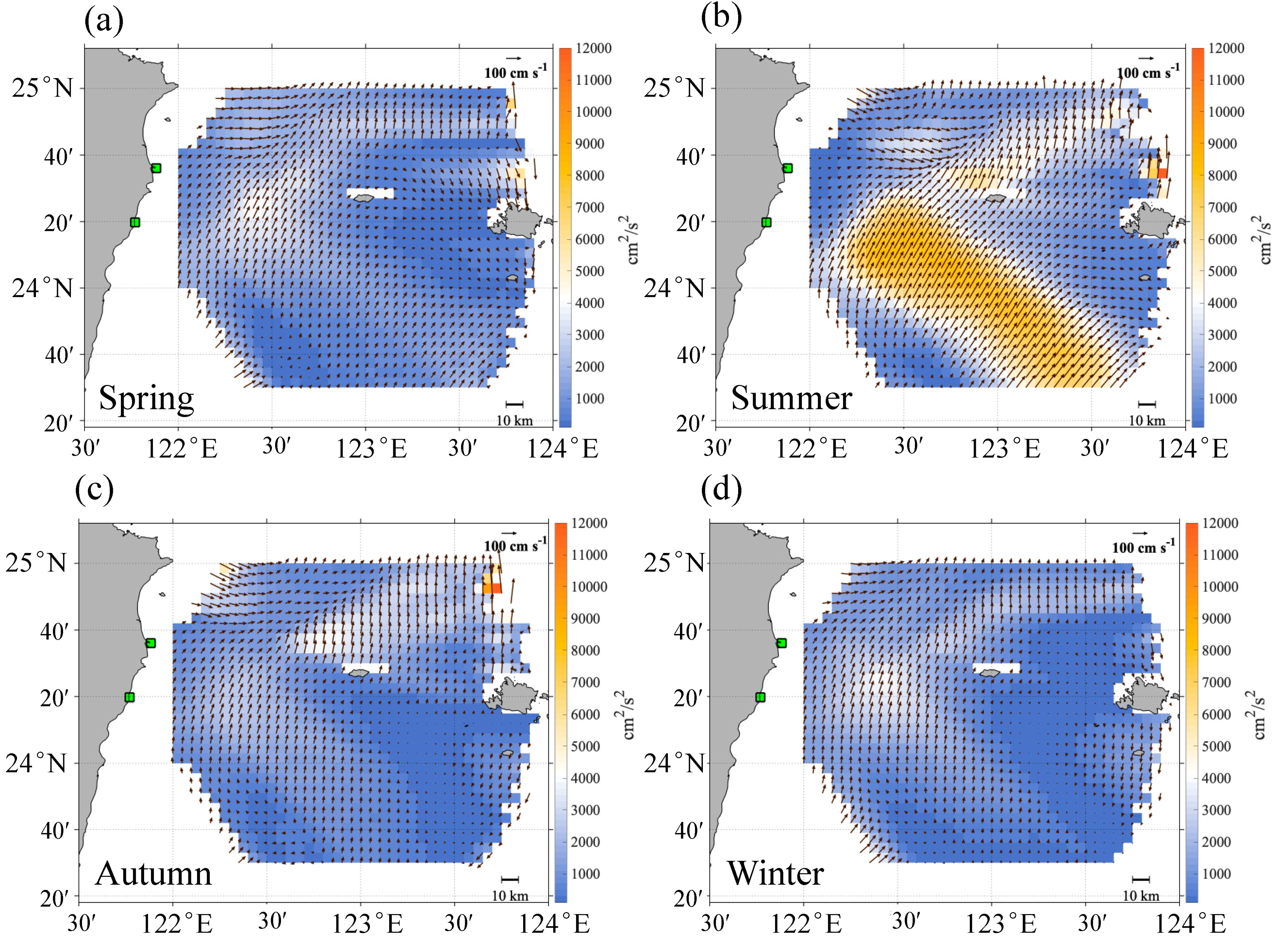
3.1. Eddy Kinetic Energy Distribution

To investigate the time-varying component of the current, the distribution of mean and eddy energy was given by the velocity values, which grouped in time and area boxes [15]. Eddy kinetic energy (EKE) values are time and space averages and commonly used to analyze the velocity field. For this purpose, it is necessary to average the currents in few representative boxes and display the time evolution of these spatially averaged currents [16]. However, this definition contains all processes that vary in time, including coherent mesoscale eddies, jets, waves, and large-scale motions. The EKE value per unit mass were given by
EKE = 1 2 × ( u 2 ¯ + v 2 ¯ )
where the mean velocity u ¯ , v ¯ in the horizontal and vertical directions and the departures u , v were calculated for each box.

3.2. Complex Correlation of Veering

Ocean currents can be depicted as a blend of geostrophic and ageostrophic terms, with the latter representing wind-driven ageostrophic currents [17]. HFRs have been utilized to derive wind-driven surface currents in many studies and to illustrate the connection between coastal currents and wind. Coastal currents respond rapidly to wind effects, with currents changing speed or reversing in response to changing wind patterns and wind stresses [17,18,19,20]. Since the angle between two observed vectors (e.g., currents and wind) can be a function of time, one method to investigate correlations is to find the average angular displacement between two vectors. The average deviation between a pair of two-dimensional time series can be obtained from the phase angle of the complex correlation coefficient [21]. Thus, the correlation between the radar-derived surface current measurements, SGV, and overwater winds can be analyzed by the complex correlation of veering. In this case, the vectors are represented as complex variables such that
w ( t ) = u ( t ) + i v ( t )
where w is a complex representation of the velocity time series at time t. To estimate the mean veering by weights, the averaging process is in accordance with the magnitude of the instantaneous vectors and is given by
α a v = t a n 1 < u 1 v 2 v 1 u 2 > < u 1 u 2 v 1 v 2 >
where the phase angle of average veering is expressed as αav and the complex correlation coefficient between two vector series is defined as their normalized inner product as u1, v1 and u2, v2. The results using the complex correlation technique are presented in the next section.

3.3. Harmonic Analysis

The tide is a phenomenon of periodic change in the sea water level, which heavily influences human activities at sea. Harmonic analysis is a time series analysis technique that can be applied to separate tidal components from other fluctuations at each observation grid location. Tidal patterns have been revealed using HFR observations [4,22,23]. Harmonic analysis is the process of calculating the amplitude and phase of the fundamental and higher-order harmonics of a periodic waveform and is sensitive to systematic signal changes [24].
The harmonic analysis in this study employed the T_Tide toolbox [25] to investigate and quantify tidally driven currents and thus explore coastal hydrodynamics. The procedure is dedicated to analysis phenomena of a periodically recurrent issue by the technique of breaking complicated mathematical curves into sums of comparatively simple components [26]. The technique was applied to locations on the HFR grid with more (75%) data coverage availability during the study period (Figure 1). There are 45 astronomical and 101 shallow-water constituents that can be chosen from a list, with all constituents arranged in a predefined order. The program ranks the tidal constituents based on their equilibrium amplitude.
Least-squares fitting can be used to determine the relative phase and amplitude of each frequency in the response [25]. The T_Tide toolbox can be corrected for the nodal modulation for each constituent k, which is converted into standard parameters to describe the tidal ellipse as follows:
L k = | a k | + | a k |
l k = | a k | + | a k |
θ k = a n g ( a k ) + a n g ( a k ) 2 m o d 180
g k = v k a n g ( a k ) + θ k
where ak and ak are a pair of complex values and Lk and lk are the lengths of the semimajor and semiminor axes of the ellipse, respectively. In addition, the inclination of the counterclockwise northern semimajor axis depends on east θk and Greenwich phase gk. These elliptical parameters are sufficient to further analyze the tidal elliptical properties of the specific field. The results using the T_Tide toolbox are presented in the next section.

4. Experimental Results

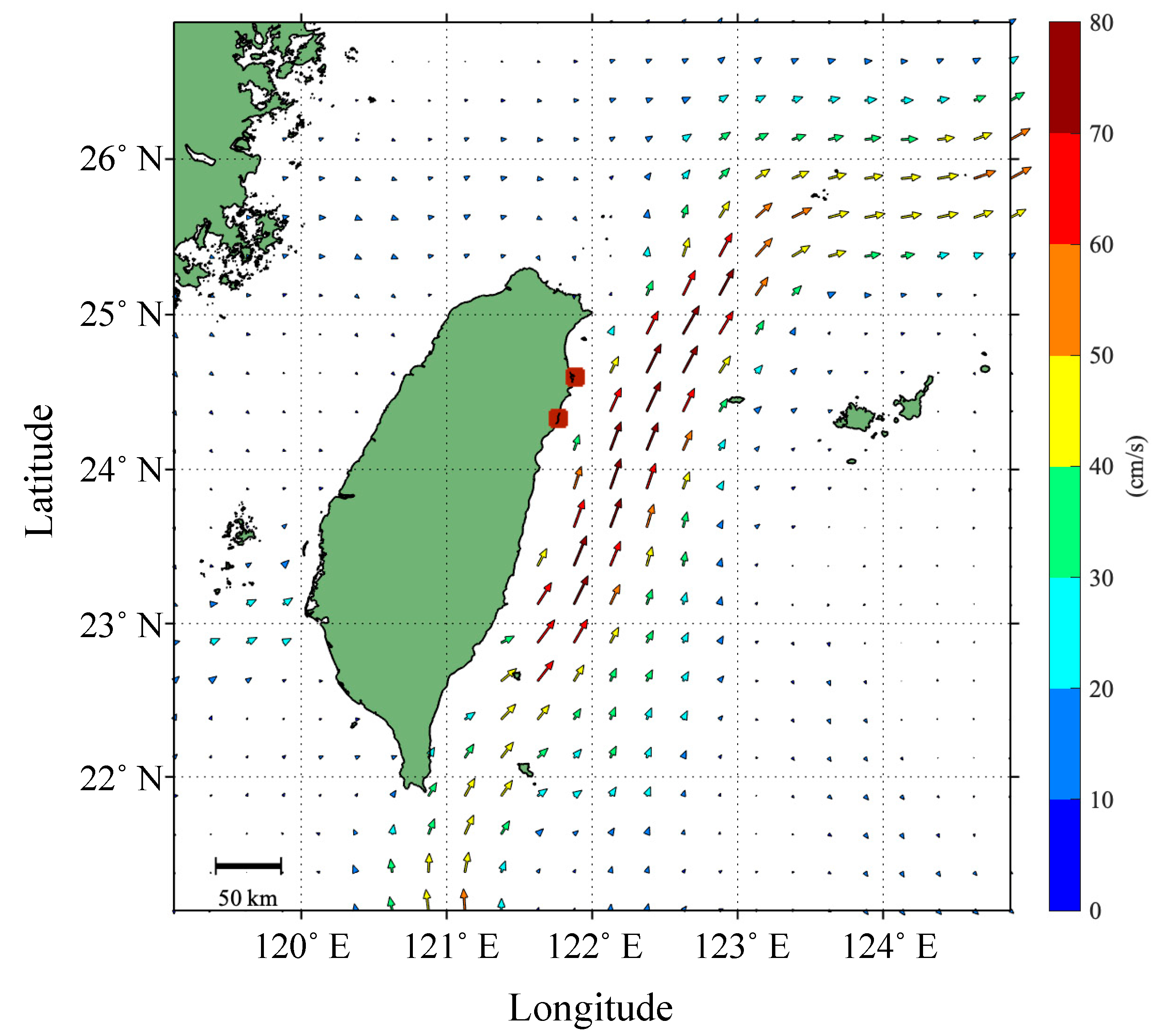
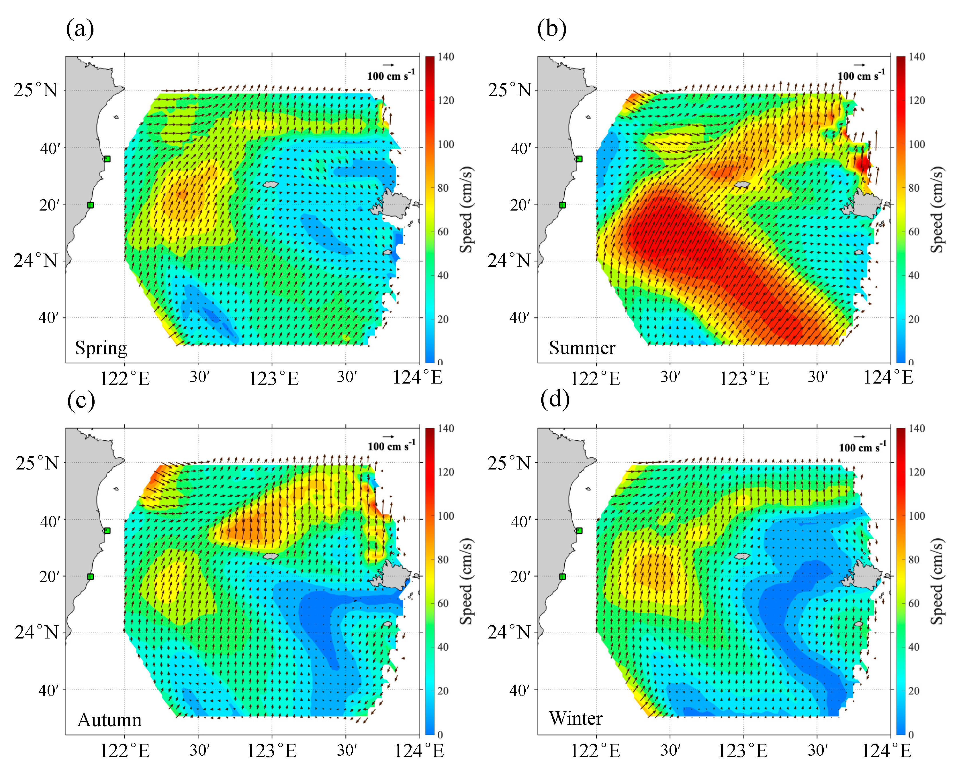
4.1. The Flow of Ocean Currents and Circulation

In this section, this study analyzes the seasonal variability of surface circulation from HFR-derived current observations. One year is divided into four seasons (spring from March to May; summer from June to August; autumn from September to November; winter from December to February). Figure 3 shows the variability in seasonal currents in the study area. The waters around Taiwan are heavily influenced by the monsoon. The large-scale wind direction and speed for the four seasons are shown in Figure 4. In winter, the northeast monsoon has strong wind speeds starting in mid-September and reaching their maximum from October to January, after which they decrease. In summer, the southwest monsoon starts at the end of May, prevails from June to July and ends in early September. In summary, the strong northeast wind, which opposes the mean current, contributes to a reduction in the surface currents measured by the HFRs in winter. In summer, the southwesterly wind blows in the same direction as the Kuroshio Current and thus increases the velocity of the Kuroshio surface currents. The change in the monsoon drives the changes in surface currents. Under the influence of complex ocean current systems, the monsoon and even topography, the mean current values for spring and autumn are 46 and 43 cm/s, respectively. Winter is the month with the lowest average flow rate of all seasons at 42 cm/s. The average flow rate in summer is 68 cm/s, with a maximum velocity of 162 cm/s (as shown in Figure 5).
The EKE values in the four seasons are shown in Figure 6. High variability can be seen in all seasons in the region of the Kuroshio at approximately 122°30′ E and 24°20′ N. There is also a meandering and higher energetic area in the northeastern region. One possible reason can be attributed to the Kuroshio flow being fastest in this area. The highest EKE values (orange region), extending from the middle to the southeast, occur in the summer. It should be noted that the amplitude of the averaged EKE is consistently smaller in the autumn and winter months than in the other months. This result is consistent with Scharffenberg and Stammer [27], who found that the maximum EKE level in the Kuroshio extension occurs in summer, while the EKE reaches its minimum there in winter. Obvious mesoscale events associated with eddies at approximately 123° E to 124° E and 23° N 40′ to 24° N 20′ occurred from autumn to winter. The main reason is that the strong Kuroshio flowing from south to north is suppressed by the northeasterly wind, and the current is impeded by the Japanese islands of Yonaguni and Iriomote, producing a clockwise mesoscale eddy. The spatial resolution of HFRs not only provides averaged current values but also reveals the fast-evolving mesoscale eddy events around Taiwan.

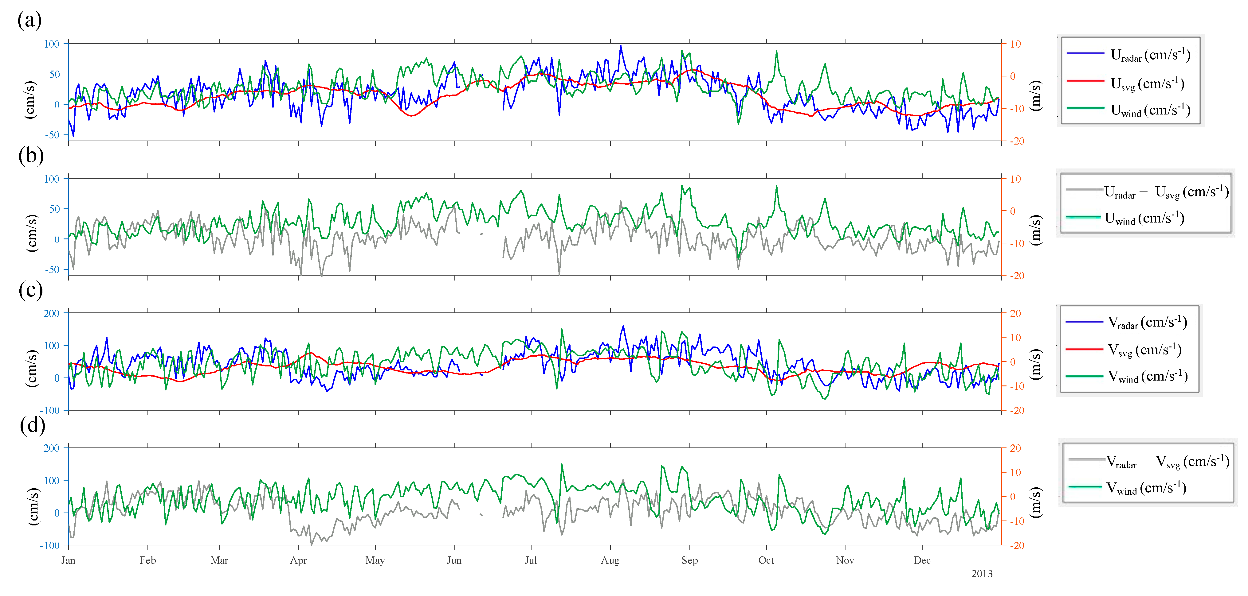
4.2. Comparison of Various Spatial Data
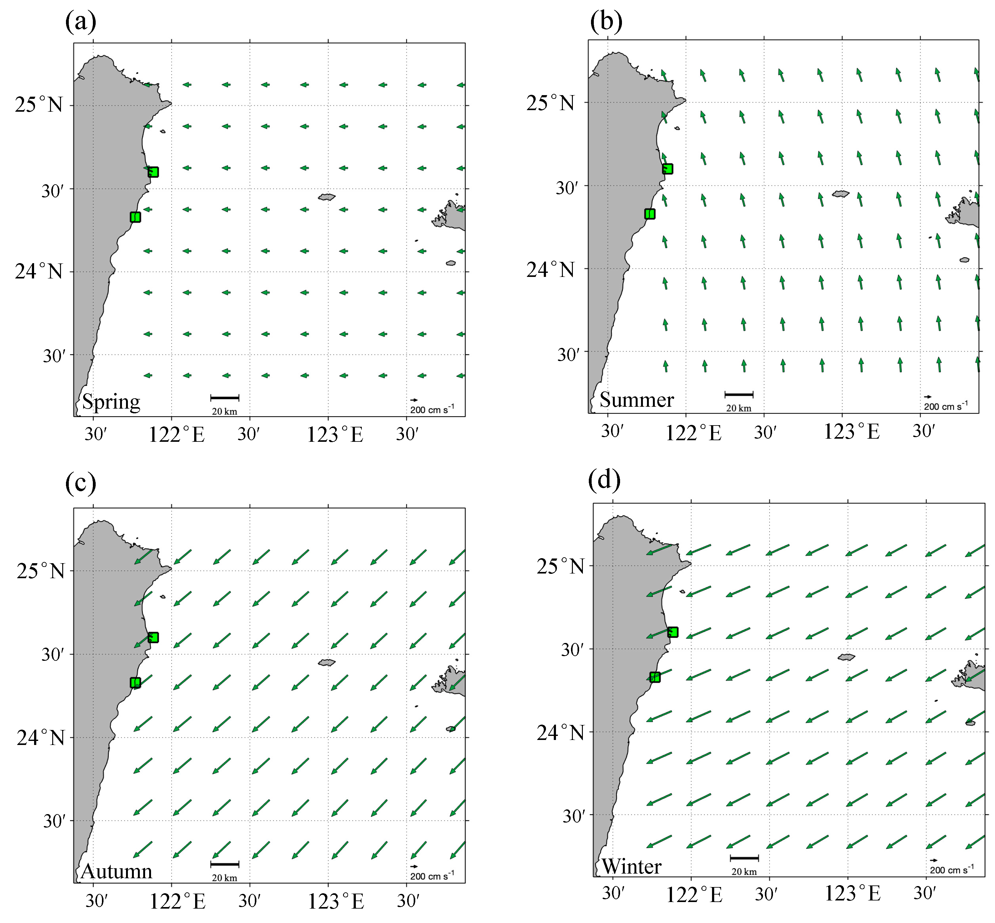
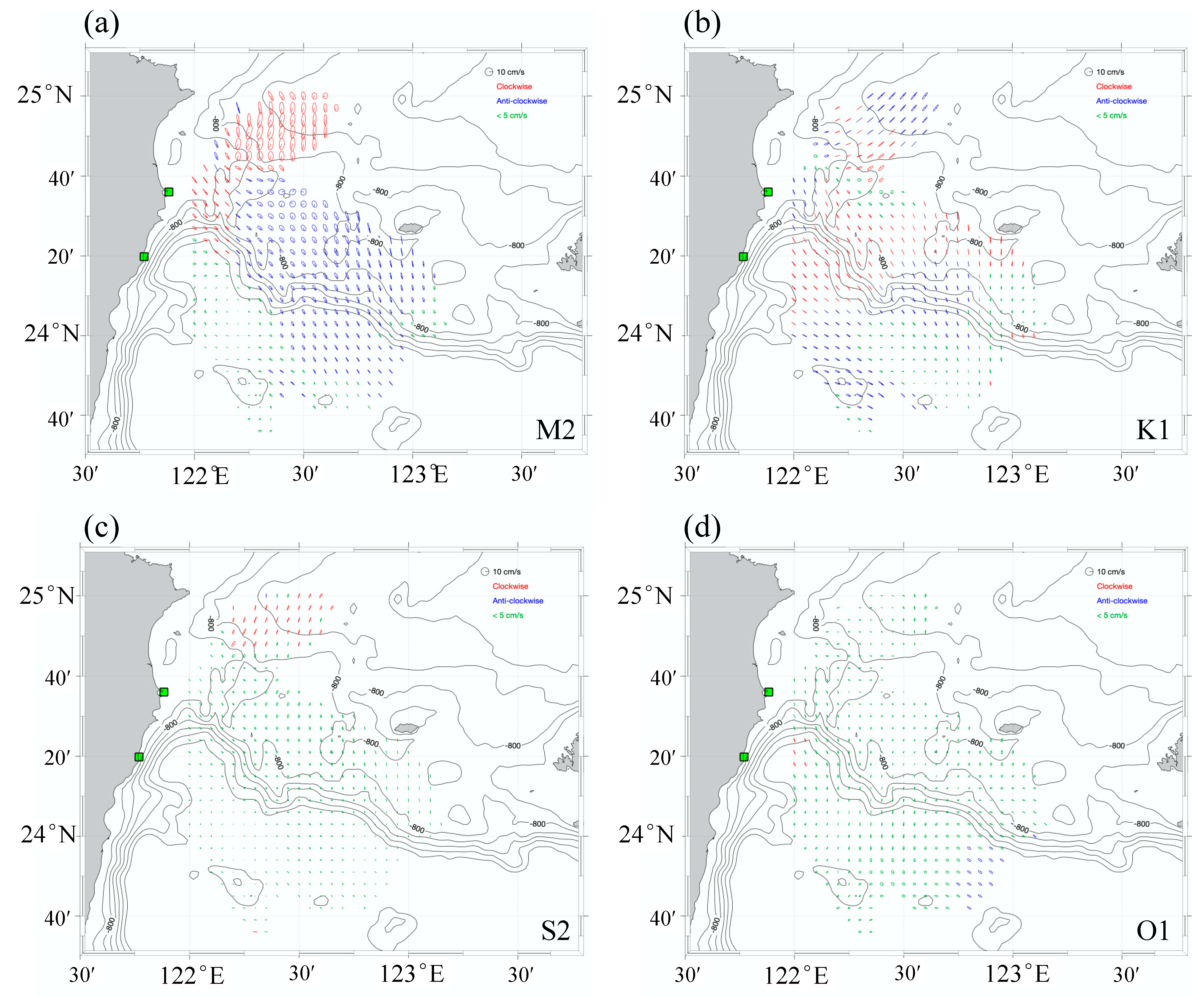
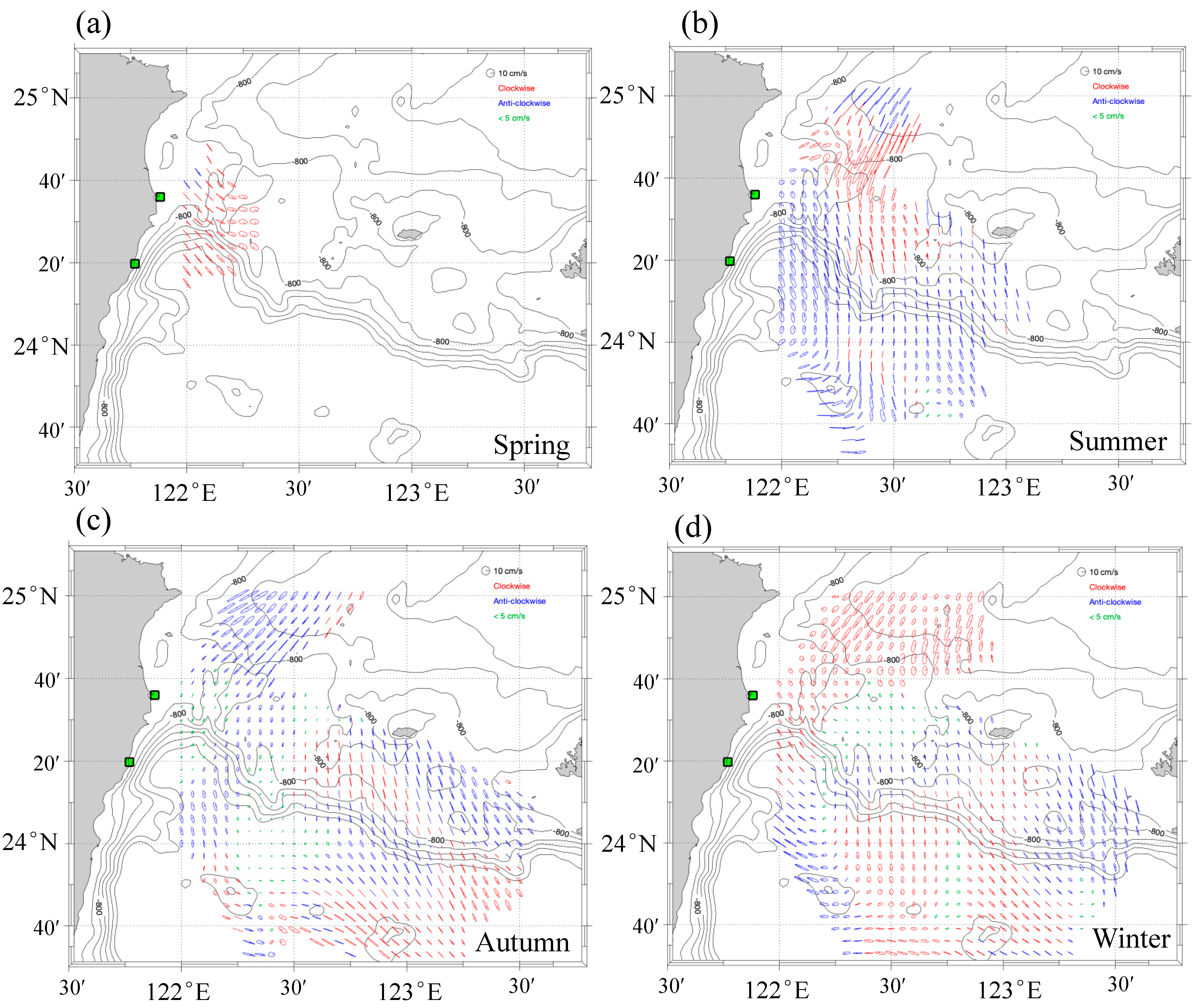
To observe the relationships among the three different variables investigated here, this study calculated complex correlations between pairs of vector time series. Figure 7 shows the annual SGV, HFR, and wind vectors in 2013, with the two grid regions selected for vector correlations indicated in Figure 7a. The red arrow is the SGV flowing from south to north; the black vector is the HFR measurement value of the sea-surface current. The orange cells are designated region of interest (ROI) 1, and the blue cells are designated ROI 2. The Kuroshio current velocity and wind speed are both relatively strong in these two areas, which is why they were selected. The wind field is approximately northeasterly throughout, as shown in Figure 7b. It is obvious that the orientation of the SGV is approximately the same as that of the current field derived by HFR, but the only difference is that HFR data include the influence of wind-driven forcing. The spatially averaged time series over the two ROIs are shown in Figure 8. The horizontal axis is time, the left vertical axis is velocity (cm/s) for the SGV and radar data, and the right vertical axis is the wind velocity (m/s). Figure 8a,b shows u component results; Figure 8c,d shows v component results. The blue line is HFR data, the red line is SGV data, and the green line is wind data. It is obvious that the component speed of the SGV (green line) behaves like a low-pass filter for the time series in Figure 8a,c due to the geostrophic effect taking place over a longer time scale. By comparison, the time series of the wind (red line) and HFR data (blue line) show high-frequency variations over shorter time scales, suggesting that wind plays an important role in directly forcing surface currents in this region. To investigate this hypothesis, this study produced a residual time series from the difference between the HFR and SGV data for surface currents. The u and v components of the wind exhibit good visual agreement with the residuals, as shown in Figure 8b,d, except for some time periods in June with missing radar data.
The results of the complex correlation of the mean wind time series against the mean HFR, SGV, and residual time series are shown in Table 3 by season for both ROI 1 and ROI 2 (see Figure 7). The correlation between the residual current and the wind vector is higher than the SGV correlation due to the geostrophic components being removed from the time series. Relative to the correlation in spring in ROI 1 and ROI 2, the radar-to-wind correlations are higher in the other three seasons due to stronger winds. In addition, the average correlation between the HFR and wind in ROI 1 is larger than that in ROI 2, with mean correlations of 0.57 and 0.49 and standard deviations (STDs) of 0.11 and 0.04 between the radar and wind, respectively. The reason for ρ1 being higher than ρ2 is likely because the islands above ROI 2 block northeasterly winds. Short time-scale wind components produce fast and variable movements in the oceans, while geostationary fields produce low-frequency phenomena on larger scales.

4.3. Tidal Flow

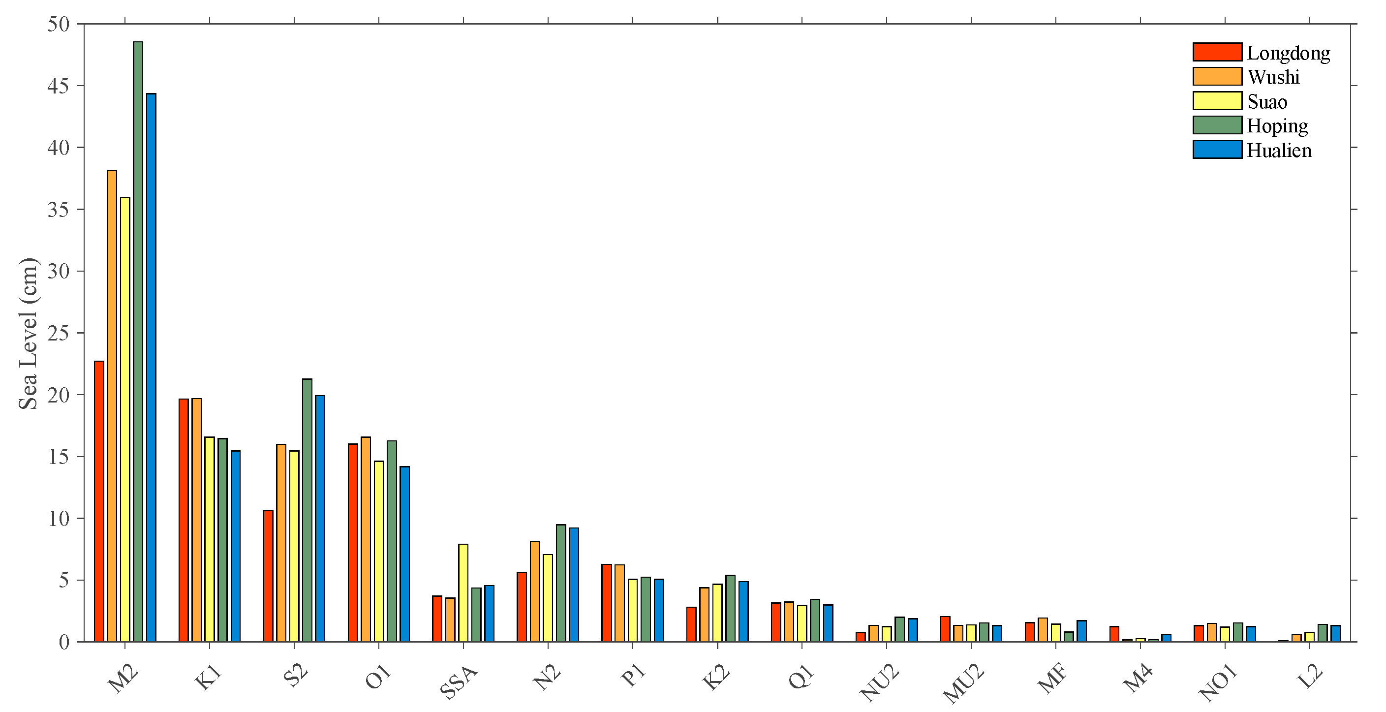
4.3.1. Validation of Tidal Constituents

In terms of tidal analysis, the tidal variation from the shallow water to the continental shelf is nonlinear, whereas in the deep ocean, it is less complex and can be analyzed by using the dominant linear dynamics of astronomical tides [28]. Off of the eastern coast of Taiwan, the continental shelf is narrow, and the water reaches a depth of 1000 m within 1–2 km of shore. Hence, the tidal interactions can be conveniently expressed as simple harmonic components with differences in phase and angular speed being multiples of astronomical constituents of M2 and S2. Tidal ellipses are the best way to represent tide-driven changes in currents, thereby describing the relationship between the u and v components [29]. This section focuses on validating the HFR-derived surface current components against those observed by coastal tide-gauge stations. Harmonic analysis of sea-surface currents is used to extract tidal components at the different locations around the HFR grid. This study quantifies the major tidal components and analyzes the tidal driving currents over the four seasons in the region off of northeastern Taiwan.
The largest semidiurnal and diurnal tidal fluctuations across the region observed by the HFRs are shown in Figure 9 as tidal ellipses resulting from harmonic analyses. These ellipses are largest at approximately 122° E to 122°30′ E and 24°40′ N to 25° N, which is located east of the Suao station. The orientations of the major axes tend to be aligned with the topography on both sides of the ridge axis, particularly for the dominant M2 and K1 constituents. Harmonic analyses of coastal surface currents close to the diurnal period can be dominated by diurnal wind forcing [4]. Here, however, the K1 ellipse alignment argues against diurnal (sea breeze) wind forcing, at least over the deep ocean ridge area. In terms of rotation, the patterns corresponding to the semidiurnal M2 and diurnal K1 ellipses are dominated by clockwise and anti-clockwise tides, respectively. In contrast, the distribution of the weaker semidiurnal S2 and diurnal O1 ellipses are observed to obtain their largest values in small patches (Figure 9c,d). Overall, the M2 tide is observed to have the highest amplitudes, and the tidal ellipses rotate in the opposite direction to K1 in the northern and central portions of the region.
The lunar synodic fortnightly (MSf) tides, with periods of 14.76 days, are typically the large tidal components at the 14-day period [30]. MSf are often contaminated with atmospheric forcing, which results in highly variable amplitudes and phases when comparing yearlong records from the same tidal station [30,31]. Schureman (1958) [32] provided the length of record (hour) with the frequency difference between neighboring constituents. Thus, the length of time needed to distinguish MSf constituents is 355 h. This study divided the data length of a year into four seasons (one season is equivalent to 3 months), so the data length is approximately 2160 h in one season, which is sufficient to distinguish MSf by season. Seasonal tidal current ellipses for MSf are shown in Figure 10. It is worth noting that the ellipse of the summer MSf constituent (Figure 10b) at approximately 122° E to 122°30′ E and 24°40′ N to 25° N is significantly larger than that in any other location or season, and all rotate counterclockwise. This may be related to the three land-proximal typhoons (Figure 11) that passed near this study area during the summer season: SOULIK, KONG-REY, and TRAMI. These observations show that these strong atmospheric systems may have had an outsized influence on these ellipses.

4.3.2. Tide Type Classification

Tidal forces can be converted into tidal potentials, and their effects can be measured through sea level fluctuations and equilibrium tide theory. Most equilibrium amplitudes are small, but there are 11 major tidal constituents, and of these, tidal analysis has shown that the four main tide constituents are M2 (principal lunar semidiurnal), S2 (principal solar semidiurnal), K1 (principal lunar diurnal), and O1 (main lunar diurnal constituent). Through these four constituents, it is possible to explain in general terms the characteristics of sea level variations, such as diurnal tides, semidiurnal tides, diurnal inequalities, spring tides and neap tides [33]. In the study region, there are five tide-gauge stations along the coast of Taiwan that measure the presence of the 15 constituents with the greatest amplitude. Those amplitudes are displayed in Figure 12 for each of the five tide-gauge locations. As expected, semidiurnal M2 and S2 and diurnal K1 and O1 exhibit the largest amplitudes. LD and HL are the northernmost and southernmost tide-gauge stations in the study area. The amplitudes of semidiurnal M2 and S2 in the northern part were smaller than those in the southern part. This result means that the semidiurnal tides are more pronounced in the south. The K1 amplitude was greater at the northern station than at the two southern stations.
To reveal the tidal characteristics and type of tide in the study area, harmonic analysis of the spatially averaged HFR currents over the entire domain was conducted for the same 15 tidal constituents (Figure 13). The high amplitudes of the long-period SSA and MF tidal constituents in the figure are almost certainly due to meteorological rather than astronomical forcing [31]. The semidiurnal (M2 and S2) and diurnal (K1 and O1) constituents, as observed from HFR currents, were compared against results from the tide-gauge observations. In previous studies, the 2D tidal current model was used to analyze the tidal characteristics of the northern Taiwan coast, and the proportion of the elliptical tidal axis was used to determine the form of the tide [34,35].
Tidal characteristics are classified according to the form ratios given in Table 4. The types of classifications based on the form ratio are taken from Courtier [36]. The form ratio represents the ratio of the sum of the amplitudes of the major diurnal components (K1 and O1) to the sum of the amplitudes of the major semidiurnal components (M2 and S2), as defined by [37]
i = K 1 + O 1 M 2 + S 2
where i is the form ratio, also known as the tidal characteristics of the criteria index.
The form ratios are given for each of the tide-gauge locations (first four columns) and the HFR surface current observations (last column) in Table 5. According to the form ratio, the tide in Taiwan is a mixed, mainly semidiurnal tide, and the results show that the tide-gauge station and HFR observations yield the same result, which is consistent with Dai et al. (2018) [38]. Most of the ocean tides are mixed, with predominantly semidiurnal tides in the northwestern Pacific Ocean and East China Sea, east of Taiwan. Moreover, these results confirm that HFR is a very good tool for tidal observation. In addition, the single time series classification is shown in Figure 13 and Table 5.

5. Discussion and Conclusions

The main focus of this paper was to investigate the current patterns, influence of wind forcing and spatial distributions of tide constituents off of northeastern Taiwan with coastal HFR systems. The results of the three subtopics are discussed below.
This study analyzes the seasonal variability of surface circulation from HFR-derived current observations. The Kuroshio flows from south to north throughout the year. In winter, the strong northeast wind blows in the opposite direction, weakening the flow of the Kuroshio surface current; in summer, the southwesterly wind accelerates the speed of the Kuroshio surface current by blowing in the same direction as the Kuroshio current. Changes in the monsoon around Taiwan drive changes in surface ocean currents. EKE results are shown for the four seasons. A high degree of variability can be seen in all seasons in the Kuroshio area at approximately 122°30′ E and 24°20′ N. There is also a windy, high-energy area in the northeast portion of the measurement area. The highest EKE values (orange area) extend from the center to the southeast and occur in summer. It should be noted that the magnitude of the average EKE is always smaller in the autumn and winter months. Regarding the observations of mesoscale events, it can also be noticed that in autumn and winter, there are obvious mesoscale eddy events in the vicinity of 123° E to 124° E and 23°40′ N to 24°20′ N. The main reason is that the strong Kuroshio current flowing from south to north is suppressed by the northeasterly wind, and the water hits Japan’s Yonaguni Island and Iriomote Island, producing a clockwise mesoscale vortex.
Sea surface currents derived from the HFR data include both SGV and wind-driven components. The result of complex correlation analysis shows that the average correlation between radar and wind and residual and wind is higher than that between SGV and wind. In addition, the correlation ρ1 of ROI 1 is higher than ρ2 of ROI 2, which may be because the island above ROI 2 blocks the northeasterly wind. This reduces the impact of the wind on the ocean currents. Since the geostrophic effect occurs on a longer time scale, the component velocity of the SGV behaves like a low-pass filter on the time series. In contrast, the wind and HFR data show high-frequency changes on a shorter time scale, indicating that wind plays an important role in directly forcing surface water flow in the area. Overall, this approach is to attempt to remove the geostrophic constituent from the HFR observations by subtracting the satellite-derived current estimates to form the residual currents. A prior study [17] followed this same approach and found that the residual currents were much better correlated with the local wind forcing than either the satellite- or HFR-derived currents. In the case of this study, there is only slight improvement in the correlation with local wind forcing for the residual currents, which suggests that there is a more complex relationship between winds and geostrophic currents in this region and/or there is significant energy in mesoscale eddies that are not wind driven but are also not resolved by the satellite measurements.
The spatial distributions of tidal ellipses in the study area were also revealed by the HFR observations. The results showed that the M2 tidal ellipses have the highest amplitudes, and the tidal ellipses rotate more than K1, S1, and O1 over the head of the I-Lan Ridge (122° E, 24°40′ N to 122°30′ E, 25° N), which is located off of the northeastern Suao station. The orientation of the major axis tends to be consistent with the topography on both sides of the ridge axis. It is worth noting that the ellipse pattern of the MSf constituent in summer is significantly larger and rotates counterclockwise at approximately 122°30′ E, 25° N. The literature records that tidal components with a period of approximately 14 days are often polluted by atmospheric forcing. The preliminary results of this study show that the three typhoons in the summer of 2013 may have forced the pattern of the MSf tidal ellipse in the summer to be different from those in the other three seasons. Moreover, according to the basic theory of tidal form ratio, the HFRs observed that the tides in Taiwan are mixed, mainly semidiurnal tides. This result is also consistent with the results from coastal tide-gauge stations.
In summary, HFRs are very good remote sensing tools to observe the characteristic motion of surrounding seas. Analyzing the available data, with particular emphasis on the higher spatial and temporal resolution of the HFR observations, this study made use of HFR observations to confirm the seasonal characteristics of current patterns, the spatial distribution of the tidal components, and the occurrence of mesoscale recirculation in the region on annual time scales. Extended coverage through an expanded HFR network over longer time periods will reveal even more regional ocean dynamics. In future studies, circulation and vorticity analyses will be beneficial to reveal more mesoscale ocean flows in the study area.

Author Contributions

Writing—original draft, Y.-R.C.; writing—review and editing, Y.-R.C., M.S.C., J.D.P., L.Z.-H.C. and Y.-J.C.; conceptualization, Y.-R.C., M.S.C., J.D.P. and L.Z.-H.C.; data curation, Y.-R.C., M.S.C. and Y.-J.C.; formal analysis, Y.-R.C., M.S.C., J.D.P. and Y.-J.C.; funding acquisition, L.Z.-H.C.; investigation, Y.-R.C., J.D.P. and L.Z.-H.C.; methodology, Y.-R.C., M.S.C., J.D.P., L.Z.-H.C. and Y.-J.C.; resources, J.D.P., L.Z.-H.C. and Y.-J.C.; software, Y.-R.C., M.S.C. and Y.-J.C.; supervision, M.S.C., J.D.P., L.Z.-H.C. and Y.-J.C.; visualization, Y.-R.C., M.S.C., J.D.P., L.Z.-H.C. and Y.-J.C. All authors have read and agreed to the published version of the manuscript.

Funding

This research was funded by the Ministry of Science and Technology under grants 109-2221-E-006-101, 109-2623-E-006-002-D, 108-2611-M-012-002, Ministry of Science and Technology Overseas Project for Post Graduate Research under grants 108-2917-I-006-012, Ministry of Education PEE1090492 and Naval Postgraduate School contributions were supported by NOAA’s Integrated Ocean Observing System agreement MOU-2020-078/12015/NPS-21-400-2778.

Institutional Review Board Statement

Not applicable.

Informed Consent Statement

Not applicable.

Data Availability Statement

The data presented in this study are available upon request from the corresponding author. The data are not publicly available due to security issues.

Acknowledgments

We thank all the scientists and principal researchers who prepared and provided the research data. Thanks to Yung-Da Sun from the Naval Meteorological and Oceano-graphic (METOC) Office R.O.C, I-Fong Tsui from Chung Cheng Institute of Technology, Yiing-Jang Yang from NTU, Chi-Min Chiu, Li-Chung Wu from Coastal Ocean Monitoring Center (COMC), Jian-Wu Lai from Ocean Affairs Council (OAC) and António Carlos Gonçalves Tavares from the Hydrographic Institute in portugal for discussion and technique support. We would also like to thank the Central Weather Bureau (CWB), Ministry of Transportation and Communications who provided tide gauge data to our research. Last but not least, we also thank the anonymous reviewers for their constructive observations.

Conflicts of Interest

The authors declare no conflict of interest.

References

  1. Yang, Y.; Liu, C.-T.; Hu, J.-H.; Koga, M. Taiwan Current (Kuroshio) and impinging eddies. J. Oceanogr. 1999, 55, 609–617. [Google Scholar] [CrossRef]
  2. Liang, W.-D.; Tang, T.; Yang, Y.; Ko, M.; Chuang, W.-S. Upper-ocean currents around Taiwan. Deep Sea Res. Part II Top. Stud. Oceanogr. 2003, 50, 1085–1105. [Google Scholar] [CrossRef]
  3. Paduan, J.D.; Washburn, L. High-frequency radar observations of ocean surface currents. Annu. Rev. Mar. Sci. 2013, 5, 115–136. [Google Scholar] [CrossRef] [PubMed] [Green Version]
  4. Paduan, J.D.; Cook, M.S. Mapping surface currents in Monterey Bay with CODAR-type HF radar. Oceanography 1997, 10, 49–52. [Google Scholar] [CrossRef] [Green Version]
  5. Lee, B.C.; Fan, Y.M.; Doong, D.J.; Kao, C.C. A study on the homogeneity of tides around coasts of Taiwan. J. Mar. Eng. 2005, 5, 67–83. [Google Scholar]
  6. Yoshikawa, Y.; Masuda, A.; Marubayashi, K.; Ishibashi, M. Seasonal variations of the surface currents in the Tsushima Strait. J. Oceanogr. 2010, 66, 223–232. [Google Scholar] [CrossRef]
  7. Yoshikawa, Y.; Masuda, A. Seasonal variations in the speed factor and deflection angle of the wind-driven surface flow in the Tsushima Strait. J. Geophys. Res. Oceans 2009, 114. [Google Scholar] [CrossRef]
  8. Fang, Y.C.; Wang, J.; Yang, Y.J. Surface Current Measurement Using HF-Radar off Northeastern Taiwan: Preliminary Result and Validation. In Proceedings of the 1st Ocean Radar Conference for Asia, Seoul, Korea, 17–19 May 2012; pp. 45–48. [Google Scholar]
  9. Chen, Y.-W.; Yang, Y.J.; Wang, J. A study on data filling from incomplete dataset of HF radar measured ocean currents—A case study of the flow field Northeast of Taiwan: Data filling from incomplete ocean currents dataset. In Proceedings of the OCEANS 2014, Taipei, Taiwan, 7–10 April 2014; pp. 1–4. [Google Scholar]
  10. Picot, N.; Case, K.; Desai, S.; Vincent, P.; Bronner, E. AVISO and PODAAC User Handbook. IGDR and GDR Jason Products; Jet Propulsion Laboratory, California Institute of Technology: Pasadena, CA, USA, 2003. [Google Scholar]
  11. Hsin, Y.C.; Qiu, B.; Chiang, T.L.; Wu, C.R. Seasonal to interannual variations in the intensity and central position of the surface Kuroshio east of Taiwan. J. Geophys. Res. Oceans 2013, 118, 4305–4316. [Google Scholar] [CrossRef]
  12. Chao, S.-Y. Circulation of the East China Sea, a numerical study. J. Oceanogr. 1990, 46, 273–295. [Google Scholar] [CrossRef]
  13. Roesler, C.J.; Emery, W.; Kim, S.Y. Evaluating the use of high-frequency radar coastal currents to correct satellite altimetry. J. Geophys. Res. Oceans 2013, 118, 3240–3259. [Google Scholar] [CrossRef] [Green Version]
  14. Scott, J.; Wentz, F.; Hoffman, R.; Atlas, R. Improvements and Advances to the Cross-Calibrated Multi-Platform (CCMP) Ocean Vector Wind Analysis (V2. 0 release). Am. Geophys. Union 2016, 2016, PO54F-3322. Available online: https://www.researchgate.net/publication/298552723_Improvements_and_Advances_to_the_Cross-Calibrated_Multi-Platform_CCMP_Ocean_Vector_Wind_Analysis_V20_release (accessed on 27 August 2021).
  15. Richardson, P.L. Eddy kinetic energy in the North Atlantic from surface drifters. J. Geophys. Res. Oceans 1983, 88, 4355–4367. [Google Scholar] [CrossRef]
  16. Sikhakolli, R.; Sharma, R.; Basu, S.; Gohil, B.; Sarkar, A.; Prasad, K. Evaluation of OSCAR ocean surface current product in the tropical Indian Ocean using in situ data. J. Earth Syst. Sci. 2013, 122, 187–199. [Google Scholar] [CrossRef] [Green Version]
  17. Reyes Suarez, N.C.; Cook, M.S.; Gačić, M.; Paduan, J.D.; Drago, A.; Cardin, V. Sea Surface Circulation Structures in the Malta-Sicily Channel from Remote Sensing Data. Water 2019, 11, 1589. [Google Scholar] [CrossRef] [Green Version]
  18. Kim, S.Y.; Cornuelle, B.D.; Terrill, E.J. Anisotropic response of surface currents to the wind in a coastal region. J. Phys. Oceanogr. 2009, 39, 1512–1533. [Google Scholar] [CrossRef] [Green Version]
  19. Kohut, J.T.; Glenn, S.M.; Paduan, J.D. Inner shelf response to tropical storm Floyd. J. Geophys. Res. Oceans 2006, 111. [Google Scholar] [CrossRef]
  20. Paduan, J.D.; Rosenfeld, L.K. Remotely sensed surface currents in Monterey Bay from shore-based HF radar (Coastal Ocean Dynamics Application Radar). J. Geophys. Res. Oceans 1996, 101, 20669–20686. [Google Scholar] [CrossRef]
  21. Kundu, P.K. Ekman veering observed near the ocean bottom. J. Phys. Oceanogr. 1976, 6, 238–242. [Google Scholar] [CrossRef]
  22. Kohut, J.T.; Glenn, S.M.; Chant, R.J. Seasonal current variability on the New Jersey inner shelf. J. Geophys. Res. Oceans 2004, 109. [Google Scholar] [CrossRef] [Green Version]
  23. Rosenfeld, L.; Shulman, I.; Cook, M.; Paduan, J.; Shulman, L. Methodology for a regional tidal model evaluation, with application to central California. Deep Sea Res. Part II Top. Stud. Oceanogr. 2009, 56, 199–218. [Google Scholar] [CrossRef]
  24. de Beurs, K.M.; Henebry, G.M. Spatio-temporal statistical methods for modelling land surface phenology. In Phenological Research; Springer: Berlin/Heidelberg, Germany, 2010; pp. 177–208. [Google Scholar]
  25. Pawlowicz, R.; Beardsley, B.; Lentz, S. Classical tidal harmonic analysis including error estimates in MATLAB using T_TIDE. Comput. Geosci. 2002, 28, 929–937. [Google Scholar] [CrossRef]
  26. Britannica, T. Harmonic Analysis. Available online: https://www.britannica.com/science/harmonic-analysis (accessed on 27 August 2021).
  27. Scharffenberg, M.G.; Stammer, D. Seasonal variations of the large-scale geostrophic flow field and eddy kinetic energy inferred from the TOPEX/Poseidon and Jason-1 tandem mission data. J. Geophys. Res. Oceans 2010, 115. [Google Scholar] [CrossRef] [Green Version]
  28. Madah, F.; Mayerle, R.; Bruss, G.; Bento, J. Characteristics of tides in the Red Sea region, a numerical model study. Open J. Mar. Sci. 2015, 5, 193. [Google Scholar] [CrossRef] [Green Version]
  29. Subeesh, M.; Unnikrishnan, A.; Fernando, V.; Agarwadekar, Y.; Khalap, S.; Satelkar, N.; Shenoi, S. Observed tidal currents on the continental shelf off the west coast of India. Cont. Shelf Res. 2013, 69, 123–140. [Google Scholar] [CrossRef]
  30. Ponte, R.M.; Chaudhuri, A.H.; Vinogradov, S.V. Long-period tides in an atmospherically driven, stratified ocean. J. Phys. Oceanogr. 2015, 45, 1917–1928. [Google Scholar] [CrossRef]
  31. Crawford, W. Analysis of fortnightly and monthly tides. Int. Hydrogr. Rev. 1982, LIX, 132–141. [Google Scholar]
  32. Schureman, P. Manual of Harmonic Analysis and Prediction of Tides; US Government Printing Office: Washington, DC, USA, 1958; Volume 4. [Google Scholar]
  33. Stewart, R.H. Introduction to Physical Oceanography; Texas A&M University: College Station, TX, USA, 2008. [Google Scholar]
  34. Lin, S.F.; Yang, Y.J.; Tang, T.Y. Coastal Tidal Current Phenomena on Northern Taiwan. In Proceedings of the 27th Ocean Engineering Conference, Taichung, Taiwan, 1–2 December 2005. [Google Scholar]
  35. Dietrich, G.; Kalle, K. General Oceanography; An Introduction; Interscience Pub.: New York, NY, USA, 1957. [Google Scholar]
  36. Courtier, A. Classification of tides in four types. Int. Hydrogr. Rev. 1939. Available online: https://journals.lib.unb.ca/index.php/ihr/article/download/27428/1882520184 (accessed on 27 August 2021).
  37. Hicks, S.D. Tidal wave characteristics of Chesapeake Bay. Chesap. Sci. 1964, 5, 103–113. [Google Scholar] [CrossRef]
  38. Dai, C.F. Regional Oceanography of Taiwan Version II; National Taiwan University Press: Taipei, Taiwan, 2018. [Google Scholar]
Figure 1. The surface current data coverage in percentages (%) in 2013. Green squares indicate the Suao and Habn HFR stations. The red triangles indicate the tide-gauge stations along the coastline. The island in the center and the island closest to the eastern edge of the domain are the Japanese islands of Yonaguni and Iriomote, respectively. The black box inside the inset at the bottom left represents the study area.
Remotesensing 13 03438 g001
Figure 2. Mean surface geostrophic velocity (SGV) in 2013.
Remotesensing 13 03438 g002
Figure 3. Seasonal current velocities (vectors) in the region off of northeastern Taiwan. The green point in the north is the SUAO station, and the southern point is the HABN station; the flow direction is indicated by the arrow vectors, and the contour plots of velocities are for the flow rates. (a) Spring, (b) Summer, (c) Autumn, and (d) Winter.
Remotesensing 13 03438 g003
Figure 4. Wind fields for the four seasons off eastern Taiwan. The wind direction reverses between winter and summer, whereas the wind is basically from the northeast in winter and autumn. (a) Spring, (b) Summer, (c) Autumn, and (d) Winter.
Remotesensing 13 03438 g004
Figure 5. Box plots of the sea-surface currents for the four seasons. A five-value summary is shown for each dataset, including the minimum, first (lower) quartile, median (red line), third (upper) quartile, and maximum.
Remotesensing 13 03438 g005
Figure 6. Seasonal current velocities (vectors) in the region off of northeastern Taiwan with the EKE (background color). (a) Spring, (b) Summer, (c) Autumn, and (d) Winter.
Remotesensing 13 03438 g006
Figure 7. Mean SGV, HFR, and wind vectors from 1 January 2013 to 31 December 2013. (a) The red arrows are the SGV flowing from south to north; the black vectors are HFR measurements of the sea-surface current. The two grid regions where complex correlations are computed for box-averaged currents are also shown with the orange cell designated ROI 1 and the blue cell designated ROI 2. (b) Mean wind velocities, which are from the northeast.
Remotesensing 13 03438 g007
Figure 8. Spatially averaged u and v components of the daily wind, SGV and HFR velocity time series related to box 1 (a,b) and box 2 (c,d).
Remotesensing 13 03438 g008
Figure 9. (a) M2, (b) K1, (c) S2, and (d) O1 tidal ellipses derived from harmonic analysis of the HFR current data. The red (blue) ellipses indicate clockwise (anti-clockwise) rotation. The green ellipses indicate tide speeds of less than 5 cm/s. The thick black line is the −800 m isobath.
Remotesensing 13 03438 g009
Figure 10. Current tidal ellipses for harmonic constituent MSf. (a) Spring, (b) Summer, (c) Autumn, and (d) Winter.
Remotesensing 13 03438 g010
Figure 11. Three typhoons passed to the east and north of the study area during the summer period.
Remotesensing 13 03438 g011
Figure 12. Amplitudes of sea level height (in cm) based on instrument reference level (RL) for 15 constituents from five tide-gauge stations from north to south in sequence.
Remotesensing 13 03438 g012
Figure 13. The mean current ellipse major axis magnitude (in cm/s) for 15 constituents from the HFR over the entire domain.
Remotesensing 13 03438 g013
Table 1. Summary of the key dataset characteristics.
HFRAltimeter (Aviso+)CCMPETOPO1Tide Gauge
VariableSea surface velocitiesGeostrophic currentWind stressBathymetrySea level
Temporal resolutionHourlyDaily6-hourly Hourly
Spatial resolution1/13°1/8°1/4°1/60°
Vertical integration1 m under the surfaceSurface10 m above sea levelDegree of depthInstrument reference level
Table 2. Operating parameters of the study area HFRs.
ParameterValue
Radar frequency (fc)4.4 MHz
Sweep bandwidth (B)18.38 kHz
Sweep period or sweep repetition time (Ts)1 s
Range resolution (c/2B)8.16 km
Maximum range292 km
Sampling time243.2 μs
Table 3. Complex correlation coefficients and veering angles of the HFR, SGV, and residual data with the wind in four seasons.
2013Geostrophic to WindRadar to WindResidual to Wind
ρ1ρ2θ1θ2ρ1ρ2θ1θ2ρ1ρ2θ1θ2
Spring0.350.34−111.76−128.990.420.44−151.33−87.260.460.48110.46−12.35
Summer0.400.37−47.57−45.760.500.50−81.79−45.460.510.48−178.66−60.90
Autumn0.320.37−163.51−140.080.670.45177.87−132.290.460.4072.99−100.76
Winter0.400.39−130.21−110.700.690.55−138.33−105.910.480.50112.58−99.79
Mean0.370.37−113.26−106.380.570.49−48.40−92.730.480.4729.34−68.45
STD0.030.0242.2236.540.110.04133.2231.630.020.04121.1231.16
Table 4. Classification types of tidal characteristics.
Form RatioType
0.00–0.25Semidiurnal tide
0.25–1.50Mixed mainly semidiurnal tide
1.50–3.00Mixed mainly diurnal tide
3.00–∞Diurnal tide
Table 5. Results of the form ratio and tidal patterns from the tide-gauge stations and HFR.
LDWSSOHPHLCODAR
Form ratio1.06900.670240.605990.468490.460570.91193
Tidal typesMixed mainly semidiurnal tide
Publisher’s Note: MDPI stays neutral with regard to jurisdictional claims in published maps and institutional affiliations.

