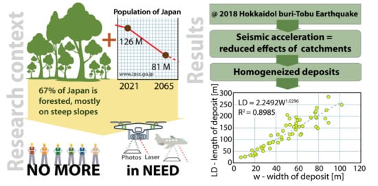
Deposits’ Morphology of the 2018 Hokkaido Iburi-Tobu Earthquake Mass Movements from LiDAR & Aerial Photographs

Abstract

On 6 September at 03:08 a.m. local time, a 33 km deep earthquake underneath the Iburi mountains triggered more than 7000 co-seismic mass movements within 25 km of the epicenter. Most of the mass movements occurred in complex terrain and became coalescent. However, a total of 59 mass movements occurred as discrete events and stopped on the semi-horizontal valley floor. Using this case study, the authors aimed to define planar and vertical parameters to (1) compare the geometrical parameters with rain-triggered mass movements and (2) to extend existing datasets used for hazards and disaster risk purposes. To reach these objectives, the methodology relies on LiDAR data flown in the aftermath of the earthquake as well as aerial photographs. Using a Geographical Information System (GIS), planform and vertical parameters were extracted from the DEM in order to calculate the relationship between areas and volume, between the Fahrböschung and the volume of the deposits, and to discuss the relationship between the deposit slope surface and the effective stress of the deposit. Results have shown that the relation $S=k{\left[V_d\right]}^{2/3}$ (where S is the surface area of a deposit and V_d the volume, and k a scalar that is function of S) is k = 2.1842ln(S) − 10.167 with a R² of 0.52, with less variability in deposits left by valley-confined processes compared to open-slope processes. The Fahrböschung for events that started as valley-confined mass-movements was Fc = −0.043ln(D) + 0.7082, with a R² of 0.5, while for open-slope mass-movements, the Fo = −0.046ln(D) + 0.7088 with a R² of 0.52. The “T-values”, as defined by Takahashi (2014), are displaying values as high as nine times that of the values for experimental rainfall debris-flow, signifying that the effective stress is higher than in rain-triggered counterparts, which have an increased pore pressure due to the need for further water in the material to be moving. For co-seismic debris-flows and other co-seismic mass movements it is the ground acceleration that “fluidizes” the material. The maxima found in this study are as high as 3.75.

1. Introduction

The world population is increasingly urban, leaving vast areas of ‘green deserts’ which are sometimes located at the door-step of human settlements. In Hong-Kong, for instance, the proximity of the two has led to numerous mass movements taking the lives of more than 470 people since the 1940s [1]. As a consequence, civil engineers have developed and implemented numerous geometric relationships, such as the angle of repose, to assess the hazardous zones (e.g., in Hong-Kong, China [2]).

Although geotechnical engineering is arguably a preferable approach, in remote areas and in countries where the population or the budget are decreasing, it has become essential to develop different methods which rely on lower-cost automated systems that can contribute to the further development of statistical approaches. For example, the database analytics of the Enhanced Natural Terrain Landslide Inventory (ENTLI), which has 19,763 records in Hong-Kong, can contribute to developing such approaches [3].

Furthermore, the Covid19 crisis, which has swept across the world, has temporarily impaired travel to the field, emphasizing the importance of working with remote sensing data. Within this framework, the present contribution proposes a remote-sensing approach to the morphological parameters of the individual co-seismic mass-movements triggered during the Hokkaido Iburi-Tobu (HIT) Earthquake, discussing their specificity to seismic-triggering.

1.1. The 2018 Hokkaido Iburi-Tobu (HIT) Earthquake and the Coseismic Mass-Movements

On 5 September 2018 at 18:07 UTC (6 September at 03:08AM local time), a magnitude 6.6 earthquake shook the Iburi-Tobu region, south of Hokkaido, Japan (Figure 1). The shallow earthquake (33 km depth) was the result of a reverse-slip fault movement, which resulted in 7059 mass movements (Figure 1) within an area of 466 km² [4]. Furthermore, remote sensing-based spatial analysis has shown that the density of mass-movements was up to 95 [number/km²] [5], and that this density was related to the surface area by the relationship:

$$\mathrm{y}=110 {\ast \mathrm{e}}^{[-\log \left(\mathrm{x}\right)-\frac{3.26{)}^2}{0.2378}]}$$

(1)

where y is the number of mass movement for a given x surface area [4].

The large number and high-density of mass-movements can be first explained by the seismic and geologic realm of the event. The earthquake is believed to be the result of a local crustal weakness, which reacted to the regional strain accumulation [6]. The sudden energy release is supposed to have originated from a major slip along the faulting plane [7,8]. This subterranean slip then translated at the surface into strong motion, notably under the amplification of the near-subsurface structure [9]. The near-subsurface is made of +/−9000 years old air-fall lapilli-sized pumice soil layers (about 1.5 m thick). This formation draped the Neogene sediment [10], creating a stratigraphic discontinuity. This discontinuity explains the majority of shallow landslides which move on planes parallel to the surface (Figure 1(1–5)).

Besides the geological factors, heavy antecedent rainfalls that occurred before the earthquake contributed to destabilizing the slopes. The HIT earthquake occurred one day after Typhoon Jebi (Typhoon 21 of the year 2018) had swept over the area, pouring a cumulative rainfall of 100 mm over three days [10]. One can then logically assume that the slope shear strength was weakened before the HIT earthquake occurred.

Because of the combination of both the typhoon and the earthquake, scientists have proposed that one of the two parameters were at the origin of the high number and density of mass movements. However, due to the local variation and temporal variation of mechanical properties of the soil, physically-based deterministic models remain elusive to scientists who have to work statistically from databases [11]. Consequently, the present work aims:

(1)

to contribute to existing databases of the morphology of mass-movement deposits and how they relate to the watershed morphometry they flow in (e.g., ENTLI in Hong-Kong, or in Taiwan after the Typhoon Morakot) [12];

(2)

to provide an insight into the 3D geometrical relationships of the deposits in the area impacted by the HIT-earthquake, as existing work has been so far focused on the spatial distribution of the events and the 2D characterization of the mass-movement deposits.

This research finds further motivation in the fact that most mass movements are either rainfall-triggered or seismically-triggered, but are occasionally the result of these two factors combined, for which further research is needed [13,14] even in areas of relatively low seismic activity [5].

1.2. The Mapping of Mass-Movements from Aerial Remote-Sensing Platforms

Mass-movements can be either very slow and deep-seated [15] or more shallow events, such as rotational, planar slides, rock falls or debris flows [16], displaying surface deformation at a variety of scales (from the entire mountain down, to a few meters across). For the study of mass-movements, there exists a broad range of remote-sensing platforms. They range from satellite [17,18] down to airborne, UAV and Ground-based laser techniques and photogrammetry [19]. Although remote-sensing is now sufficiently developed to generate datasets without contact-data, aerial photo-analysis, for instance, has long been considered to be a complement to field surveys [20]. Even methods that have gained prominence in recent years, such as structure-from-motion from aerial photographs [21,22] and UAV [23], still need to incorporate ground control data [24,25,26]. Remote sensing has therefore considerably helped the field of detection and mapping of mass movements, even if there is still scope to develop the method further for disaster-risk research [27]. Because understanding of the physics of mass movements is still in its infancy, remote sensing is an essential method for broadening the available databases on the geometry and precursory signs of mass movements. These indicators can then be used in hazards and disaster risk research. These geometric characteristics can then be used to improve empirical models for hazard and disaster risk management.

1.3. Empirical Relationships for Mass-Movements

Using remote-sensing platforms and field surveys, scientists have emphasized the generation of descriptive and explanatory metrics which describe the morphology of the triggering zones and deposits. Such metrics are essential to compare mass-movements between events and between one location and another. In Greece, for instance, remote sensing has allowed the construction of a database covering events that span 72 years [28].

For the present study, the mass movements of the HIT earthquake are mostly shallow rapid-onset events, involving a mixture of soils and wood debris (Figure 1). These characteristics relate the events to either debris-flows or debris-avalanches, which have been defined as: “rapid to extremely rapid shallow flow of partially or fully saturated debris on a steep slope, without confinement in an established channel” [29].

For the characterization of mass movement deposits, and especially debris flows, researchers have developed a set of morphological metrics [28], such as the repose angle that can also be expressed as the H/L (Height / Length) of the mass movement [2]. Scheidl and Rickenmann [30] have expressed the relationship between the deposit basal area S and the volume V using the following relation:

$$\mathrm{S}={{\mathrm{K}}^{\prime }}_{\mathrm{B}}{\mathrm{V}}^{\mathsf{\beta }}$$

(2)

where $\mathrm{S}$ is the basal area of the deposit, ${\mathrm{V}}^{\mathsf{\beta }}$ is the volume of the deposit and ${{\mathrm{K}}^{\prime }}_{\mathrm{B}}$ is a constant. For this expression, Crosta et al. [31] determined ${\mathrm{V}}^{\mathsf{\beta }}$ to be 2/3, and ${{\mathrm{K}}^{\prime }}_{\mathrm{B}}$ to be equal to 6.2. This equation comes from two power–law relations between the size of the deposit and the volume on one hand, and between the flow cross-section and the volume of the deposit on the other hand [32].

On top of the planform relation of the deposit, other indicators relate the deposit to the geometry of the catchment where the mass-movement started. The most concise approach links the vertical and horizontal translation to the volume of the mass transported, providing an empirical assessment of potential hazards. This relation has been famously expressed as the Fahrböschung, which is expressed as the angle between the highest starting point of a mass movement, and the furthest point the translated mass reaches. Other empirical relations have similarly linked the travel angle, starting from the center of the gravity of the mass to be translated (before sliding) to the center of the mass of the deposit [33]. For the volume of 1 × 10² m³ to 1 × 10⁶ m³ from Swiss debris flow, the travel angle—tan β—varied between less than 0.1 to 0.8, with a trend showing a decrease in the travel angle with the increase of the volume of the debris flows [33]. However, the variability in the dataset means that it cannot operate as a prediction tool on its own, as the tan β varies from 0.2 to > 0.6 for 1 × 10³ m³ for the debris flow and from < 0.1 to 0.5 for debris flows around 1 × 10⁵ m³ volume. Rock avalanches and mass movements also show similar patterns, however they indicate a different relationship between the two variables [34]. These relations were formulated by Corominas [33] as:

$$\log \left(\frac{\mathrm{H}}{\mathrm{L}}\right)=-1.05\log \mathrm{V}-0.012$$

(3)

where H is the vertical difference and L the horizontal distance and V the volume, and in a different form, Rickenmann [35] found a relation with R² = 0.75 for 160 debris flows expressed as:

$$\mathrm{L}=1.9{\mathrm{V}}^{0.16}{\mathrm{H}}^{0.83}$$

(4)

Therefore, from the Northern American mountains to the European, New-Zealand and Japanese Alps, an abundance of debris-flows have been instrumental in developing these empirical relationships.

Building on this legacy of shape-factors construction, the present research contributes a set of geometric relationships for mass movements triggered by a combination of rainfall and seismic activity. The working hypothesis has been that the effects of the watershed morphological characteristics should be partially limited, creating a homogeneous dataset, due to the continuous liquefaction of the material from the seismic acceleration.

For the present contribution, the objective is therefore to calculate geometric relations for the mass movements triggered by the 2018 HIT Earthquake, using aerial photographs and LiDAR data.

2. Methodology

To create unbiased and comparable geometric relations of each mass movement, the mass movements sampled for the present study: (1) do not overlap with one another, because it is difficult to determine how one mass movement influenced the other, and; (2) do not run-up complex slopes, as once again the quantification of these effects is difficult to achieve with remote sensing. As such, the present work selected mass movements that (1) were not coalescent, and; (2) did not run up on an adjacent slope, but stopped on a flat valley floor. Based on these parameters, 59 mass movements were identified and used in the present study.

2.1. Data Acquisition: Information Retrieval from Lidar and Aerial Photographs Using GIS

The present contribution relies on orthophotographs (10 cm resolution) created from aerial photographs taken in the immediate aftermath of the earthquake and a LiDAR-based DEM. The gridded DEM is 52,000 × 45,000 pixels. Each pixel is 0.5 m × 0.5 m in size, and the DEM is projected in JGD2011. The aerial photographs’ resolution is 0.1 m × 0.1 m. Both datasets were produced by the Japanese Government Ministry of Land Infrastructure and Transport.

In the QGIS environment, shapefiles were used to delineate the planform of the mass-movement deposits and make calculations over the raster images. For each mass-movement, the following planform data was acquired: the total travel distance (L), the width of the mass movement deposits (W), and the length of the deposits (LD). Vertical data are composed of: the elevation difference between the crown of the mass-movement and the toe of the deposit (H), the height difference between the upstream elevation and the apex elevation (B), and the mean elevation of the deposit (Figure 2).

The parameters were then combined geometrically in order to estimate the volume of deposits V, with Z and B, respectively representing the vertical and horizontal components of the volume downstream of the slope break (Equation (5)):

$$\mathrm{V}={\displaystyle \sum }_{\mathrm{i}=1}^{\mathrm{n}}{\mathrm{Z}}_{\mathrm{i}}-{\displaystyle \sum }_{\mathrm{i}=1}^{\mathrm{n}}{\mathrm{B}}_{\mathrm{i}}$$

(5)

To calculate the Fahrböschung (which is given here as simply the ratio of the height to the distance travel), we used the following relation:

$$\mathrm{F}=\frac{\mathrm{Ht}-\mathrm{Hb}}{\mathrm{L}}$$

(6)

The Fahrböschung is often expressed in degrees, but in the text we refer to H/L as the Fahrböschung (the reader can transform it into an angle when suited).

2.2. Empirical Analysis

After creating the geometric indicators, the next methodological step is an empirical analysis of the relations between the different morphological factors. This analysis relies on geometric equations and the power-law by Crosta et al. [31] expressed as:

$$\mathrm{S}={\mathrm{kV}}_{\mathrm{d}}{}^{2/3}$$

(7)

where S is the surface area of the deposit, and V_d is the volume of the deposit, with k being a scalar depending on the type of flow and the event recorded. Using the empirical data generated by remote sensing, the value(s) of k has been calculated and compared to the geometrical parameters of the mass movements to measure the variability of the k parameter between mass movements of different geometries.

Another scalar that was investigated is the scalar that was developed for rain-triggered debris-flows, which seems to apply well to the present problem as the deposits have been described as “debris-flow-like” [4] and because the relation relates the fanning surface A and the volume of the debris-flow [36] so that it can be extracted from the deposits morphology:

$$\mathrm{T}=\frac{{\mathrm{V}}_{\mathrm{d}}}{{\mathrm{S}}^{\raisebox{1ex}{$3$}\!\left/ \!\raisebox{-1ex}{$2$}\right.}\tan \left({\mathsf{\gamma }}_{\mathrm{d}}-{\mathsf{\theta }}_{\mathrm{d}}\right)}$$

(8)

where T = 5/12 for debris-flows, ${\mathsf{\gamma }}_{\mathrm{d}}$ is the slope surface downstream-ward, and ${\mathsf{\theta }}_{\mathrm{d}}$ is the basal slope underneath the deposit (in [36] Equation (5.61), p. 274). This equation has the advantage of being more grounded in the realm of landslides, as it takes into account the slope angles where the material is deposited as well as the slope of the surface of the deposit that is a proxy of the internal friction angle and the velocity during deposition.

Those empirical relations are mathematical and grounded in geometric relations instead of physical ones, so that they are adapted to hazards and disaster risk management to make predictions of the hazard zones, but they do not aim to explain the physics of the landslides.

3. Results

In this section, the authors present the geometrical relations between the morphological parameters and between the different shape indicators and factors, before ending with data on the distribution of the tree stems deposited over the sediments.

3.1. The Geometry of the Deposits on Pseudo-Horizontal Surfaces

The investigated mass-movements are shallow, with slip surfaces located within a depth of 2 m from the surface for valley-confined mass-movements and within a depth of 3.5 m for open-slope mass-movements, based on the steps generated at the scarps where the landslide started from. The average deposit surface area is 8271 m², with the smallest event being 172 m² and the largest event being 25,510 m². The average length of the deposit was 133 m, the minimum length was 24 m and the maximum length was 283 m. One of the important factors is the ability of the material to spread while depositing. The relation between the width (W) and the length of the deposit (LD) could be expressed with the following power law (Figure 3) as:

$$\mathrm{LD}=2.2492{\mathrm{W}}^{1.0296}$$

(9)

Interestingly, the type of landslides on open-slopes and in confined valleys do not statistically influence the relation between the length and the width of the deposit, as the empirical values agree with the model following a R² = 0.8985.

3.2. Surface—Volume Relations of the Deposits

For the investigated landslides, the k value (Equation (10)) varies with the size of the area of the deposit, so that the power-relationship of Equation (10) accepts an array of k-values. The k-values relate to the surface area of the deposit following a logarithmic relation (Figure 4):

$$\mathrm{k}=2.1842\ln \left(\mathrm{S}\right)-10.167$$

(10)

Please note that although the graphic representation seems to indicate that there are potentially two different logarithmic relations (Figure 4), no geometric evidence has allowed the authors to separate the two relations based on identifiable parameters at this stage. The division between valley-confined and open-slope landslides also appear differently, with two k—the “o” and “c” subscript referring to open-slope and valley-confined respectively—that are (Figure 5):

$${\mathrm{k}}_{\mathrm{o}}=2.2993\ln \left(\mathrm{S}\right)-10.901$$

(11)

$${\mathrm{k}}_{\mathrm{c}}=2.1308\ln \left(\mathrm{S}\right)-10.124$$

(12)

And while ko displays a R² of 0.62 +/− 10%, the kc is only at 0.35 +/− 10%, showing in the second case a greater variability in the dataset. The graphic representation gives clues to this variability, as a cluster of landslides of 8000 to 12,000 m² are systematically below the predictive curves relating k_c to S.

The second scalar investigated is the debris-flow T-scalar (cf. Equation (10)). The slope underneath the mass-movement deposits (θ_d) in the present case is 0 for the planar surface and, thus, the variability in the T scalar is a function of the surface of the deposits, as well as the volume and the planar surface covered by the deposit. Except for three outliers, the data are bounded by an upper limit at T = −0.0001 S + 3.75 (Figure 6).

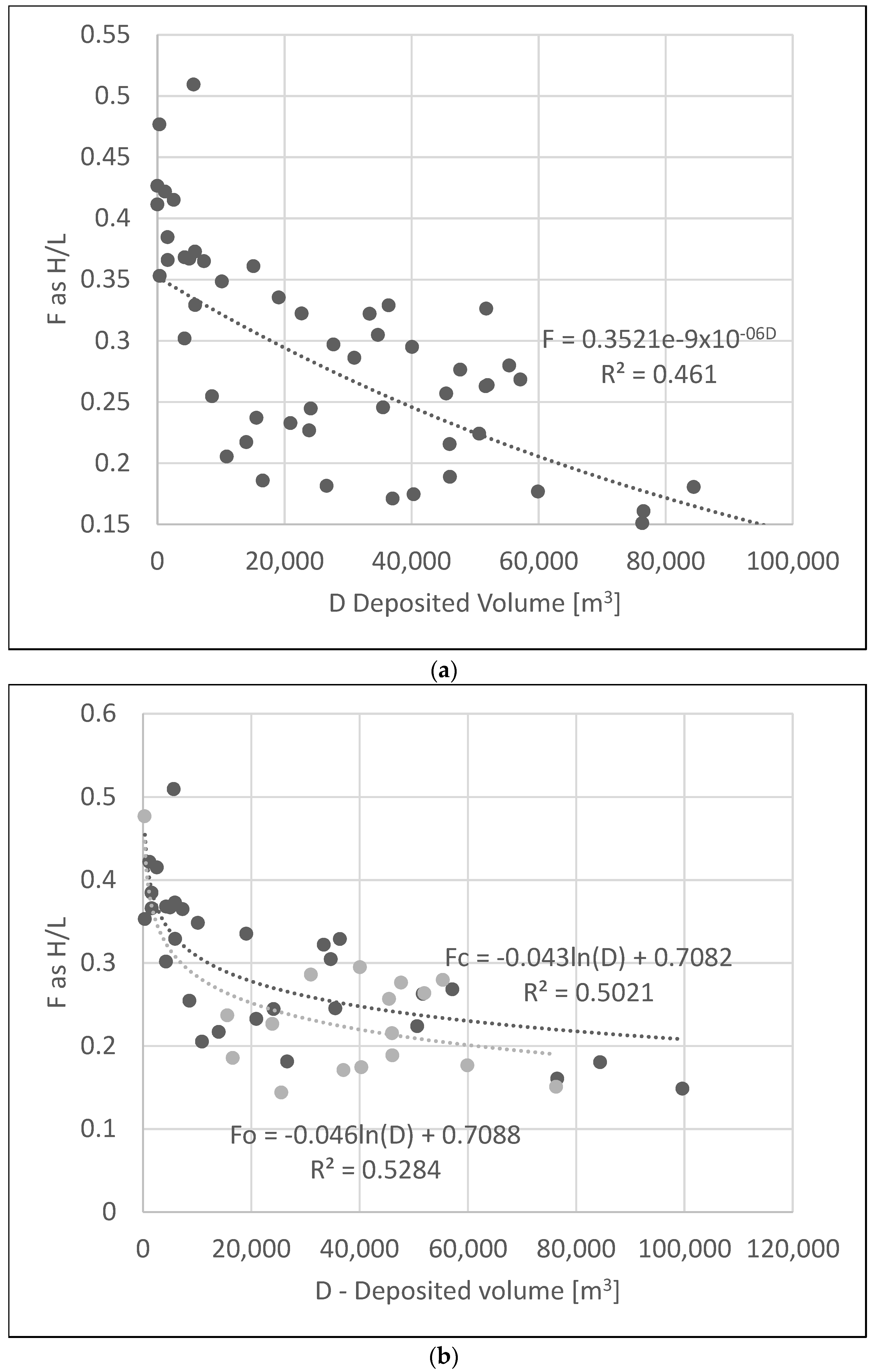
3.3. The Fahrböschung for “Open-Slopes” and “Valley-Confined” Flows

For the sampled population, the Fahrböschung is comprised between 0.15 and 0.55 +/− ~5% (allowing three outliers, i.e., 5% of the dataset), and it decreases as the volume of the deposit increases. The smallest mass movements < 4000 m³ have a Fahrböschung of >0.3, while the mass movements with a volume >59,000 m³ are all below 0.2. Those to end member groups link through a constantly decreasing F as V increases, following a relationship (Figure 7a), as follows:

$$\mathrm{F}={0.3521}^{-9\ast {10}^{-06}\mathrm{D}}$$

(13)

Separating the two types of mass movements (valley-confined and open-slope), there is once again no clear distinction between the two types of movements and they seem to have relatively similar mobility (Figure 7b), as represented by the two relation equations (Equations (14) and (15)):

F_c = −0.043ln(D) + 0.7082

(14)

F_o = −0.046ln(D) + 0.7088

(15)

As the Fahrböschung is a proxy of the mobility of the landslides, one author hypothesized that it should have a linear effect on how the material spreads. Comparing the ratio of width per length of the deposit (W/LD), this ratio SF was computed against F (Figure 8). There is no strong linear correlation between the two datasets, because of a seemingly unvarying Fahrböschung set of data F < 0.1. However, an envelope with a positive trends appears, with the mass-movements that have the lowest-mobility being the movements that tend to spread the most (Figure 8).

4. Discussion

4.1. Result Summary

The mass-movements measured from LiDAR and aerial photographs’ remote sensing are relatively homogeneous in term of the deposits’ geometry, following the relation LD = 2.2492 W^1.0296 with a R² = 0.8985. If one considers this geometric relation to be the result of mass movements ending on a sub-horizontal surface, it is then possible to compare these results with the deposits of mass movements that have stopped on counter-slopes in order to investigate the role of the latter, for instance. The k-parameter follows a k = 2.1842ln(S) − 10.167 relation with the surface area of the deposit, with variations depending on whether the deposit was created by an open-slope or a valley-controlled landslide (Equations (13) and (14)). The T parameter was more spread and could not lead to any significant relation without the construction of an empirical ceiling-function. The T equation divided the total volume of the deposit by the surface area of the deposit to the power 2/3, multiplied by the tangent of the slope deposit (Equation (9)). For the sake of the discussion this can be simplified by reducing it to a 2D cross section, so that T_2D is (Equation (16)):

$${\mathrm{T}}_{2\mathrm{D}}\approx \frac{\mathrm{A}}{\mathrm{Z}/\mathrm{LD}}$$

(16)

where A is a longitudinal cross-section area of the deposit, and Z and LD are the deposit height and LD the length of the deposit (cf. Figure 2). In other words, the cross section A is controlled by the maximum height difference between the highest and the lowest topographic point of the deposit. This value is also an expression of the effective stress of the deposited soil, according to Terzaghi’s principle (Equation (17)):

$${\mathsf{\sigma }}^{\prime }=\mathsf{\sigma }-\mathrm{u}$$

(17)

where σ’ is the effective stress, σ is the total stress and u is the pore pressure.

Takahashi (2014) found, from experiments, that T was 5/12 for debris-flows, which is lower than the ceiling value T = −0.0001S + 3.75. If we discard the small variability as a function of S, 3.75 is more than nine times higher than the values of the laboratory debris-flow. Consequently, starting from Terzaghi’s principle, the high T values found in this study signify that the water pore pressure has less influence on the deposit and, thus, during transport, the material moves with less water than it would in a rain-triggered debris-flow. For Quaternary studies, when only the deposit remains, it should therefore be possible to identify the process as either a seismic-driven or water-driven debris-flow, if it is possible to retrieve the T value. However, the dataset also shows an important variability, and T values close to those proposed by Takahashi (2014) were also recorded, suggesting that some of the mass movements observed eventually had more water available or were further liquefied by secondary processes.

The Fahrböschung followed a typical pattern, with the larger deposit-volumes displaying a F inferior to the ones of smaller landslides; the deposits generated from valley-confined movements yielded a Fahrböschung of Fc = −0.043ln(D) + 0.7082 with an R² = 0.5021, while the open-slopes’ movements displayed a Fo = −0.046ln(D) + 0.7088 with R² = 0.5284.

4.2. The Hokkaido Iburi-Tobu Earthquake Landslides Were Extremely Mobile

The Fahrböschung, whether it is expressed as an angle or as a ratio height to length, is a useful comparator of the mobility of mass movements. It has been shown to decrease with the mass and the volume of mass movements, even for types other than the debris-flow types encountered in the present study. At the Naga landslide, for instance, Lagmay et al. [37] calculated a Fahrböschung (as H/L) of 0.17 (or 9 degrees), while Catane et al. [38] calculated 0.16 (or 9 degrees), for estimated volumes of 11 and 27 million cubic meters, respectively. At the Guinsaugon landslide (February 2006, Leyte Island, Philippines), authors have calculated the H/L to be 0.17 to 0.21 [37], with, in both cases, volumes of 15 million cubic meters. On 23 September 1991, the rock avalanche of Zhaotong (China) travelled 3650 m horizontally for a vertical drop of 960 m, resulting in a Fahrböschung of 14.7 degrees or 0.263 expressed as H/L [39]. If we use the relation obtained in the present study between H/L and V (as H/L = 0.046ln(V) + 0.7088), the present formula is much lower than values calculated at other sites (it gives, for instance, 0.028 for the 27 million cubic meter Naga landslide, instead of the measured 0.16).

This suggests that the Iburi-Tobu Hokkaido earthquake landslides were extremely mobile compared to other values found in the literature. Direct comparisons of different landslides is, however, arduous, because of the variety of flowing processes, materials and grain-size. For granular flow, for instance, Coombs et al. [40] have shown that the Fahrböschung decreased by 14% from 25 to 21.4 degrees when the mean grain sizes in the experiments changed from 3 to 25 mm. Besides the original grain-size effects, the self-comminution of the grains impacts stability and shear strength [41], as does the presence of volcanic material in soils. This has been shown in other locations in Japan [42]. This work found that the dry density could be as low as 13 to kN/m³, values that are comparable to the 10 to 15 kN/m³ found in Tenerife [43] or 11 to 14 kN/m³ for the Cangahua volcanic soil formation in South America [44].

Because of the variability of the parameters at play, the authors reduced the sum of these issues to the Mohr-Coulomb effective stress theory in order to discuss the high-mobility of the Hokkaido Iburi-Tobu co-seismic landslides from a practical perspective. In its simplest form, the Mohr-Coulomb failure criterion can be expressed as:

$${\mathsf{\tau }}_{\mathrm{f}}= {\mathrm{C}}^{\prime }+{\left({\mathsf{\sigma }}_{\mathrm{f}}-{\mathrm{u}}_{\mathrm{w}}\right)}_{\mathrm{f}}\tan {\mathsf{\phi }}^{\prime }$$

(18)

where the term on the left is the maximum stress a soil allows before failing, the first term on the right side of the equation is the cohesion, and the second term is the effective stress multiplied by the tangent of the angle of friction. This equation can be used to describe the state of a material on a slope, but a non-linear envelope is needed to take into account the seismic loading [45] and is expressed with a linear coefficient [46], as follow:

$$\mathsf{\tau }={\mathrm{C}}_0\ast {\left(1+\frac{{\mathsf{\sigma }}_{\mathrm{n}}}{{\mathsf{\sigma }}_1}\right)}^{1/\mathrm{m}}$$

(19)

where, is the shear stress ${\mathsf{\sigma }}_{\mathrm{n}}$ is the normal stress, ${\mathsf{\sigma }}_1$ is the intercept of the envelope shear stress with the normal stress axis [46], ${\mathrm{C}}_0$ is the cohesion, and 1/m is the non-linear parameter. Because the present contribution is a remote sensing contribution, and not a geotechnical analysis, the goal is not to solve these equations, but to compare the two in order to reflect the unusually long runout and low H/L, even in cases where the landslide volumes were small.

From Equation (19), when m is more or equal to 1, the Mohr-Coulomb envelope is therefore rising at a lower rate than the linear Mohr-Coulomb envelope, so that for a similar slope the normal stress that the slope can sustain before failing is lower under seismic activity.

By this process, the authors would argue that there may be a reduction of the “local effects” explaining the relative homogeneity in the shapes of the landslides (cf. Equation (11) with a R² = 0.89). This effect needs further evidence and investigation, but a potential research direction certainly includes the role of the shaking during the movement, limiting deposition due to local effects, and also the homogeneous start of the mass movements. As rainfall will fall on one catchment more than another, heterogeneity in the mass movements may arise. Finally, the factor of the safety of each slope may become irrelevant when considering the threshold, as intense surface acceleration may produce energy which throws all the slopes way above their factor of safety threshold. This would then homogenize the mass-movements, limiting local factors.

Finally, effective remote sensing needs to be combined with spatially-dense data on the material shear strength to complete the high-resolution topographic dataset that has emerged in recent years.

5. Conclusions

High-Resolution Topographic data combined with remotely-sensed imagery has been shown to be an effective tool in generating sets of descriptive parameters of landslide deposits. The relationship between the width and length of the deposit has shown good correlations, suggesting that the conditions of lateral spreading during deposition are relatively similar. This differs from rain-triggered landslides, because the internal friction and cohesion can vary across a broad range. In the present case, however, the surface acceleration has contributed to homogenizing them. Arguably, this process contributed towards the convergence of planform indicators. In contrast, the T parameter developed for debris-flow has shown a weak correlation with the parameters of shape and volume. This weak correlation was interpreted as being the eventual effect of continuous excitation by the earthquake. The T-indicator is an indicator of the energy balance between potential energy and its dissipation during movement. Therefore, the seismic dissipation has certainly disrupted the result of this indicator.

Although it is a negative result, this means that the T-factor can be used in forensic geosciences to assess whether a landslide moved due to a rainfall-trigger or due to a seismic excitation.

The present research has shown the exceptional mobility of landslides, and that one research direction that spans beyond the realm of remote sensing is the field investigation of potential influences on volcanic fallout, as this is often the case in Japan. We would further argue that increasingly the amount of “tele-connections” between landforms and soil formation is certainly a step that is necessary; just as these have been shown to play a potential role in linking tsunamis and mountain debris flows through atmospheric tele-connections [47].

References

1. Cheung, R.W.M. Landslide risk management in Hong Kong. Landslides 2021, 1–17. [Google Scholar] [CrossRef]
2. Wong, H.N.; Ko, F.W.Y. Landslide risk assessment—Application and Practice. In Geo-Report 195; The Government of Hong Kong Special Administration Region: Hongkong, China, 2006; 279p. [Google Scholar]
3. Gao, L.; Zhang, L.M.; Cheung, R.W.M. Relationships between natural terrain landslide magnitudes and triggering rainfall based on a large landslide inventory in Hong Kong. Landslides 2017, 15, 727–740. [Google Scholar] [CrossRef]
4. Osanai, N.; Yamada, T.; Hayashi, S.; Katsura, S.; Furuichi, T.; Yanai, S.; Murakami, Y.; Miyazaki, T.; Tanioka, Y.; Takiguchi, S.; et al. Characteristics of landslides caused by the 2018 Hokkaido Eastern Iburi Earthquake. Landslides 2019, 16, 1517–1528. [Google Scholar] [CrossRef]
5. Zhao, B.; Wang, Y.; Feng, Q.; Guo, F.; Zhao, X.; Ji, F.; Liu, J.; Ming, W. Preliminary analysis of some characteristics of coseismic landslides induced by the Hokkaido Iburi-Tobu earthquake (5 September 2018). Catena 2020, 189, 104502. [Google Scholar] [CrossRef]
6. Ohzono, M.; Takahashi, R.; Ito, C. Spatiotemporal crustal strain distribution around the Ishikari-Teichi-Toen fault zone estimated from global navigation satellite system data. Earth Planets Space 2019, 71, 50. [Google Scholar] [CrossRef]
7. Kobayashi, T.; Hayashi, K.; Yarai, H. Geodetically estimated location and geometry of the fault plane involved in the 2018 Hokkaido Eastern Iburi earthquake. Earth Planets Space 2019, 71, 62. [Google Scholar] [CrossRef]
8. Kubo, H.; Iwaki, A.; Suzuki, W.; Aoi, S.; Sekiguchi, H. Estimation of the source process and forward simulation of long-period ground motion of the 2018 Hokkaido Eastern Iburi, Japan, earthquake. Earth Planets Space 2020, 72, 20. [Google Scholar] [CrossRef] [Green Version]
9. Takai, N.; Shigefuji, M.; Horita, J.; Nomoto, S.; Maeda, T.; Ichiyanagi, M.; Takahashi, H.; Yamanaka, H.; Chimoto, K.; Tsuno, S.; et al. Cause of destructive strong ground motion within 1–2 s in Mukawa town during the 2018 Mw 66 Hokkaido eastern Iburi earthquake. Earth Planets Space 2019, 71, 67. [Google Scholar] [CrossRef] [Green Version]
10. Yamagishi, H.; Yamazaki, F. Landslides by the 2018 Hokkaido Iburi-tobu earthquake on setpember 6. Landslides 2018, 15, 2521–2524. [Google Scholar] [CrossRef] [Green Version]
11. Chang, M.; Zhou, Y.; Zhou, C.; Hales, T.C. Coseismic landslides induced by the 2018 Mw 6.6 Iburi, Japan, Earthquake: Spatial distribution, key factors weight and susceptibility regionalization. Landslides 2021, 18, 755–772. [Google Scholar] [CrossRef]
12. Tsai, T.-T.; Tsai, K.-J.; Shieh, C.-L. Large Scale Landslide Database System Established for the Reservoirs in Southern Taiwan. In Proceedings of the 19th EGU General Assembly, Vienna, Austria, 23–28 April 2017; p. 13505. [Google Scholar]
13. Calista, M.; Miccadei, E.; Piacentini, T.; Sciarra, N. Morphostructural, Meteorological and Seismic Factors Controlling Landlsides in Weak Rocks: The Case Studies of Castelnuovo and Ponzano (North East Abruzzo, Central Italy). J. Geosci. 2019, 9, 122. [Google Scholar] [CrossRef] [Green Version]
14. Pu, X.; Wan, L.; Wang, P. Initiation mechanism of mudflow-like loess landslide induced by the combined effect of earthquakes and rainfall. Nat. Hazards 2021, 105, 3079–3097. [Google Scholar] [CrossRef]
15. Morelli, S.; Prazzi, V.; Frodella, W.; Fanti, R. Kinematic Reconstruction of a Deep-Seated Gravitational Slope Deformation by Geomophic Analyses. J. Geosci. 2018, 8, 26. [Google Scholar] [CrossRef] [Green Version]
16. Agliardi, F.; Crosta, G.B.; Zanchi, A. Strutural constraints on deep-seated slope deformation kinematics. Eng. Geol. 2001, 59, 83–102. [Google Scholar] [CrossRef]
17. Bovenga, F.; Nutricato, R.; Refice, A.; Wasowski, J. Application of multi-temporal differential interferometry to slope instability detection in urban/peri-urban areas. Eng. Geol. 2006, 88, 219–240. [Google Scholar] [CrossRef]
18. Tomas, R.; Li, Z.; Lopez-Sanchez, J.M.; Liu, P.; Singleton, A. Using wavelet tools to analyse seasonal variations from InSAR time-series data: A case study of the Huangtupo landslide. Landslides 2016, 13, 437–450. [Google Scholar] [CrossRef] [Green Version]
19. Gomez, C.; Allouis, T.; Lissak, C.; Hotta, N.; Shinohara, Y.; Hadmoko, D.S.; Vilimek, V.; Wassmer, P.; Lavigne, F.; Setiawan, A.; et al. High-resolution Point-Cloud for Landslides in the 21st Century: From Data Acquisition to New Processing Concepts. In Understanding and Reducing Landslide Disaster Risk, ICL Contribution to Landslide Disaster Risk Reduction; Arbanas, Ž., Bobrowsky, P.T., Konagai, K., Sassa, K., Takara, K., Eds.; Springer: Cham, Switzerland, 2021; pp. 199–213. [Google Scholar]
20. Strozzi, T.; Ambrosi, C. SAR Interferometric Point Target Analysis and Interpretation of Aerial Photographs for Landslides Investigations in Ticino, southern Switzerland. In Proceedings of the ENVISAT Symposium, Montreux, Switzerland, 23–27 April 2007. [Google Scholar]
21. Gomez, C.; Hayakawa, Y.; Obanawa, H. A study of Japanese landscapes using structure from motion derived DSMs and DEMs based on historical aerial photographs: New opportunities for vegetation monitoring and diachronic geomorphology. Geomorphology 2015, 242, 11–20. [Google Scholar] [CrossRef] [Green Version]
22. Koukouvelas, I.K.; Nikolakopoulos, K.G.; Zygouri, V.; Kyriou, A. Post-seismic monitoring of cliff mass wasting using an unmanned aerial vehicle and field data at Egremni, Lefkada Island, Greece. Geomorphology 2020, 367, 107306. [Google Scholar] [CrossRef]
23. Clapuyt, F.; Vanacher, V.; Oost, K.V. Reproducibility of UAV-based earth topography reconstructions based on Structure-from-Motion algorithms. Geomoprhology 2016, 260, 4–15. [Google Scholar] [CrossRef]
24. Mateos, R.M.; Azanon, J.M.; Roldan, F.J.; Notti, D.; Perez-Pena, V.; Galve, J.P.; Perez-Garcia, J.L.; Colomo, C.M.; Gomez-Lopez, J.M.; Montserrat, O.; et al. The combined use of PSInSAR and UAV photogrammetry techniques for the analysis of the kinematics of a coastal landslide affecting an urban area (SE Spain). Landslides 2017, 14, 743–754. [Google Scholar] [CrossRef]
25. Peternal, T.; Kuemlj, S.; Ostir, K.; Komac, M. Monitoring the Potoska planina landslide (NW Slovenia) using UAV photogrammetry and tachymetric measurements. Landslides 2017, 14, 395–406. [Google Scholar] [CrossRef]
26. Eker, R.; Aydin, A.; Hubl, J. Unmanned aerial vehicle (UAV)-based monitoring of a landslide: Gallenzerkogel landslide (Ybbs-Lower Austria) case study. Environ. Monit Assess. 2018, 190, 1–14. [Google Scholar] [CrossRef]
27. Garcia-Pena, R.; Alcantara-Ayala, I. The use of UAVs for landslide disaster risk research and disaster risk management: A literature review. J. Mt. Sci. 2021, 18, 482–498. [Google Scholar] [CrossRef]
28. Litoseliti, A.; Koukouvelas, I.K.; Nikolakopoulos, G.; Zygouri, V. An Event-Based Inventory Approach in Landslide Hazard Assessment: The Case of the Skolis Mountain, Northwest Peloponnese, Greece. ISPRS Int. J. Geo-Inf. 2020, 9, 457. [Google Scholar] [CrossRef]
29. Hungr, O. Classification and terminology. In Debris-Flow Hazards and Related Phenomena; Jakob, M., Hungr, O., Eds.; Springer: Berlin/Heidelberg, Germany, 2005; pp. 9–24. [Google Scholar]
30. Scheidl, C.; Rickenmann, D. Empirical prediction of debris-flow mobility and deposition on fans. Earth Surf. Process. Landf. 2010, 35, 157–173. [Google Scholar] [CrossRef]
31. Crosta, G.B.; Cucchiaro, S.; Frattini, P. Validation of semi-empirical relationships for the definition of debris-flow behavior in granular materials. In Debris-Flow Hazards Mitigation; Chen, C.L., Major, J.J., Eds.; Mill Press: Rotterdam, The Netherlands, 2003; pp. 821–831. [Google Scholar]
32. Iverson, R.M.; Schilling, S.P.; Vallance, J.W. Objective delineation of lahar-inundation hazard zones. Geol. Soc. Am. Bull. 1998, 110, 972–984. [Google Scholar] [CrossRef]
33. Corominas, J. The angle of reach as a mobility index for small and large landslides. Can. Geotech. J. 1996, 33, 260–271. [Google Scholar] [CrossRef]
34. Rickenmann, D. Runout prediction methods. In Debris-Flow Hazards and Related Phenomena; Jakob, M., Hungr, O., Eds.; Springer: Berlin/Heidelberg, Germany, 2005; pp. 305–324. [Google Scholar]
35. Rickenmann, D. Empirical relationships for debris flows. Nat. Hazards 1999, 19, 47–77. [Google Scholar] [CrossRef]
36. Takahashi, T. Debris Flow—Mechanics, Prediction and Countermeasures, 2nd ed.; CRC Press/Balkema: Boca Raton, FL, USA, 2014; 540p. [Google Scholar]
37. Lagmay, A.M.F.; Escape, C.M.; Ybanez, A.A.; Suarez, J.K.; Cuaresma, G. Anatomy of the Naga City Landslide and Comparison with Historical Debris Avalanches and Analog Models. Front. Earth Sci. 2020, 8, 312. [Google Scholar] [CrossRef]
38. Catane, S.; Veracruz, N.; Flora, J.; Go, C.; Enrera, R.; Santos, E. Mechanism of a low-angle translational block slide: Evidence from the September 2018 Naga landslide, Philippines. Landslides 2019, 16, 1709–1719. [Google Scholar] [CrossRef]
39. Xing, A.; Wang, G.; Yin, Y.; Tang, C.; Xu, Z.; Li, W. Investigation and dynamic analysis of a catastrophic rock avalanche on September 23, 1991, Zhaotong, China. Landslides 2016, 13, 1035–1047. [Google Scholar] [CrossRef]
40. Coombs, S.P.; Apostolov, A.; Take, W.A.; Benoit, J. Mobility of dry granular flows of varying collisional activity quantified by smart rock sensros. Can. Geotech. J. 2020, 57, 1484–1496. [Google Scholar] [CrossRef]
41. Gomez, C.; Shinohara, Y.; Hotta, N.; Tsunetaka, H. In-flow Self-comminution of Debris-flow and Lahars: Fragmentation and Grinding Experiments for the Dacites from Unzen-Volcano. In Proceedings of the 10th Symposium of Sediment Hazards, Japan, 9 September 2020; pp. 127–132. [Google Scholar]
42. Yamanouchi, T.; Murata, H. Brittle failure of a volcanic ash soil “Shirasu”. In Proceedings of the 8th International Conference on Soil Mechanics and Foundation Engineering, Moscow, Russia, 6–11 August 1973; Volume 1, pp. 495–500. [Google Scholar]
43. Gonzalez de Vallejo, L.I.; Jimenez Salas, J.A.; Leguey Jiminez, S. Engineering geology of the tropical volcanic soils of La Laguna, Tenerife. Eng. Geol. 1981, 17, 1–17. [Google Scholar] [CrossRef]
44. O’Rourke, T.D.; Crespo, E. Cemented volcanic soil. J. Geotech. 1988, 114, 1126–1147. [Google Scholar] [CrossRef]
45. Zhang, X.J.; Chen, W.F. Stability analysis of slopes with general nonlinear failure criterion. Int. J. Numer. Anal. Methods Geomech. 1987, 11, 33–50. [Google Scholar] [CrossRef]
46. Zhao, L.-H.; Cheng, X.; Dan, H.-C.; Tang, Z.-P.; Zhang, Y. Effect of the vertical earthquake component on permanent seismic displacement of soil slopes based on the nonlinear Mohr-Coulomb failure criterion. Soils Founds 2017, 57, 237–251. [Google Scholar] [CrossRef]
47. Gomez, C.; Soltanzadeh, I. Boundary crossing and non-linear theory in earth-system sciences—A proof of concept based on tsunami and post-eruption scenarios on Java Island, Indonesia. Earth Surf. Process Landf. 2012, 37, 790–796. [Google Scholar] [CrossRef]
Figure 1. The Hokkaido Iburi-Tobu Earthquake of 2018. (1) Map of Japan indicating the position of Hokkaido island and prefecture; (2) Research location in the Southern Part of Hokkaido; (3) Location of the epicenter symbolized by a red start and the digitized mass movements in yellow. The locations of photographs 4 and 5 are also provided. (4) Landslide mixing sediments and wood debris that stopped on a pseudo-horizontal valley floor—the object of the study. (5) Mass movements with mixed deposits on slopes and constrained within narrow valleys—not used in the present study.
Remotesensing 13 03421 g001
Figure 2. The basic linear parameters used to calculate the geometric data and the empirical factors (L: maximum horizontal distance travelled by the mass-movement; W: maximum width of the deposit; LD: maximum horizontal length of the deposit pass the slope break; Ht: Maximum elevation at the scarp the landslide started from; Hb: Minimum elevation at the toe of the deposit; H: Difference of Hb subtracted from Ht; Z: the maximum height of the deposit, used to calculate the slope of the deposit’s surface; B: the elevation of the underlying topography at the slope break and at the toe of the deposit).
Remotesensing 13 03421 g002
Figure 3. Relation between the width of the deposits and the length of the deposits for all the samples that stopped on pseudo-horizontal valley floor.
Remotesensing 13 03421 g003
Figure 4. Relation between the power-relation scalar k (Equation (10)) and the surface of the deposits (the reader will note the apparent existence of two curves, but the origin of those could not be determined using remote sensing data only).
Remotesensing 13 03421 g004
Figure 5. Relation between the power-relation scalar k (Equation (10)) and the surface of the deposits, separating the open-slope landslides (dark grey triangles) and the valley-confined landslides (light grey circles). The subscripts “o” and “c” refer to the open-slope and the confined landslides.
Remotesensing 13 03421 g005
Figure 6. The relation between the Surface area and the T scalar relating the volume to the area and the slope gradient of the deposit, allowing for ~5% outliers. The intermittent line is the equation of the ceiling values T = −0.0001 S + 3.75.
Remotesensing 13 03421 g006
Figure 7. (a) The Fahrböschung F is calculated against the volume of the deposits for the selected landslides. (b) Relation between the deposited volumes and the Fahrböschung (F) separating the deposits from valley-confined mass-movements (Fc) and the deposits resulting from open-slope mass-movements (Fo). Both display comparatively similar Fahrböschung relations.
Remotesensing 13 03421 g007
Figure 8. The Fahrböschung F as a function of SF, being the ratio of the width to the length of the deposit, showing its ability to spread laterally.
Remotesensing 13 03421 g008
Publisher’s Note: MDPI stays neutral with regard to jurisdictional claims in published maps and institutional affiliations.