
Drone-Assisted Confined Space Inspection and Stockpile Volume Estimation

 , , , and
Abstract
:
1. Introduction
2. Research Background
2.1. Examples of Drone Missions in Confined Spaces
2.2. Challenges of Flying Drones in Confined Spaces
2.3. Commercial off-the-Shelf Indoor Inspection and Mapping Drones
2.4. Outdoor Aerial Stockpile Volume Estimation
2.5. Dust Effects on LiDAR Sensors
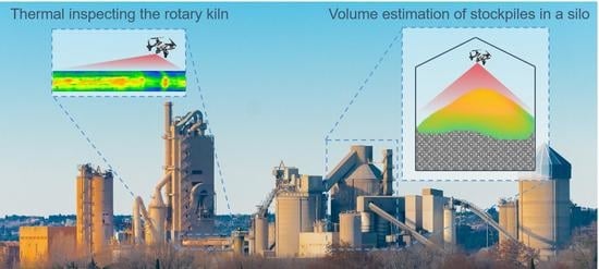
3. Current Health and Safety Challenges in Cement Plants
3.1. Overview
3.2. Revisiting Confined Space Safety Challenges

| Country/ Region | Period | Incidents | Fatalities | Fatality Rate per 100,000 Workers | Source |
|---|---|---|---|---|---|
| Australia | 2000–2012 | 45 | 59 | 0.05 | [65] |
| New Zealand | 2007–2012 | 4 | 6 | 0.05 | [54] |
| Singapore | 2007–2014 | N/A | 18 | 0.08 | [54] |
| Quebec, Canada | 1998–2011 | 31 | 41 | 0.07 | [50] |
| British Columbia, Canada | 2001–2010 | 8 | 17 | N/A | [54] |
| USA | 1980–1989 | 585 | 670 | 0.08 | [66] |
| USA | 1997–2001 | 458 | 0.07 | [67] | |
| USA | 1992–2005 | 431 | 530 | 0.03 | [68] |
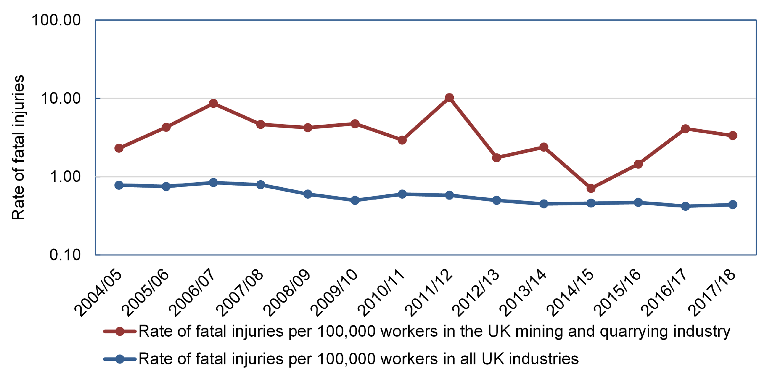
| UK and Ireland | N/A | N/A | 15–25/year | 0.05 | [69,70] |
| Italy | 2001–2015 | 20 | 51 | N/A | [71] |
| Jamaica | 2005–2017 | 11 | 17 | N/A | [71] |
3.3. Indoor Stockpile Volume Estimation
3.4. Drones Safety Regulations
4. Proposed Drone-Assisted Solution for Stockpile Volume Estimation
4.1. Overview
4.2. Simulation Framework
4.2.1. Simulation Setup and Selection of Sensors
4.2.2. Indoor Localisation System
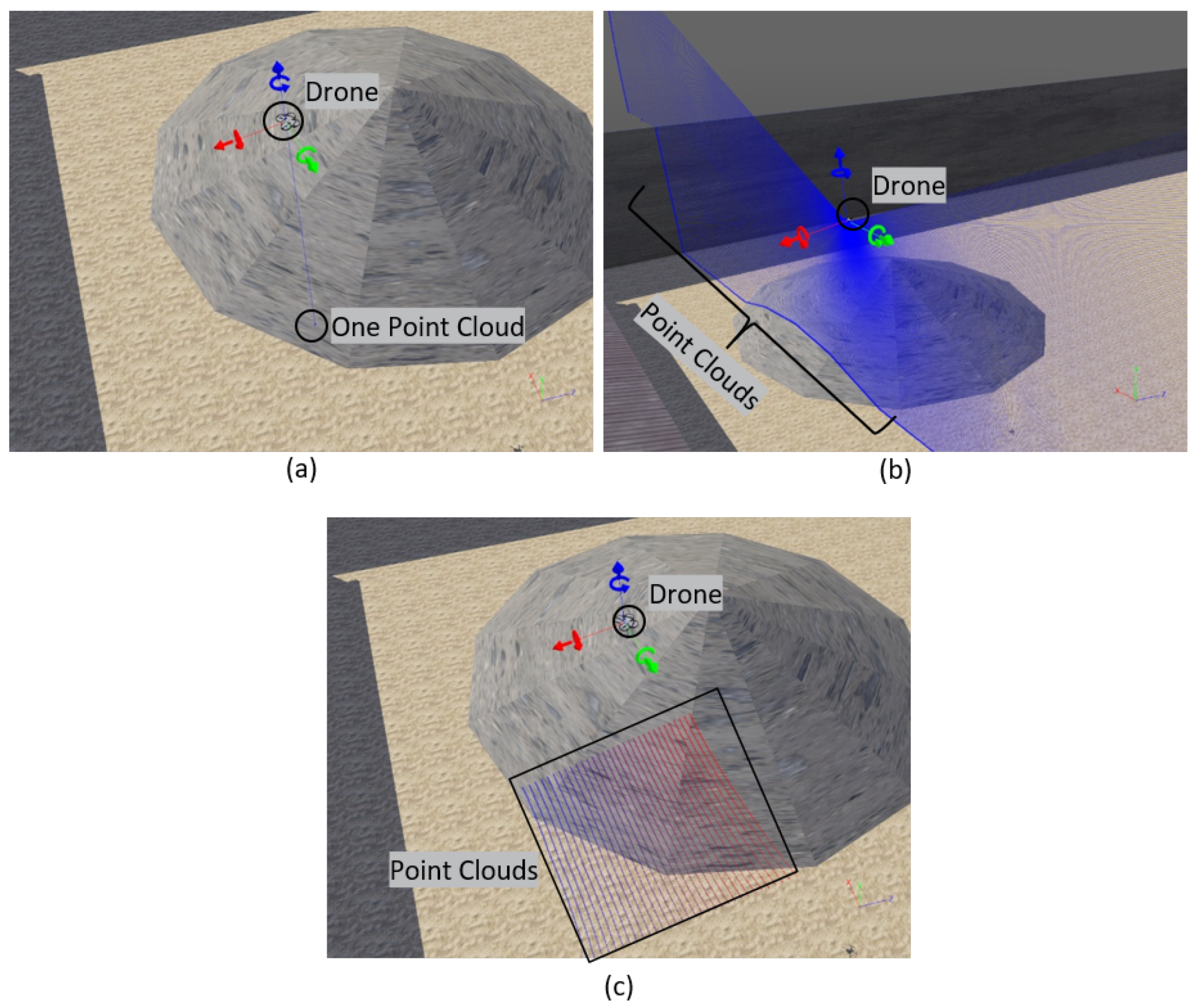
4.2.3. Locating and Filtering Point Clouds
4.2.4. Surface Generation
4.2.5. Mission Design
4.2.6. Simulation Results and Discussions
4.2.7. Stockpile Volume Estimation Using 3D Static Scanners
4.3. Industrial Case Study
4.3.1. Instrumentation
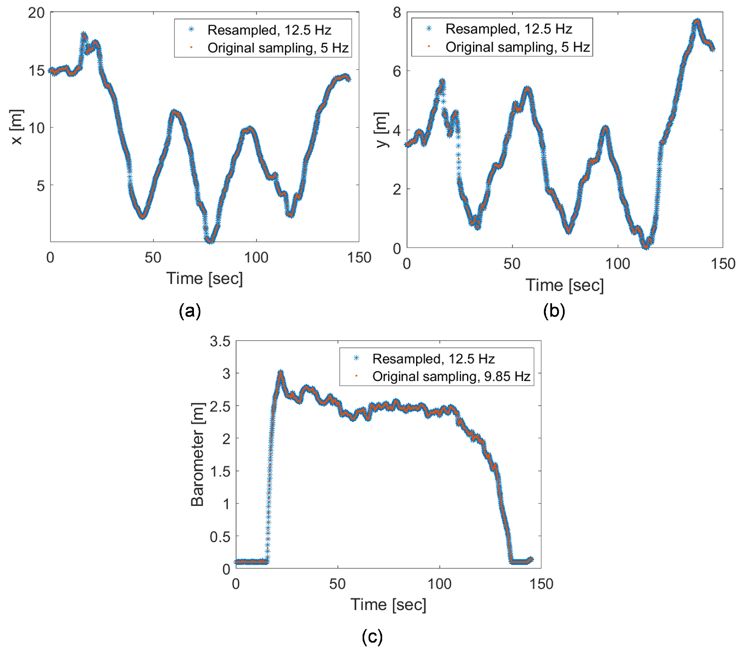
4.3.2. Data Collection and Processing
4.3.3. Results from Flight Tests
5. Cost-Benefit Analysis
6. Concluding Remarks and Future Work
Author Contributions
Funding
Institutional Review Board Statement
Informed Consent Statement
Data Availability Statement
Acknowledgments
Conflicts of Interest
References
- Siebert, S.; Teizer, J. Mobile 3D mapping for surveying earthwork projects using an Unmanned Aerial Vehicle (UAV) system. Autom. Constr. 2014, 41, 1–14. [Google Scholar] [CrossRef]
- Otto, A.; Agatz, N.; Campbell, J.; Golden, B.; Pesch, E. Optimization approaches for civil applications of unmanned aerial vehicles (UAVs) or aerial drones: A survey. Networks 2018, 72, 411–458. [Google Scholar] [CrossRef]
- Liu, D.; Chen, J.; Hu, D.; Zhang, Z. Dynamic BIM–augmented UAV safety inspection for water diversion project. Comput. Ind. 2019, 108, 163–177. [Google Scholar] [CrossRef]
- Miranda, J.; Ponce, P.; Molina, A.; Wright, P. Sensing, smart and sustainable technologies for Agri-Food 4.0. Comput. Ind. 2019, 108, 21–36. [Google Scholar] [CrossRef]
- Nabawy, M.R.A.; ElNomrossy, M.M.; Abdelrahman, M.M.; ElBayoumi, G.M. Aerodynamic shape optimisation, wind tunnel measurements and CFD analysis of a MAV wing. Aeronaut. J. 2012, 116, 685–708. [Google Scholar] [CrossRef] [Green Version]
- Ahmed, M.R.; Abdelrahman, M.M.; ElBayoumi, G.M.; ElNomrossy, M.M. Optimal wing twist distribution for roll control of MAVs. Aeronaut. J. 2011, 115, 641–649. [Google Scholar] [CrossRef]
- Shearwood, T.R.; Nabawy, M.R.A.; Crowther, W.J.; Warsop, C. A Novel Control Allocation Method for Yaw Control of Tailless Aircraft. Aerospace 2020, 7, 150. [Google Scholar] [CrossRef]
- Shearwood, T.R.; Nabawy, M.R.; Crowther, W.; Warsop, C. A Control Allocation Method to Reduce Roll-Yaw coupling on Tailless Aircraft. In Proceedings of the AIAA Scitech 2021 Forum, Virtual Event, 11–15, 19–21 January 2021. [Google Scholar] [CrossRef]
- Health and Safety Statistics. Available online: https://www.hse.gov.uk/statistics (accessed on 12 July 2020).
- SAFTENG. Available online: http://www.safteng.net (accessed on 1 June 2020).
- Kas, K.A.; Johnson, G.K. Using unmanned aerial vehicles and robotics in hazardous locations safely. Process. Saf. Prog. 2020, 39, 1–13. [Google Scholar] [CrossRef]
- Esfahlani, S.S. Mixed reality and remote sensing application of unmanned aerial vehicle in fire and smoke detection. J. Ind. Inf. Integr. 2019, 15, 42–49. [Google Scholar] [CrossRef]
- Anderson, M.J.; Sullivan, J.G.; Talley, J.L.; Brink, K.M.; Fuller, S.B.; Daniel, T.L. The “Smellicopter,” a bio-hybrid odor localizing nano air vehicle. In Proceedings of the 2019 IEEE/RSJ International Conference on Intelligent Robots and Systems (IROS), Macao, China, 3–8 November 2019; pp. 6077–6082. [Google Scholar]
- Lee, S.; Har, D.; Kum, D. Drone-assisted disaster management: Finding victims via infrared camera and lidar sensor fusion. In Proceedings of the 2016 3rd IEEE Asia-Pacific World Congress on Computer Science and Engineering (APWC on CSE), Nadi, Fiji, 4–6 December 2016; pp. 84–89. [Google Scholar]
- Burgués, J.; Hernández, V.; Lilienthal, A.; Marco, S. Smelling Nano Aerial Vehicle for Gas Source Localization and Mapping. Sensors 2019, 19, 478. [Google Scholar] [CrossRef] [Green Version]
- Turner, R.M.; MacLaughlin, M.M.; Iverson, S.R. Identifying and mapping potentially adverse discontinuities in underground excavations using thermal and multispectral UAV imagery. Eng. Geol. 2020, 266, 105470. [Google Scholar] [CrossRef]
- Papachristos, C.; Khattak, S.; Mascarich, F.; Dang, T.; Alexis, K. Autonomous Aerial Robotic Exploration of Subterranean Environments relying on Morphology–aware Path Planning. In Proceedings of the 2019 IEEE International Conference on Unmanned Aircraft Systems (ICUAS), Atlanta, GA, USA, 11–14 June 2019; pp. 299–305. [Google Scholar]
- Castaño, A.R.; Romero, H.; Capitán, J.; Andrade, J.L.; Ollero, A. Development of a Semi-autonomous Aerial Vehicle for Sewerage Inspection. In Robot 2019: Fourth Iberian Robotics Conference; Silva, M.F., Luís Lima, J., Reis, L.P., Sanfeliu, A., Tardioli, D., Eds.; Springer International Publishing: Cham, Switzerland, 2020; pp. 75–86. [Google Scholar]
- Ajay Kumar, G.; Patil, A.K.; Patil, R.; Park, S.S.; Chai, Y.H. A LiDAR and IMU Integrated Indoor Navigation System for UAVs and Its Application in Real-Time Pipeline Classification. Sensors 2017, 17, 1268. [Google Scholar] [CrossRef] [Green Version]
- Cook, Z.; Kazemeini, M.; Barzilov, A.; Yim, W. Low-altitude contour mapping of radiation fields using UAS swarm. Intell. Serv. Robot. 2019, 12, 219–230. [Google Scholar] [CrossRef]
- Hennage, D.H.; Nopola, J.R.; Haugen, B.D. Fully autonomous drone for underground use. In Proceedings of the 53rd U.S. Rock Mechanics/Geomechanics Symposium. American Rock Mechanics Association, New York, NY, USA, 23–26 June 2019. [Google Scholar]
- De Croon, G.; De Wagter, C. Challenges of Autonomous Flight in Indoor Environments. In Proceedings of the 2018 IEEE/RSJ International Conference on Intelligent Robots and Systems (IROS), Madrid, Spain, 1–5 October 2018; pp. 1003–1009. [Google Scholar]
- Dissanayake, M.; Newman, P.; Clark, S.; Durrant-Whyte, H.; Csorba, M. A solution to the simultaneous localization and map building (SLAM) problem. IEEE Trans. Robot. Autom. 2001, 17, 229–241. [Google Scholar] [CrossRef] [Green Version]
- Huang, B.; Zhao, J.; Liu, J. A Survey of Simultaneous Localization and Mapping. arXiv 2019, arXiv:1909.05214. [Google Scholar]
- Wang, Z.; Chen, Y.; Mei, Y.; Yang, K.; Cai, B. IMU-Assisted 2D SLAM Method for Low-Texture and Dynamic Environments. Appl. Sci. 2018, 8, 2534. [Google Scholar] [CrossRef] [Green Version]
- Xiao, X.; Fan, Y.; Dufek, J.; Murphy, R. Indoor UAV Localization Using a Tether. In Proceedings of the 2018 IEEE International Symposium on Safety, Security, and Rescue Robotics (SSRR), Philadelphia, PA, USA, 6–8 August 2018; pp. 1–6. [Google Scholar]
- Zhang, J.; Wang, X.X.; Yu, Z.; Lyu, Y.; Mao, S.; Periaswamy, S.C.; Patton, J.; Wang, X.X. Robust RFID Based 6-DoF Localization for Unmanned Aerial Vehicles. IEEE Access 2019, 7, 77348–77361. [Google Scholar] [CrossRef]
- Chen, S.; Chang, C.W.; Wen, C.Y. Perception in the Dark; Development of a ToF Visual Inertial Odometry System. Sensors 2020, 20, 1263. [Google Scholar] [CrossRef] [Green Version]
- Nikoohemat, S.; Diakité, A.; Zlatanova, S.; Vosselman, G. Indoor 3D Modeling and Flexible Space Subdivision from Point Clouds. ISPRS Ann. Photogramm. Remote Sens. Spat. Inf. Sci. 2019, 4, 285–292. [Google Scholar] [CrossRef] [Green Version]
- Gao, F.; Wang, C.; Li, L.; Zhang, D. Altitude Information Acquisition of UAV Based on Monocular Vision and MEMS. J. Intell. Robot. Syst. 2020, 98, 807–818. [Google Scholar] [CrossRef]
- Yang, L.; Feng, X.; Zhang, J.; Shu, X. Multi-Ray Modeling of Ultrasonic Sensors and Application for Micro-UAV Localization in Indoor Environments. Sensors 2019, 19, 1770. [Google Scholar] [CrossRef] [PubMed] [Green Version]
- Lewis, S. Flyability’s Elios 2 Formally Approved as ‘Inspection Tool’. 2019. Available online: https://www.commercialdroneprofessional.com/flyabilitys-elios-2-formally-approved-as-inspection-tool (accessed on 11 April 2020).
- HOVERMAP. Available online: https://www.emesent.io/hovermap (accessed on 12 April 2020).
- Jones, E.; Sofonia, J.; Canales, C.; Hrabar, S.; Kendoul, F. Applications for the Hovermap autonomous drone system in underground mining operations. J. S. Afr. Inst. Min. Metall. 2020, 120, 49–56. [Google Scholar] [CrossRef] [Green Version]
- Wing Field Scale. Available online: https://www.wingfieldscale.com/map-measure/stockpile-volume-measurement (accessed on 17 April 2020).
- Raeva, P.L.; Filipova, S.L.; Filipov, D.G. Volume Computation of a Stockpile—A Study Case Comparing GPS and UAV Measurements in an Open PIT Quarry. ISPRS Int. Arch. Photogramm. Remote Sens. Spat. Inf. Sci. 2016, 41, 999–1004. [Google Scholar] [CrossRef] [Green Version]
- Zhang, W.; Yang, D. Lidar-Based Fast 3D Stockpile Modeling. In Proceedings of the 2019 IEEE International Conference on Intelligent Computing, Automation and Systems (ICICAS), Chongqing, China, 6–8 December 2019; pp. 703–707. [Google Scholar]
- Mora, O.E.; Chen, J.; Stoiber, P.; Koppanyi, Z.; Pluta, D.; Josenhans, R.; Okubo, M. Accuracy of stockpile estimates using low-cost sUAS photogrammetry. Int. J. Remote Sens. 2020, 41, 4512–4529. [Google Scholar] [CrossRef]
- Arango, C.; Morales, C.A. Comparison between Multicopter UAV and Total Station for Estimating Stockpile Volumes. ISPRS Int. Arch. Photogramm. Remote Sens. Spat. Inf. Sci. 2015, 40, 131–135. [Google Scholar] [CrossRef] [Green Version]
- Kaamin, M.; Asrul, N.; Daud, M.E.; Suwandi, A.K.; Sahat, S.; Mokhtar, M.; Ngadiman, N. Volumetric change calculation for a landfill stockpile using UAV photogrammetry. Int. J. Integr. Eng. 2019, 11, 53–62. [Google Scholar]
- He, H.; Chen, T.; Zeng, H.; Huang, S. Ground Control Point-Free Unmanned Aerial Vehicle-Based Photogrammetry for Volume Estimation of Stockpiles Carried on Barges. Sensors 2019, 19, 3534. [Google Scholar] [CrossRef] [Green Version]
- Tamin, M.A.; Darwin, N.; Majid, Z.; Mohd Ariff, M.F.; Idris, K.M.; Manan Samad, A. Volume Estimation of Stockpile Using Unmanned Aerial Vehicle. In Proceedings of the 2019 9th IEEE International Conference on Control System, Computing and Engineering (ICCSCE), Penang, Malaysia, 29 November–1 December 2019; pp. 49–54. [Google Scholar]
- Phillips, T.G.; Guenther, N.; McAree, P.R. When the Dust Settles: The Four Behaviors of LiDAR in the Presence of Fine Airborne Particulates. J. Field Robot. 2017, 34, 985–1009. [Google Scholar] [CrossRef]
- Ryde, J.; Hillier, N. Performance of laser and radar ranging devices in adverse environmental conditions. J. Field Robot. 2009, 26, 712–727. [Google Scholar] [CrossRef]
- Mineral Products Association (MPA). Available online: https://cement.mineralproducts.org (accessed on 9 May 2020).
- Curry, K.C.; Van Oss, H.G. 2017 Minerals Yearbook, CEMENT [ADVANCE RELEASE]; U.S. Geological Survey; 2020. Available online: https://www.usgs.gov/media/files/cement-2017-pdf (accessed on 10 June 2021).
- Hasan, S.T. What Is Cement? History—Chemistry—Industries. Available online: https://civiltoday.com/civil-engineering-materials/cement/81-cement-definition-and-full-details (accessed on 20 April 2020).
- Huntzinger, D.N.; Eatmon, T.D. A life-cycle assessment of Portland cement manufacturing: Comparing the traditional process with alternative technologies. J. Clean. Prod. 2009, 17, 668–675. [Google Scholar] [CrossRef]
- Burlet-Vienney, D.; Chinniah, Y.; Bahloul, A.; Roberge, B. Occupational safety during interventions in confined spaces. Saf. Sci. 2015, 79, 19–28. [Google Scholar] [CrossRef]
- Selman, J.; Spickett, J.; Jansz, J.; Mullins, B. Confined space rescue: A proposed procedure to reduce the risks. Saf. Sci. 2019, 113, 78–90. [Google Scholar] [CrossRef]
- Selman, J.; Spickett, J.; Jansz, J.; Mullins, B. An investigation into the rate and mechanism of incident of work-related confined space fatalities. Saf. Sci. 2018, 109, 333–343. [Google Scholar] [CrossRef]
- Yunusa-Kaltungo, A.; Kermani, M.M.; Labib, A. Investigation of critical failures using root cause analysis methods: Case study of ASH cement PLC. Eng. Fail. Anal. 2017, 73, 25–45. [Google Scholar] [CrossRef]
- Yunusa-Kaltungo, A.; Labib, A. A hybrid of industrial maintenance decision making grids. Prod. Plan. Control 2021, 32, 397–414. [Google Scholar] [CrossRef]
- Botti, L.; Duraccio, V.; Gnoni, M.G.; Mora, C. An integrated holistic approach to health and safety in confined spaces. J. Loss Prev. Process. Ind. 2018, 55, 25–35. [Google Scholar] [CrossRef]
- Burlet-Vienney, D.; Chinniah, Y.; Bahloul, A.; Roberge, B. Design and application of a 5 step risk assessment tool for confined space entries. Saf. Sci. 2015, 80, 144–155. [Google Scholar] [CrossRef]
- Yenchek, M.R.; Sammarco, J.J. The potential impact of light emitting diode lighting on reducing mining injuries during operation and maintenance of lighting systems. Saf. Sci. 2010, 48, 1380–1386. [Google Scholar] [CrossRef]
- Jiang, Y.; Hua, M.; Yan, P.; Zhang, H.; Li, Q.; Pan, X. The transport and diffusion characteristics of superheated fire extinguish agent released via different nozzles in a confined space. Saf. Sci. 2020, 129, 104787. [Google Scholar] [CrossRef]
- Tatić, D.; Tešić, B. The application of augmented reality technologies for the improvement of occupational safety in an industrial environment. Comput. Ind. 2017, 85, 1–10. [Google Scholar] [CrossRef]
- Cheung, C.M.; Yunusa-Kaltungo, A.; Ejohwomu, O.; Zhang, R.P. Learning from failures (LFF): A multi-level conceptual model for changing safety culture in the Nigerian construction industry. In Construction Health and Safety in Developing Countries; Routledge: London, UK, 2019; pp. 205–217. [Google Scholar]
- The Confined Spaces Regulations 1997, No. 1713. Available online: http://www.legislation.gov.uk/uksi/1997/1713/contents/made (accessed on 9 May 2020).
- The Management of Health and Safety at Work Regulations 1999 No. 3242. Available online: http://www.legislation.gov.uk/uksi/1999/3242/contents/made (accessed on 11 May 2020).
- Pathak, A. Occupational Health & Safety in Cement industries. Int. J. Inst. Saf. Eng. India (IJISEI) 2019, 2, 8–20. [Google Scholar]
- Rotatori, M.; Mosca, S.; Guerriero, E.; Febo, A.; Giusto, M.; Montagnoli, M.; Bianchini, M.; Ferrero, R. Emission of submicron aerosol particles in cement kilns: Total concentration and size distribution. J. Air Waste Manag. Assoc. 2015, 65, 41–49. [Google Scholar] [CrossRef] [Green Version]
- Meo, S.A. Health hazards of cement dust. Saudi Med. J. 2004, 25, 1153–1159. [Google Scholar]
- Selman, J.; Spickett, J.; Jansz, J.; Mullins, B. Work-related traumatic fatal injuries involving confined spaces in Australia, 2000–2012. J. Health Saf. Environ. 2017, 33, 197–215. [Google Scholar]
- Pettit, T.A.; Braddee, R.W.; Suruda, A.J.; Castillo, D.N.; Helmkamp, J.C. Workers deaths in confined spaces. Prof. Saf. 1996, 41, 22. [Google Scholar]
- Meyer, S. Fatal Occupational Injuries Involving Confined Spaces, 1997–2001. Occup. Health Saf. 2003, 72, 58–64. [Google Scholar] [PubMed]
- Wilson, M.P.; Madison, H.N.; Healy, S.B. Confined Space Emergency Response: Assessing Employer and Fire Department Practices. J. Occup. Environ. Hyg. 2012, 9, 120–128. [Google Scholar] [CrossRef] [PubMed]
- Confined Spaces Are “Silent Killers”—Marine Safety Alert Issued by the Coast Guard. Available online: https://uk-ports.org/confined-spaces-silent-killers-marine-safety-alert-issued-coast-guard (accessed on 4 June 2021).
- Confined Spaces “The Horror Stories”. Available online: http://www.tbsrs.co.uk/recent-incidents-confined-space-rescue-deaths (accessed on 4 June 2021).
- Botti, L.; Duraccio, V.; Gnoni, M.G.; Mora, C. A framework for preventing and managing risks in confined spaces through IOT technologies. In Safety and Reliability of Complex Engineered Systems, Proceedings of the 25th European Safety and Reliability Conference, ESREL, Zurich, Switzerland, 7–10 September 2015; Taylor & Francis Group: Abingdon, UK, 2015; pp. 3209–3217. [Google Scholar]
- Stockpile Measurement Methods. 2019. Available online: https://www.stockpilereports.com/stockpile-measurement-methods-that-work (accessed on 4 June 2021).
- Cracknell, A.P. UAVs: Regulations and law enforcement. Int. J. Remote Sens. 2017, 38, 3054–3067. [Google Scholar] [CrossRef]
- Khan, M.A.; Safi, A.; Alvi, B.A.; Khan, I.U. Drones for good in smart cities: A review. In Proceedings of the International Conference on Electrical, Electronics, Computers, Communication, Mechanical and Computing (EECCMC), Vaniyambadi, India, 28–29 January 2018; pp. 1–6. [Google Scholar]
- Stöcker, C.; Bennett, R.; Nex, F.; Gerke, M.; Zevenbergen, J. Review of the Current State of UAV Regulations. Remote Sens. 2017, 9, 459. [Google Scholar] [CrossRef] [Green Version]
- Liao, X.; Zhang, Y.; Su, F.; Yue, H.; Ding, Z.; Liu, J. UAVs surpassing satellites and aircraft in remote sensing over China. Int. J. Remote Sens. 2018, 39, 7138–7153. [Google Scholar] [CrossRef]
- Regulations Relating to the Commercial Use of Small Drones. Available online: https://www.caa.co.uk/Consumers/Unmanned-aircraft/Recreational-drones/Flying-in-the-open-category/ (accessed on 8 June 2021).
- Atkinson, D. Drone Safety. 2017. Available online: https://www.heliguy.com/blog/2017/09/28/drone-safety (accessed on 1 May 2020).
- Chen, X.; Huang, J. Combining particle filter algorithm with bio-inspired anemotaxis behavior: A smoke plume tracking method and its robotic experiment validation. Meas. J. Int. Meas. Confed. 2020, 154, 107482. [Google Scholar] [CrossRef]
- Wen, S.; Han, J.; Ning, Z.; Lan, Y.; Yin, X.; Zhang, J.; Ge, Y. Numerical analysis and validation of spray distributions disturbed by quad-rotor drone wake at different flight speeds. Comput. Electron. Agric. 2019, 166, 105036. [Google Scholar] [CrossRef]
- Hagele, G.; Sarkheyli-Hagele, A. Situational risk assessment within safety-driven behavior management in the context of UAS. In Proceedings of the 2020 International Conference on Unmanned Aircraft Systems, ICUAS, Athens, Greece, 12–15 June 2020; Institute of Electrical and Electronics Engineers Inc.: New York, NY, USA, 2020; pp. 1407–1415. [Google Scholar]
- Michel, O. Cyberbotics Ltd. Webots™: Professional Mobile Robot Simulation. Int. J. Adv. Robot. Syst. 2004, 1, 5. [Google Scholar] [CrossRef] [Green Version]
- RoboSense RS-LiDAR-16 3D Laser Range Finder. Available online: https://www.generationrobots.com/en/403308-robosense-rs-lidar-16-laser-range-finder.html?SubmitCurrency=1&id_currency=3 (accessed on 12 January 2021).
- RoboSense RS-LiDAR-32 3D Laser Range Finder. Available online: https://www.generationrobots.com/en/403307-robosense-rs-lidar-32-laser-range-finder.html?SubmitCurrency=1&id_currency=3 (accessed on 12 January 2021).
- Wang, R.; Xu, Y.; Sotelo, M.A.; Ma, Y.; Sarkodie-Gyan, T.; Li, Z.; Li, W. A robust registration method for autonomous driving pose estimation in urban dynamic environment using LiDAR. Electronics 2019, 8, 43. [Google Scholar] [CrossRef] [Green Version]
- Yang, S.; Pei, H. The Solution of Drone Attitudes on Lie Groups. In Proceedings of the 2020 5th IEEE International Conference on Advanced Robotics and Mechatronics (ICARM), Shenzhen, China, 18–21 December 2020; pp. 276–281. [Google Scholar]
- Turgut, A.E.; Çelikkanat, H.; Gökçe, F.; Şahin, E. Self-organized flocking in mobile robot swarms. Swarm Intell. 2008, 2, 97–120. [Google Scholar] [CrossRef]
- TFmini Infrared Module Specification. Available online: https://cdn.sparkfun.com/assets/5/e/4/7/b/benewake-tfmini-datasheet.pdf (accessed on 2 July 2021).
- Distance Data Output/UTM-30LX. Available online: https://www.hokuyo-aut.jp/search/single.php?serial=169 (accessed on 2 July 2021).
- Scanse Sweep 360 Degree Scanning LIDAR. Available online: https://coolcomponents.co.uk/products/scanse-sweep-360-degree-scanning-lidar (accessed on 2 July 2021).
- Livox Mid-40 LiDAR Sensor. Available online: https://www.livoxtech.com/mid-40-and-mid-100/specs (accessed on 2 July 2021).
- 3DLevelScanner. Available online: https://www.binmaster.com/products/product/3dlevelscanner (accessed on 4 July 2021).
- Convert MATLAB Datetime to POSIX Time—MATLAB Posixtime—MathWorks United Kingdom. Available online: https://uk.mathworks.com/help/matlab/ref/datetime.posixtime.html (accessed on 30 November 2020).
- Von Laven, K. Spherical to Azimuthal Equidistant. Available online: https://uk.mathworks.com/matlabcentral/fileexchange/28848-spherical-to-azimuthal-equidistant (accessed on 30 November 2020).
- Mohamed, A.S.; Doma, M.I.; Rabah, M.M. Study the Effect of Surrounding Surface Material Types on the Multipath of GPS Signal and Its Impact on the Accuracy of Positioning Determination. Am. J. Geogr. Inf. Syst. 2019, 8, 199–205. [Google Scholar]
- 30 Cubic Meters Tipper Dump Trailers for Coal Sand Transport TITAN. Available online: http://m.semilowbedtrailer.com/sale-7708589d-30-cubic-meters-tipper-dump-trailers-for-coal-sand-transport-titan.html (accessed on 14 August 2020).
- Martinez-Guanter, J.; Agüera, P.; Agüera, J.; Pérez-Ruiz, M. Spray and economics assessment of a UAV-based ultra-low-volume application in olive and citrus orchards. Precis. Agric. 2020, 21, 226–243. [Google Scholar] [CrossRef]


| Study | Mission | Drone Configuration and Diagonal Size | Sensor Employed | Localisation Approach |
|---|---|---|---|---|
| [12] | Building a 3D map of gas distribution | Crazyflie 2.0 (92 mm) | Metal oxide (MOX) gas sensor | External UWB radio transmitters |
| [13] | Indoor mapping and localisation | Phantom 3 Advanced Quadcopter (350 mm) | Two 2D LiDARs and an IMU | Point-to-point scan matching algorithm and Kalman filter |
| [14] | Searching for survivors in collapsed buildings or underground areas | DJI Matrice 100 (650 mm) | 2D LiDAR and infrared depth camera | RVIZ package within ROS |
| [15] | Inspecting sewer systems | DJI F450 (450 mm) | Four 1D LiDARs and a camera | Two PID controls |
| [16] | Odour-finding and localisation | Crazyflie 2.0 (92 mm) | Electroantennogram (EAG), camera, and IR | 2D cast-and-surge algorithm |
| [17] | Detecting fire and smoke | Crazyflie 2.0 (92 mm) | IMU and camera | SLAM and pose-graph optimization algorithms |
| [18] | Radiation source localisation and mapping | Three DJI F450 (450 mm) | Kromek cadmium zinc telluride (CZT) detector | Contour mapping algorithm and source seeking |
| [19] | Mapping and inspection of underground mines | DJI Wind 2 (805 mm) | RGB, multispectral and thermal cameras, and 3D LiDAR | Emesent Hovermap device |
| [20] | Mapping underground mines | DJI Matrice 100 (650 mm) | 3D LiDAR, a mono camera, and a high-performance IMU | LiDAR Odometry And Mapping and Robust Visual Inertial Odometry |
| Stereo camera, thermal vision camera, and a high-performance IMU | Robust Visual Inertial Odometry | |||
| [21] | Fully autonomous flight in underground mines | DJI M210 (643 mm) | Ultrasonic range sensor and stereo camera | Visual Odometry |
| LiDAR | Benewake TFmini | Hokuyo UTM-30LX | Livox Mid-40 |
|---|---|---|---|
| (1D) | (2D) | (3D) | |
| FoV | |||
| Range (m) | 0.3–12 | 0.1–30 | 260 |
| Resolution (point) | 1 | 1080 | ≈3200 |
| Point Rate (points/s) | 100 | 43,200 | 100,000 |
| Power Consumption (W) | 0.12 | 8 | 10 |
| Weight (gm) | 10 | 370 | 710 |
| Price (£) | 33 | 4169 | 539 |
| Missions | Details | Benewake TFmini(1D LiDAR) (FoV: 2.3) | Hokuyo UTM-30LX (2D LiDAR) (FoV: 270) | Livox Mid-40 (3D LiDAR) (FoV: 38.4) |
|---|---|---|---|---|
| Open area | Generated surface | Figure 10b | Figure 10d | Figure 10f |
| Flight time (min) | 8.36 | 8.36 | 8.36 | |
| Number of collected point clouds | 15,366 | 16,595,280 | 49,171,200 | |
| Estimated volume (m) | 3224.6 | 3131.3 | 3076.8 | |
| Error (%) | +3.06 | +0.07 | −1.67 | |
| Fully confined storage | Generated surface | Figure 11b | Figure 11d | Figure 11f |
| Flight time (min) | 5.55 | 5.55 | 5.55 | |
| Number of collected point clouds | 10,260 | 11,080,800 | 32,832,000 | |
| Estimated volume (m) | 2838.3 | 3101.3 | 3130.7 | |
| Error (%) | −9.36% | −0.83% | +1.66% |
| Details | Benewake TFmini | Hokuyo UTM-30LX | Livox Mid-40 |
|---|---|---|---|
| (1D LiDAR) | (2D LiDAR) | (3D LiDAR) | |
| Generated surface | Figure 15b | Figure 15d | Figure 15f |
| Flight time (min) | 5.55 | 5.55 | 5.55 |
| Number of collected point clouds | 9952 | 10,855,080 | 32,163,200 |
| Estimated volume (m) | 2876.3 | 3812.6 | 3486.4 |
| Error (%) | −25.8 | −2.41 | −9.84 |
| Noise | 1D LiDAR | 2D LiDAR | 3D LiDAR | |
|---|---|---|---|---|
| Outdoor | Excluded | +3.06% | +0.07% | −1.67% |
| Figure 8a | Included | +3.06% | +0.22% | −1.36% |
| Indoor 1st stockpile | Excluded | −9.36% | −0.83% | +1.66% |
| Figure 8b | Included | −9.25% | +0.59% | +2.15% |
| Indoor 2rd stockpile | Excluded | −25.8% | −2.41% | −9.84% |
| Figure 14 | Included | −25.3% | −1.94% | −9.06% |
| Drone-Assisted Mapping | 3D Static | |||
|---|---|---|---|---|
| 1D LiDAR | 2D LiDAR | 3D LiDAR | Scanners | |
| Indoor 1st stockpile (Figure 8b) | −9.36% | −0.83% | +1.66% | +0.21% |
| Indoor 2rd stockpile (Figure 14) | −25.8% | −2.41% | −9.84% | −7.6% (+0.59% *) |
| Cost Element | Sub-Element | Quantity | Approximate Cost (£) | |
|---|---|---|---|---|
| Unit | Total | |||
| Man-hours | Planning | 1 | 8 h @ £25 per hour | 200 |
| Mission | 2 | 2 × 8 h @ £25 per hour | 400 | |
| Data analysis | 1 | 8 h @ £25 per hour | 200 | |
| Personal protective equipment (PPE) | Dust masks (99.99% filtration accuracy) | 2 | 20 | 40 |
| Safety goggles | 2 | 9 | 18 | |
| Safety boots | 2 | 30 | 60 | |
| High visibility overalls | 2 | 40 | 80 | |
| Safety gloves | 2 | 3 | 6 | |
| Ear protectors | 2 | 3 | 6 | |
| Hard hats (helmets) | 2 | 6 | 12 | |
| Transportation | Train | 2 | 15 | 30 |
| Taxi | 2 | 35 | 70 | |
| Instrumentation | Drone (1D LiDAR approach) | 1 | 1000 | 1000 |
| Spares and tools | 1 set | 150 | 150 | |
| Laptops | 2 | 750 | 1500 | |
| Annual drone insurance [97] | 1 | 180 | 180 | |
| Annual CAA fees | 1 | 750 | 750 | |
| Miscellaneous | Refreshment and stationery | 2 | 25 | 50 |
| Total (£) | 4752 | |||
| Study | Mission | Task Frequency | Average Size of Manpower at Risk | Environmental Complexity | Accuracy Level | Impact of Task on Operation | Approximate Cost | Cost-Benefit Priority Factor |
|---|---|---|---|---|---|---|---|---|
| [12] | Building a 3D map of gas distribution | 1 | 5 | 1–2 | 2 | 3–4 | 5 | 5–13.3 |
| [13] | Indoor mapping and localisation solution | 1 | 1 | 1–3 | 5 | 1 | 2–3 | 0.33–1.5 |
| [14] | Searching for survivors in collapsed buildings or underground areas | 2 | 5 | 5 | - | 4 | 4 | - |
| [15] | Inspecting sewer systems | 2 | 2–3 | 4–5 | 4 | 2 | 5 | 21–40 |
| [16] | Odour-finding and localisation | 2 | 1–2 | 3–5 | 2 | 3 | 5 | 6–20 |
| [17] | Detecting fire and smoke | 3 | 1–2 | 3–5 | 5 | 5 | 5 | 37.5–125 |
| [18] | Localisation and mapping a radiation source | 1 | 5 | 5 | 4 | 5 | 2–3 | 33.3–50 |
| [19] | Mapping and inspection of underground mines | 3 | 5 | 5 | 5 | 4 | 1 | 50 |
| [20] | Mapping underground mines | 3 | 5 | 5 | 5 | 4 | 2 | 100 |
| [21] | Fully autonomous flight in underground mines | 1 | 5 | 5 | 5 | 4 | 2–3 | 33.3–50 |
| Current study | Confined space inspection and stockpile estimation | 4 | 5 | 5 | 5 | 4 | 5 | 333 |
| Ranking | Task Frequency | Average Size of Manpower at Risk | Environmental Complexity | Accuracy Level | Impact of Task on Operation | Approximate Cost |
|---|---|---|---|---|---|---|
| 5 | Very high (hourly-daily) | Very high (>5 employees) | Extremely harsh (e.g., extremely high hazard due to dust-laden air, high temperatures, high humidity, poor visibility, poor communication signals, confined space, uneven surfaces, etc.) | Very high (0–5% error levels) | Major (operation stops) | ≤£1000 |
| 4 | High (weekly-monthly) | High (3–5 employees) | Harsh (e.g., significant hazard levels) | High (>5–10% error levels) | Significant (significant impacts on quality, stock balance, working capital, safety, etc.) | £1000–£3000 |
| 3 | Moderately (3–6 monthly) | Moderate (2–3 employees) | Moderately (moderate hazard levels) | Moderate (>10–15% error levels) | Important (important but less significant impacts on quality, stock balance, working capital, safety, etc.) | >£3000–£5000 |
| 2 | Rarely (yearly) | Low (1 employee) | Friendly (friendly work environment with insignificant hazard levels) | Low (>15–20% error levels) | Minor (minor impacts on quality, stock balance, working capital, safety, etc.) | >£5000–£10,000 |
| 1 | Very rarely (>yearly) | Very low (completely autonomous) | Extremely friendly (very friendly work environment with very insignificant hazard levels) | very low (>20% error levels) | Very minor (very minor impacts on quality, stock balance, working capital, safety, etc.) | >£10,000 |
Publisher’s Note: MDPI stays neutral with regard to jurisdictional claims in published maps and institutional affiliations. |
© 2021 by the authors. Licensee MDPI, Basel, Switzerland. This article is an open access article distributed under the terms and conditions of the Creative Commons Attribution (CC BY) license (https://creativecommons.org/licenses/by/4.0/).
Share and Cite
Alsayed, A.; Yunusa-Kaltungo, A.; Quinn, M.K.; Arvin, F.; Nabawy, M.R.A. Drone-Assisted Confined Space Inspection and Stockpile Volume Estimation. Remote Sens. 2021, 13, 3356. https://doi.org/10.3390/rs13173356
Alsayed A, Yunusa-Kaltungo A, Quinn MK, Arvin F, Nabawy MRA. Drone-Assisted Confined Space Inspection and Stockpile Volume Estimation. Remote Sensing. 2021; 13(17):3356. https://doi.org/10.3390/rs13173356
Chicago/Turabian StyleAlsayed, Ahmad, Akilu Yunusa-Kaltungo, Mark K. Quinn, Farshad Arvin, and Mostafa R. A. Nabawy. 2021. "Drone-Assisted Confined Space Inspection and Stockpile Volume Estimation" Remote Sensing 13, no. 17: 3356. https://doi.org/10.3390/rs13173356