Article

Assessment of GPS/Galileo/BDS Precise Point Positioning with Ambiguity Resolution Using Products from Different Analysis Centers

1
NASG Key Laboratory of Land Environment and Disaster Monitoring, China University of Mining and Technology, Xuzhou 221116, China
2
School of Environmental Science and Spatial Informatics, China University of Mining and Technology, Xuzhou 221116, China
3
Zhengzhou Institute of Surveying and Mapping, Zhengzhou 450052, China
4
Institute of Space Science, Shangdong University, Weihai 264209, China
*
Author to whom correspondence should be addressed.
Remote Sens. 2021, 13(16), 3266; https://doi.org/10.3390/rs13163266
Submission received: 2 July 2021 / Revised: 12 August 2021 / Accepted: 15 August 2021 / Published: 18 August 2021
(This article belongs to the Topic GNSS Measurement Technique in Aerial Navigation)

Abstract

:
Suffering from hardware phase biases originating from satellites and the receiver, precise point positioning (PPP) requires a long convergence time to reach centimeter coordinate accuracy, which is a major drawback of this technique and limits its application in time-critical applications. Ambiguity resolution (AR) is the key to a fast convergence time and a high-precision solution for PPP technology and PPP AR products are critical to implement PPP AR. Nowadays, various institutions provide PPP AR products in different forms with different strategies, which allow to enable PPP AR for Global Positioning System (GPS) and Galileo or BeiDou Navigation System (BDS). To give a full evaluation of PPP AR performance with various products, this work comprehensively investigates the positioning performance of GPS-only and multi-GNSS (Global Navigation Satellite System) combination PPP AR with the precise products from CNES, SGG, CODE, and PRIDE Lab using our in-house software. The positioning performance in terms of positioning accuracy, convergence time and fixing rate (FR) as well as time to first fix (TTFF), was assessed by static and kinematic PPP AR models. For GPS-only, combined GPS and Galileo PPP AR with different products, the positioning performances were all comparable with each other. Concretely, the static positioning errors can be reduced by 21.0% (to 0.46 cm), 52.5% (to 0.45 cm), 10.0% (to 1.33 cm) and 21.7% (to 0.33 cm), 47.4% (to 0.34 cm), 9.5% (to 1.16 cm) for GPS-only and GE combination in north, east, up component, respectively, while the reductions are 20.8% (to 1.13 cm), 42.9% (to 1.15 cm), 19.9% (to 3.4 cm) and 20.4% (to 0.72 cm), 44.1% (to 0.66 cm), 10.1% (to 2.44 cm) for kinematic PPP AR. Overall, the positioning performance with CODE products was superior to the others. Furthermore, multi-GNSS observations had significant improvements in PPP performance with float solutions and the TTFF as well as the FR of GPS PPP AR could be improved by adding observations from other GNSS. Additionally, we have released the source code for multi-GNSS PPP AR, anyone can freely access the code and example data from GitHub.

Graphical Abstract

1. Introduction

Precise point positioning (PPP) is an absolute positioning technology that can operate on a global scale [1,2,3] and it is widely acknowledged as a promising approach for crustal deformation monitoring [4,5], GPS meteorology [6], high-accuracy kinematic positioning [7,8], and regional seismic activity monitoring [9]. However, the undifferenced ambiguities (UAs) estimated in the conventional PPP model cannot be resolved to an integer value due to the phase biases (or uncalibrated phase delay (UPD) or fractional cycle bias (FCB)) originating from both receiver- and satellite-dependent hardware delay (hereafter collectively referred to as UPD) that are absorbed into the UAs. Thus, the integer property of UAs is destroyed. As a result, PPP accuracy, especially for the east component, is worse than that of the relative positioning [10,11], and it is only able to achieve a positional accuracy of 10 cm after a convergence time of 30 min [12].
To make use of the integer property of the UAs in PPP, several PPP ambiguity resolution methods have been developed in recent years. Ge et al. proposed a single-difference between-satellites method characterized by eliminating the receiver biases through a single-differencing. The integer property is recovered by sequentially correcting the satellite wide-lane (WL) and narrow-lane (NL) FCB [13]. Collins et al. developed a method known as the decoupled clock model and proved that the code biases also contributed to the fractional part of phase ambiguities in PPP. Both the undifferenced integer WL and NL ambiguities can be directly estimated by applying the satellite decoupled clock corrections and estimating the receiver decoupled clock parameters [14]. Laurichesse et al. also developed an integer-recovery clock (IRC) model featuring different clock terms for code and phase observations. This model utilizes the wide-lane satellite bias (WSB) corrections to resolve the integer WL ambiguity, whereas the NL ambiguity is directly estimated [15]. Improved models based on the above methods can be found in the related literature [16,17,18,19,20]. Besides GPS, PPP AR has been extended to BDS, Galileo, and multi-GNSS, from dual-frequency ionospheric-free to multi-frequency uncombined PPP [12,21].
To achieve integer ambiguity resolution of PPP, PPP AR products of satellites are required. Until now, PPP AR has been developed for many years and there have been a few analysis centers (ACs) or research institutions that have routinely generated PPP AR products for PPP users in different forms based on different PPP AR strategies. The key difference among PPP AR products is how the satellite-dependent UPDs are separated from the UAs [22]. Centre National d’Etudes Spatiales/Collecte Localisation Satellites (CNES/CLS) generates precise clock and WSB products based on the IRC model in which the WSB are given in the header of the products (Katsigianni et al., 2019). School of Geodesy and Geomatics at Wuhan University (SGG-WHU) generates WL- and NL-FCB products based on an improved single-difference between-satellites method. These FCB products are associated with different ACs. Users who use precise products from a certain AC can use the FCB product with a naming suffix of this AC to implement the PPP AR [17]. The Center for Orbit Determination in Europe (CODE) and PRIDE Lab at GNSS Research center of Wuhan University have established the generation of a high-quality signal specific phase bias (OSB) products and fully consistent ambiguity-fix clock (AFC) products within final IGS-related processing [23]. Meanwhile, the PRIDE Lab has also developed an open-source software for GNSS PPP AR [11]. To sum up, three types of products are publicly available to enable PPP AR, denoted as WSB/IRC products, WL/NL FCB products, as well as OSB/AFC products in this paper, respectively.
The theoretical equivalence of the different PPP AR methods has been proved [24,25], despite using different strategies (different products) in their computation, the production of a combined IGS product is possible which has been tested for GPS [26]. However, the research on PPP AR performance with various products from different institutions is limited to GPS-only [23,26] or a GPS and Galileo combination [22]. Currently, there are institutions that can provide products for GPS, Galileo, or BDS PPP AR. Therefore, a comprehensive investigation of multi-GNSS (GPS, Galileo, and BDS) PPP AR is still needed and the benefits of multi-GNSS for PPP AR with different institutions’ products also deserve to be further compared and analyzed. Meanwhile, the usages of different form products are also slightly different and need further explanation. Thus, the multi-GNSS PPP AR performance in terms of convergence time and positioning accuracy with different products from well-established institutions should be tested using independent software. The purpose of this study is to access what PPP AR performance in terms of convergence time and accuracy, as derived from single-system and multi-GNSS combination, with the precise products from CNES, CODE, SGG, and PRIDE Lab and tested using our in-house made software. Compared with Glaner’s work [22], the results of this paper are not limited to combine GPS and Galileo, the performance of GPS+BDS PPP AR has also been analyzed and compared. Meanwhile, we have released the source code and example data for multi-GNSS PPP AR. Anyone can get the last version from https://github.com/heiwa0519/PPP_AR (accessed on 16 August 2021). In this paper, we start with a brief presentation of PPP AR product availability and the observation model as well as the ionosphere-free PPP model. Then, an ambiguity-fixed PPP model with different PPP AR methods is derived and analyzed. Afterward, the performance of multi-GNSS PPP AR using various products is demonstrated and compared in static and kinematic modes. Finally, summary and conclusions are presented.

2. Materials and Methods

2.1. Product Availability

Table 1 lists the publicly available PPP AR products provided by various institutions of the end of May 2021. These products are publicly available for interested users in the archive given in the table. To implement PPP AR using these products, the corresponding precise GNSS orbit and clock products should be mix-wise used which ensures to be consistent with the server. These products can also be freely accessed by the archive shown in Table 1 and the products are stored in weekly directories. In the interest of brevity, “GRM”, “WUM”, “COM”, and “WHU” denote PPP AR products and the precise orbit/clock from CNES/CLS, SGG-WHU, CODE, and PRIDE Lab, respectively, throughout the rest of this article, if there is no additional explanation given. All four institutions shown in Table 1 provide GPS and Galileo PPP AR products. Moreover, SGG-WHU has been providing BDS-2 and QZSS FCB products and PRIDE Lab supports BDS-2 and BDS-3 satellites to enable PPP AR. It should be noted that the Galileo PPP AR products of CNES and SGG-WHU are based on pilot signal X while pilot-data signal Q is used for CODE and PRIDE Lab products. Therefore, the signal type should be considered in Galileo PPP AR using different products and the different types of receivers are chosen to implement PPP AR.

2.2. PPP Observation Equations

The basic undifferenced observations of original pseudorange and phase can be given as [22,27]
P r , j S i = ρ r S i + d t r S d t S i + m w , r S i T w , r + γ j S I r , 1 S i + b r , j S + b j S i + ε P j S i L r , j S i = ρ r S i + d t r S d t S i + m w , r S i T w , r γ j S I r , 1 S i + λ j S N r , j S i + B r , j S + B j S i + ε L j S i ,
where the subscripts Si denotes the ith satellite of system S; while the superscript r and j denote the receiver and frequency, respectively; ρ r S i is the satellite-to-receiver range; T w , r is slant tropospheric delay; and I r , 1 S i denotes the slant ionospheric delay on first frequency with γ j S = ( f 1 S / f j S ) 2 . Here, f j S denotes the jth frequency. d t r S and d t S i denote receiver and satellite clock offsets in meters, respectively; m w , r S i denotes the wet mapping function and T w , r is the tropospheric zenith wet delay (ZWD). N r , j S i is the integer phase ambiguity in cycle and λ j S denotes the carrier wavelength of frequency j. ε P j S i and ε L j S i is the sum of measurement noise and other unmodeled error for pseudorange and phase observations, respectively. The other effects such as the relativistic effect, the phase wind-up, the phase center offset and variation, sagnac effect, tidal loadings, or hydrostatic tropospheric delay should be precisely corrected in advance following the correction models in the relevant literatures [28]. Further, b r , j S , B r , j S is the receiver uncalibrated code delay (UCD) and UPD in meters, respectively. b j S i , B j S i is the satellite-dependent and frequency-dependent satellite UCD and UPD, respectively. Usually the ionospheric-free combination is adopted to eliminate the ionospheric delay, for ionospheric delay handing and characterization in PPP can follow in related references [3,29]. For convenience, the coefficient for the ionosphere-free combination is defined as
α 12 S = ( f 1 S ) 2 ( f 1 S ) 2 ( f 2 S ) 2 ,   β 12 S = ( f 2 S ) 2 ( f 1 S ) 2 ( f 2 S ) 2 .
Moreover, we presume
{ b r , j S = Δ b r , j S + δ b r , j S b j S = Δ b j S + δ b j S B r , j S = Δ B r , j S + δ B r , j S B j S = Δ B j S + δ B j S .
Δ and δ symbolize the time constant and time-variable portions of those hardware biases [30], respectively. The ionospheric-free combination of pseudorange P IF and carrier phase L IF can be expressed as
P r , IF S i = α 12 S i P r , 1 S i + β 12 S i P r , 2 S i = ρ r S i + d t r S d t S i + m w , r S i T w , r + b r , IF S + b IF S i + ε P IF S i ,
L r , IF S i = α 12 S i L r , 1 S i + β 12 S i L r , 2 S i = ρ r S i + d t r S d t S i + m w , r S i T w , r + N r , IF S i + B r , IF S + B IF S i + ε L IF S i ,
with
N r , IF S i = λ NL S N r , 1 S i λ 2 S γ 2 S 1 N r , WL S i ,
where N r , WL S i = N r , 1 S i N r , 2 S i is the wide-lane ambiguity (cycle) and λ NL S = c f 1 S + f 2 S is the wavelength of the narrow-lane ambiguity so that herein N r , 1 S i is called the narrow-lane ambiguity (cycle). Meanwhile, we have the Melbourne–Wubbena combination observable follows:
A mw S i = λ WL S ( L 1 S i λ 1 S L 2 S i λ 2 S ) f 1 S P 1 S i + f 2 S P 2 S i f 1 S + f 2 S = λ WL S ( N r , WL S i + b r , 1 S i + b 1 S i λ 1 S b r , 2 S i + b 2 S i λ 2 S ) λ NL S ( B r , 1 S i + B 1 S i λ 1 S B r , 2 S i + B 2 S i λ 2 S ) , = λ WL S N r , WL S i + τ r , WL S i + τ WL S i
where λ WL S is the wide-lane wavelengths. In order to eliminate the influence of receiver-dependent hardware delay, usually the single-difference (SD) between-satellites operator should be used to implement PPP AR. The SD ionospheric-free and wide-lane ambiguity read:
{ N r , IF S i j = N r , IF S i N r , IF S j N r , WL S i j = N r , WL S i N r , WL S j .

2.3. Ambiguity-Float PPP Observation Model

In general, the IGS satellite clock products are generated by using the first and second frequency ionospheric-free combination observations, which based on pseudorange observations. Thus, the satellite clocks absorb the ionosphere-free satellite UCD and the ionosphere-free satellite clock is defined as [23,28]
{ d t P IF S i = d t S i Δ b IF S i δ B IF S i b IF S i = α 12 S b 1 S i + β 12 S b 2 S i ,
where d t P IF S i denotes the satellite code clock correction provided by IGS satellite clock products; d t S i is the real clock offsets to modeling. To make use of this ionosphere-free satellite clock product, we rewrite (9) as
{ d t S i + Δ b 1 S = d t P IF S i + β 12 S DCB 12 S d t S i + Δ b 2 S = d t P IF S i α 12 S DCB 12 S ,
where DCB i j S = Δ b i S Δ b j S is defined as the satellite deferential code bias (DCB) that can be obtained from the CODE or the Multi-GNSS Experiment (MGEX). Applying the ionosphere-free satellite clocks (9) together with DCB corrections (10) as well as (3) to (4) and (5):
P IF S i = ρ r S i + d t r , P IF S + m w , r S i T w , r + Θ + ε P IF S i L IF S i = ρ r S i + d t r , P IF S + m w , r S i T w , r + N r , IF S i + Δ B r , IF S δ b r , IF S + Δ B IF S i + Δ b IF S i + ε L IF S i ,
with
{ d t r , P IF S = d t r S + Δ b r , IF S + δ B r , IF S Θ = δ b r , IF S δ B r , IF S + δ b IF S + δ B IF S N r , IF S i = N r , IF S i + Δ B IF S i + Δ b IF S i + Δ B r , IF S Δ b r , IF S .
Note that Θ is nuisance term which will be overwhelmed by pseudorange noise and eventually driven into the pseudorange residuals.

2.4. Ambiguity-Fixed PPP Strategy

In this study, the ionospheric-free PPP model in (11) are formed to implement PPP AR in which the SD ambiguities are fixed. For each navigation system, satellite with the highest elevation angle is selected as the reference satellite. According to (6), the ionospheric-free ambiguity is decomposed into the ambiguities of the WL and NL linear combinations, the ambiguity-fixed PPP is conducted in sequential steps and the fixing of the ionospheric-free ambiguities is based on the primary fixing of the WL and NL ambiguities. The AR strategy is summarized as follows [31]:
  • Calculate SD ionospheric-free float ambiguity. The un-difference ionospheric-free float ambiguities with their variance-covariance matrix (VCM) are calculated from the standard EKF. The SD ionospheric-free ambiguities can be calculated by SD operation and the SD variance-covariance matrix is obtained by applying the covariance propagation law:
    { N r , IF S i j = N r , IF S i N r , IF S j = N r , IF S i j + [ Δ B IF S i j ] + [ Δ b IF S i ] Q N r , IF S i j = ( H SD Q N r , IF H SD T ) i j ,
    where N r , IF S i j is the SD ionospheric-free float ambiguity with their variance de noted by Q N r , IF S i j . H SD is SD design matrix and Q N r , IF is ionospheric-free ambiguity VCM calculated by EKF. The symbol [ · ] denotes this term can be eliminated with using CODE and WHU PPP AR products.
  • Fix SD WL ambiguity. The SD WL ambiguities are computed from the MW combination as showing in (7), and then are corrected by the PPP AR products (WSB or WL-FCB) to recover their integer property. The fixing decision is made according to Dong and Bock [32]. Typically, a simple rounding method is used for fixing the SD WL ambiguity because of its relatively long wavelength. The SD WL ambiguities can easily be fixed after averaging over several epochs.
    N ^ r , WL S i j = round ( ( A ¯ mw S i j + [ τ WL S i j ] ) / λ WL S ) ,
    where N ^ r , WL S i j denotes fixed SD WL ambiguity and is A ¯ mw S i j averaged MW combination over several epochs. The WL UPD correction τ WL S i j is dispensable and can be eliminated with using CODE and WHU PPP AR products.
  • Fix SD NL ambiguity. After successfully fixing the WL ambiguities, the SD float narrow-lane ambiguities are derived from their relationship with the SD float ionospheric-free ambiguities and the SD-fixed WL ambiguities in (6):
    { N r , 1 S i j = ( N r , IF S i j + λ 2 S γ 2 S 1 N ^ r , WL S i j + [ τ NL S i j ] ) / λ NL S Q N r , 1 S i j = ( 1 ( λ NL S ) 2 Q N r , IF ) i j ,
    where variance Q N r , 1 S i j of the SD float NL ambiguities is obtained by applying the covariance propagation law. The NL UPD correction τ NL S i j is required for FCB method. Since NL ambiguities are strongly correlated in PPP, a search strategy based on the well-known Least-squares AMBiguity Decorrelation Adjustment (LAMBDA) method [33] or a modified version [34], Ref [35] is should to be applied to fix the SD NL ambiguities. Fixing decisions are made by the popular ratio test and the success rate.
  • Fix SD ionospheric-free ambiguity. After successful fixing of the SD WL and NL ambiguities, the SD ionospheric-free ambiguities can be recalculated with integer property,
    N ^ r , IF S i j = λ NL S ( N ^ r , 1 S i j [ τ NL S i j ] ) λ 2 S γ 2 S 1 N ^ r , WL S i j .
    Note the NL UPD correction τ NL S i j is required for FCB method.
  • Update fixed solution. The other parameters including position, ZWD, and remnant unfixed ambiguities can be updated by their correlation with the fixed ambiguities,
    b ^ = b Q b ^ N ^ Q N 1 ( N ^ N ) ,
    where b ^ and b are the position estimators of the fixed and float solution, respectively, N is the float ambiguity vector with the VCM Q N ^ 1 , N ^ is the integer ambiguity vector, and Q b ^ N ^ is the covariance matrix of b ^ and N ^ .

2.5. PPP Ambiguity Resolution Products for User Solution

From (12), the ionospheric-free ambiguity can recover its fixable property by separating the satellite- and receiver-dependent hardware delay from estimated ionospheric-free float ambiguities. In general, the SD operator can eliminate the influence of receiver-dependent hardware delay. Thus, the key of PPP AR is to deal with hardware delay on satellite side. Since the satellite clock and satellite hardware delay as well as ambiguity are linear dependent, the essence of PPP AR is to assimilate UCD and UPD into satellite clock and separate from ambiguity parameter. Thus, PPP AR product is a combination of satellite clock and bias. Using different strategies, the estimation of satellite clock and biases corrections enabling PPP AR at the server end is different [26]. No matter what type of product is used, it must follow the steps shown in Section 2.4 to enable PPP AR.

2.5.1. WSB/IRC Products

Different from the IGS satellite code clock products d t P IF S i based on pseudoange observations in (4), the satellite clock product d t L IF S i provides by CNES is based on phase observations in (5), which is called integer-recovery clock and is required for the phase observation to recovery the integer property of NL ambiguity. The GRG products contain daily satellite WL biases τ WL S i in the RINEX clock file header. The IRC products from GRG are defined as
{ τ WL S i 0 d t L IF S i = d t S i B IF S i .
Applying the integer-recovery clock d t L IF S i to (4) and (5), moreover, merge receiver clock and receiver-dependent hardware delay, the ionosphere-free PPP model can be rewritten as
P IF S i = ρ r S i + d t r , L IF S + m w , r S i T w , r + Θ + ε P IF S i L IF S i = ρ r S i + d t r , L IF S + m w , r S i T w , r + N r , IF S i + B r , IF S + ε L IF S i ,
with
{ d t r , L IF S = d t r S + B r , IF S Θ = b r , IF S + b IF S B r , IF S B IF S N r , IF S i = N r , IF S i + B r , IF S ,
where d t r , L IF S denotes receiver phase clock and Θ is nuisance term which will be eventually driven into the pseudorange residuals. After applying the integer-recovery clock, the integer property of UAs can be recovered after the SD operator as shown in (20).

2.5.2. WL/NL FCB Products

The WL and NL FCB products have been routinely generated for PPP users from 1 January 2015 [36]. These FCB products are associated with different ACs. Users who use precise products from a certain AC can use the FCB products with a naming suffix of this AC to get an ambiguity-fixed solution. The daily WL FCBs and 15-min-sessions of NL FCBs are provided in units of cycles [17]. Similar to the integer-recovery clock products, pseudorange and phase biases have to be assimilated into those parameters to be estimated, this time not only into clocks, but also into ambiguities. To be specific, the time constant portions of pseudorange and phase biases are combined with ambiguities, whereas the time-variable portions combined with clocks [23]. Compared to integer-recovery clock products, the most important feature of satellite fractional bias product is consistent with IGS legacy clock as shown in (9). Thus, the model in (11) can be used to implement PPP AR with FCB products with the premise of no any alteration. The FCB products from SGG-WHU can be expressed as
{ τ WL S i 0 τ NL S i = ( Δ B r , IF S i + Δ b r , IF S i + Δ B IF S i + Δ b IF S i ) / λ NL S d t P IF S i = d t S i Δ b IF S i δ B IF S i .
Through steps 1–4 in section “Ambiguity-fixed PPP strategy” with applying WL τ WL S i and NL τ NL S i FCB corrections would thus be able to recover ambiguities with the integer property.

2.5.3. OSB/AFC Products

A more convenient approach to ensure consistency between clocks and biases is for ACs to provide observable-specific signal bias (OSB) corrections [37], which is now possible thanks to the Bias-SINEX format. The PPP AR products from CODE and PRIDE Lab, both of them are realized with the OSB/AFC model which is aligned with the integer-recovery clock model while avoids its incompatibility with IGS legacy clock, which can be read:
{ t P IF S i = t S i Δ b IF S i δ d IF S i τ P j S i 0 τ L j S i 0 .
The usage of OSB product is similar to DCB, which can simply subtract the OSB from the original observation equations in (1) for correction. Thus, the satellite side UCD and UPD can be eliminated,
P r , j S i = ρ r S i + d t r S d t S i + m w , r S i T w , r + γ j S I r , 1 S i + b r , j S + ε P j S i L r , j S i = ρ r S i + d t r S d t S i + m w , r S i T w , r γ j S I r , 1 S i + λ j S N r , j S i + B r , j S + ε L j S i .
The AFC products from CODE or PRIDE Lab are compatibility with IGS legacy clock in (9). The ionospheric-free combinations based on (22) can be expressed as
P IF S i = ρ r S i + d t r , P IF S + m w , r S i T w , r + Θ + ε P IF S i L IF S i = ρ r S i + d t r , P IF S + m w , r S i T w , r + N r , IF S i + Δ B r , IF S δ b r , IF S + ε L IF S i ,
with
{ d t r , P IF S = d t r S + Δ b r , IF S + δ B r , IF S Θ = δ b r , IF S δ B r , IF S + δ b IF S + δ B IF S N r , IF S i = N r , IF S i + Δ B r , IF S Δ b r , IF S .
According to (24), no biases have to be considered in the fixing process in (13)–(16).

3. Results

This section describes the experimental setup based on observation data from the globally distributed MGEX tracking stations. The distribution of stations involved is depicted, and the data processing strategy is described. Then, the performance of multi-GNSS PPP AR is illustrated and compared.

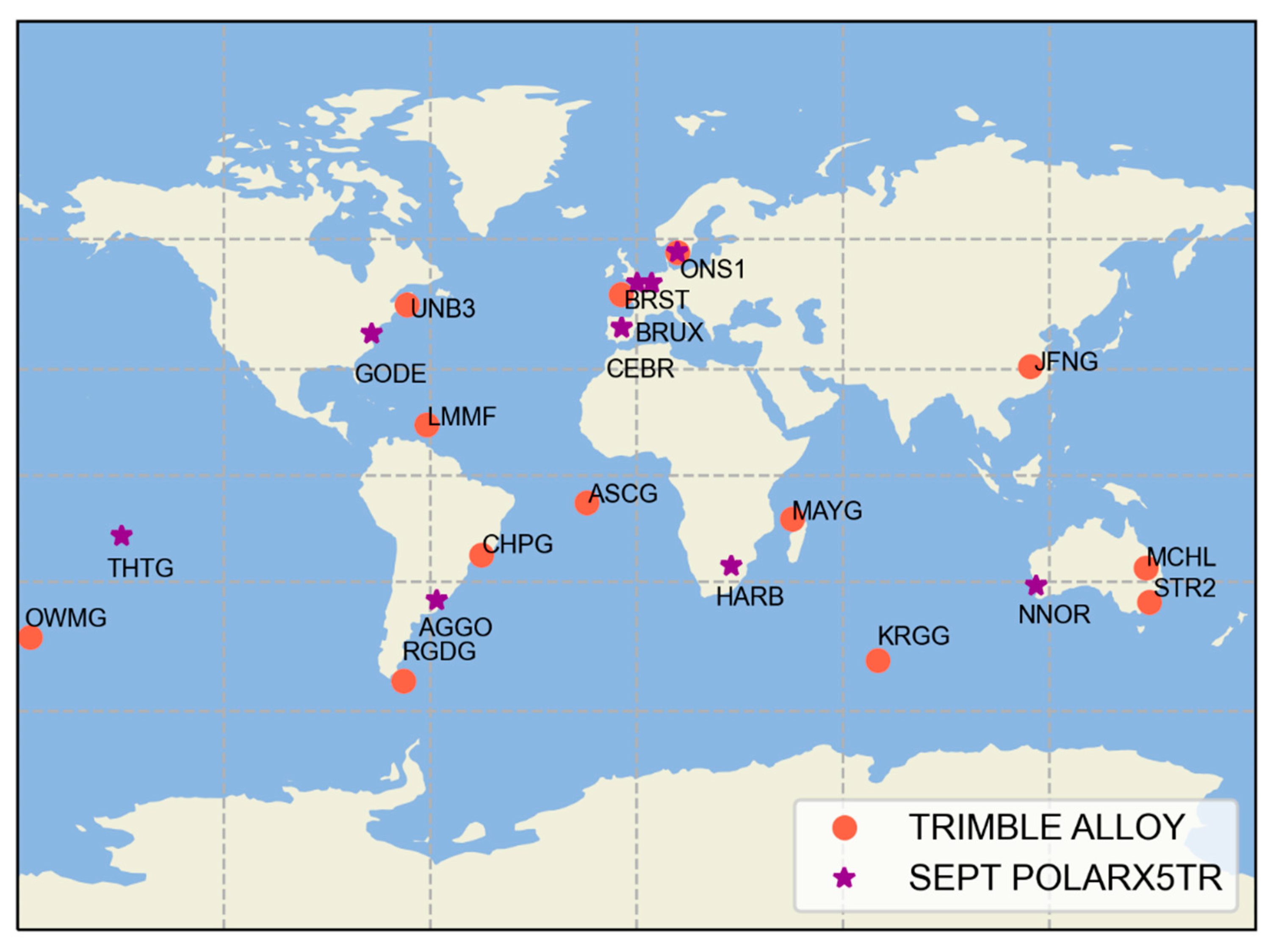
3.1. Experimental Setup

Observations for a nine-day period sampled at 30s from DOY (day of year) 001 to 009 of 2020 are processed, to access the performance of PPP AR with different AC products. As mentioned before, the Galileo PPP AR products of CNES and SGG-WHU are based on pilot signal X while pilot-data signal Q is used for CODE and PRIDE Lab products. Thus, 13 SEPT receivers were selected to access Galileo PPP AR performance which is based on signal X, while nine TRIMBLE receivers to verified the performance of signal Q. These stations are approximately uniformly distributed along the geographical latitude and longitude, as shown in Figure 1. All the PPP experiments were performed with the in-house software. In the PPP procedure, the elevation cutoff angle was set to 10 degrees. The tropospheric zenith wet delay (ZWD) was estimated as random walk noise, their spectral density values were empirically set to be 10−8 m2/s and the UAs were estimated as constants for each continuous satellite arc. The ‘GRM’,’WUM’, ‘COM’, and ‘WHU’ PPP AR products from four institutions were used to implement PPP AR. we simultaneously used the bootstrapping success rate and the ratio test to validate the integer ambiguities to lower the risk of a wrong fixing. The success rate and ratio test threshold were set as 0.95 and 2.0, respectively.
Three Groups of PPP/AR solutions were performed and compared as follows: a comparison of the float and fixed PPP solutions, GPS-only PPP AR compared among four institutions’ solutions and the contributions of multi-GNSS to PPP AR. The positioning accuracy as well as the convergence time and TTFF are analyzed and presented. In this study, the reference positions were obtained from the IGS weekly Solution Independent Exchange Format (SINEX) file and used to assess positioning performance. Here, the ‘convergence’ is defined as obtaining positioning error in east, north, up or three-dimensional (3D) direction less than the predefined threshold at the current epoch and the following twenty epochs [27,38]. The predefined dual-frequency threshold was taken as one decimeter [39].

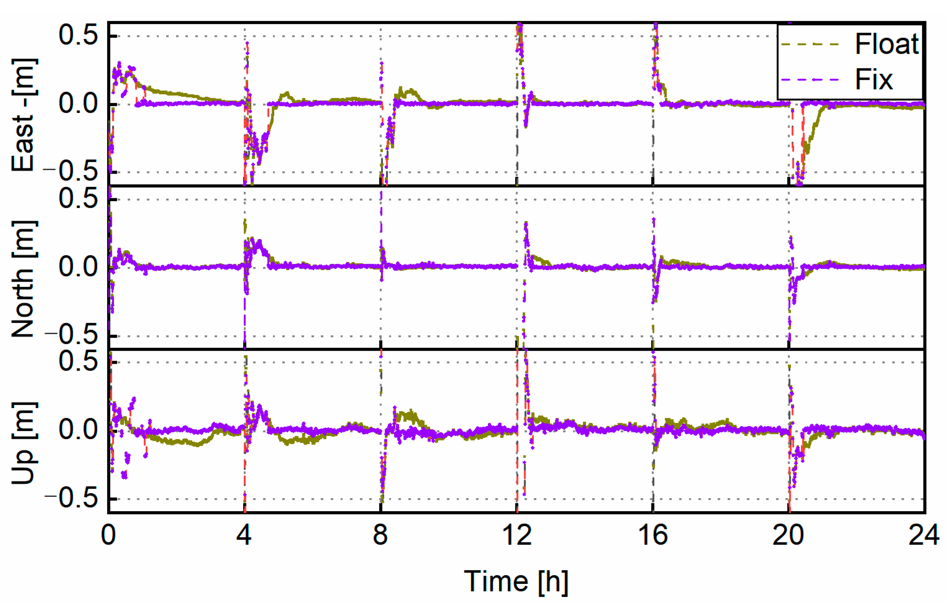
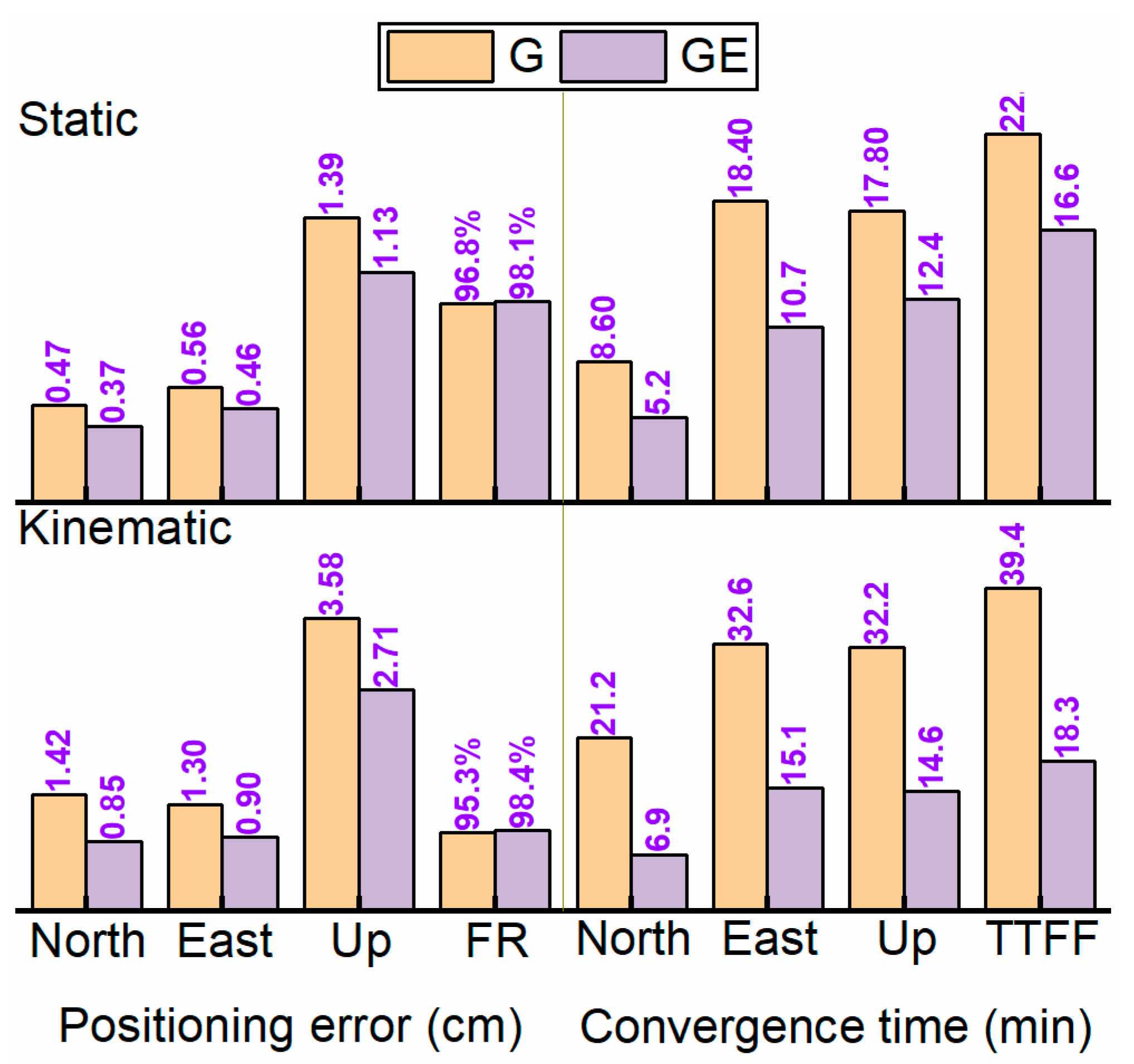
3.2. Ambiguity-Float and Fixed PPP Results

To reveal the difference between the float and fixed PPP solutions, the GPS and Galileo observations were taken as an example for comparison and analysis. The nine-day static and kinematic solutions from different stations were derived from the float and fixed PPP modes with four AC products.
First, an average of nine days GPS-only float and fixed PPP solutions of six selected stations are compared and analyzed. Figure 2 gives a representative result of kinematic PPP ambiguity-fixed solution at station AGGO. It is worth noting that the daily observation data are divided into six four-hour arcs for convenience. We can note that once the ambiguities are fixed to correct integers, the position accuracy improves significantly, especially for east and up components. Furthermore, the positioning errors in the north, east and up components derived from the static and kinematic modes with four AC products are shown in Figure 3. The test results show that the positioning accuracy varied significantly between stations. Overall, the positioning performance of both static and kinematic float PPP in the north component was better than in the other two components. After recovering the integer property of ambiguities, the positioning accuracy could be significantly improved compared to the float PPP, especially for the east component. The results with different AC products were overall consistent with each other.
To further verify the advantages of fixed PPP, we processed the data of all the stations and calculated the days and site average solutions to statistically compare the float/fixed PPP models. The positioning performance was evaluated by GPS-only as well as combined GPS and Galileo in the static and kinematic modes with four AC products. The root mean square (RMS) values of the positioning errors in the north, east and up components as well as the 3D direction are given in Figure 4 and summarized in Table 2. As shown, the GPS-only float PPP achieved 0.59, 0.94, and 1.48 cm positioning accuracy for static PPP and greater than 1.68, 2.01, and 3.97 cm for kinematic PPP in the north, east, and up components, respectively. After adding the Galileo observations, the static positioning errors could be reduced to 0.43, 0.65, and 1.28 cm, while 0.90, 1.17, and 2.72 cm for kinematic mode in the north, east, and up components, respectively.
The results also confirmed that the positioning accuracy in the east was worse than the north component and this problem could be solved by fixing the ambiguity. As shown in Figure 2, the results of both static and kinematic PPP AR could significantly be improved the positioning accuracy compared with float PPP, whether GPS-only or combined GPS and Galileo. Specifically, the static positioning errors could be reduced by 21.0% (to 0.46 cm), 52.5% (to 0.45 cm), 10.0% (to 1.33 cm) and 21.7% (to 0.33 cm), 47.4% (to 0.34 cm), 9.5% (to 1.16 cm) for GPS-only and GE combination in north, east, up component, respectively. The reductions were 20.8% (to 1.13 cm), 42.9% (to 1.15 cm), 19.9% (to 3.4 cm) and 20.4% (to 0.72 cm), 44.1% (to 0.66 cm), 10.1% (to 2.44 cm) for kinematic PPP AR. It should be noted that the statistical results were the average among the four AC PPP solutions.
In general, the positioning errors of kinematic PPP were about 2.0 to 3.0 times that of static PPP. The positioning accuracy of float-PPP could be improved by multi-GNSS combinations, meanwhile, the positioning errors can also be reduced by PPP AR effectively, especially for east components. Moreover, the float- and fixed-PPP performances with COM products provided by CODE ranked the first.

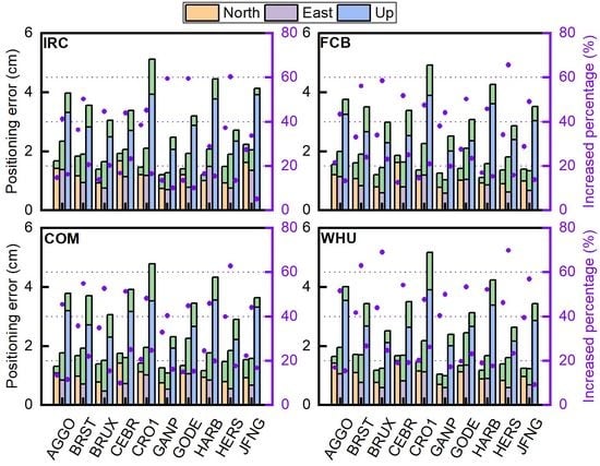
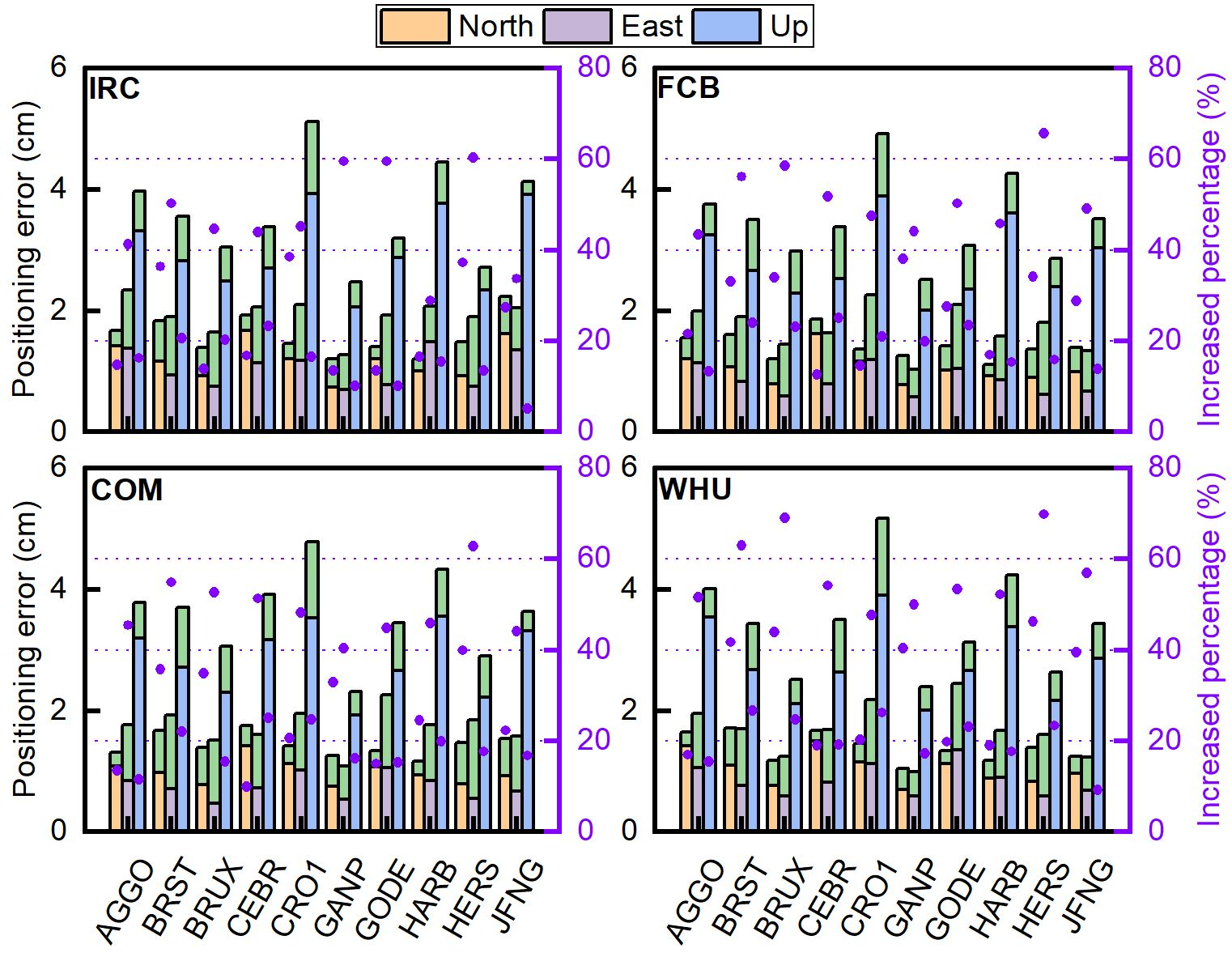
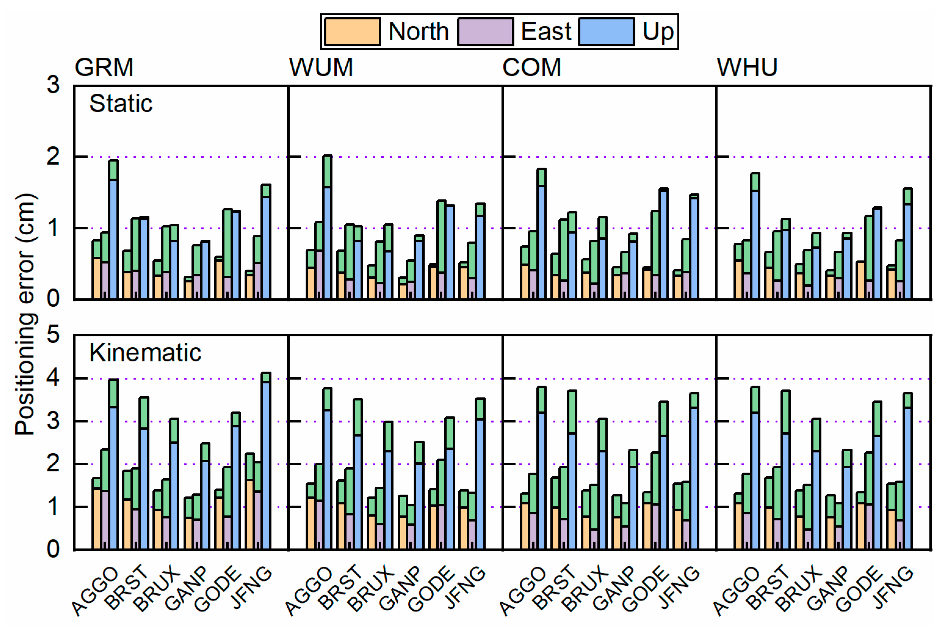
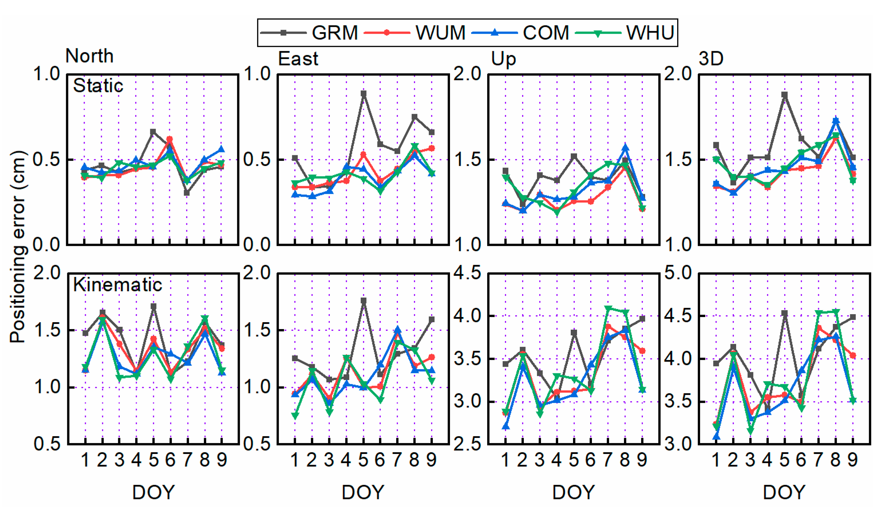
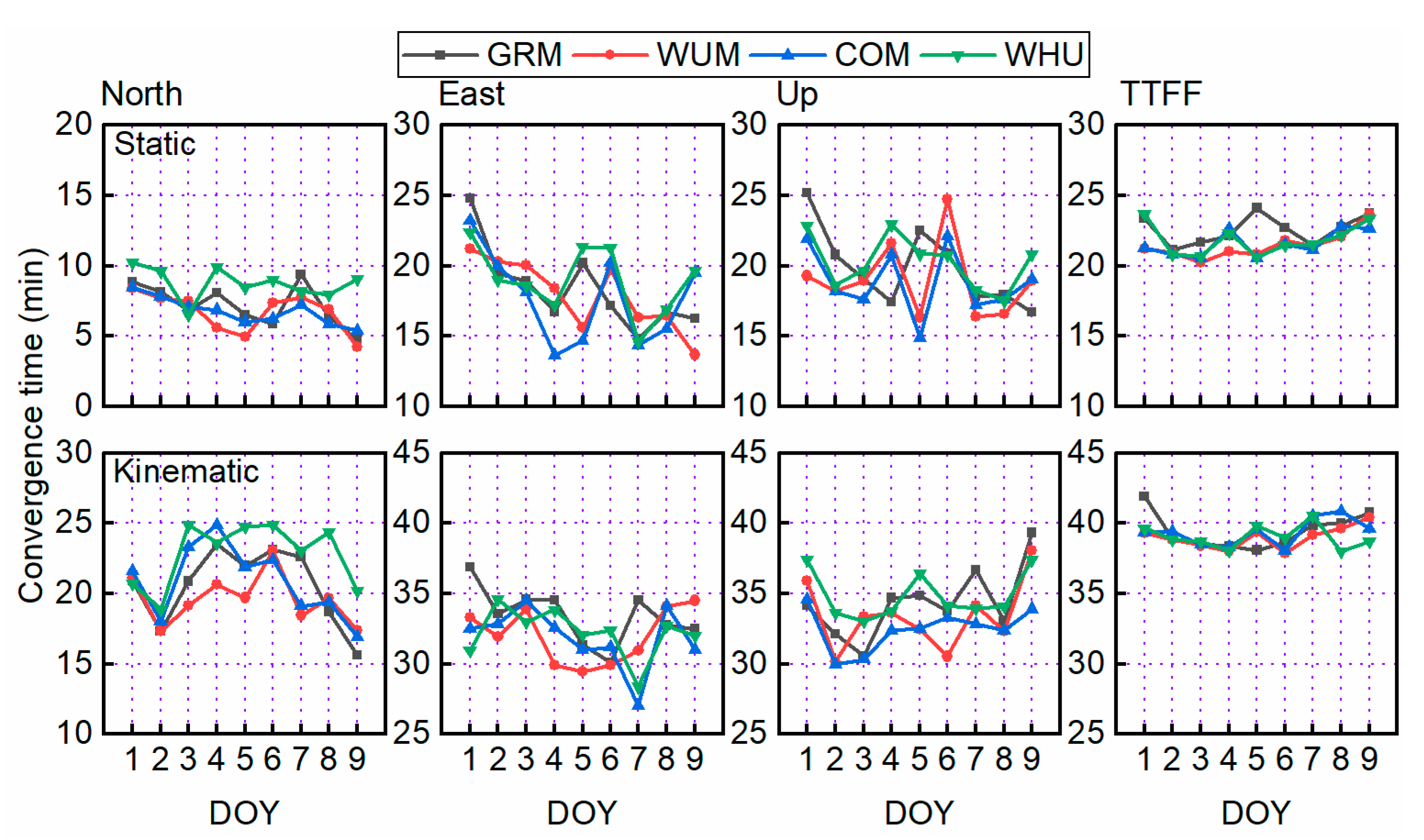
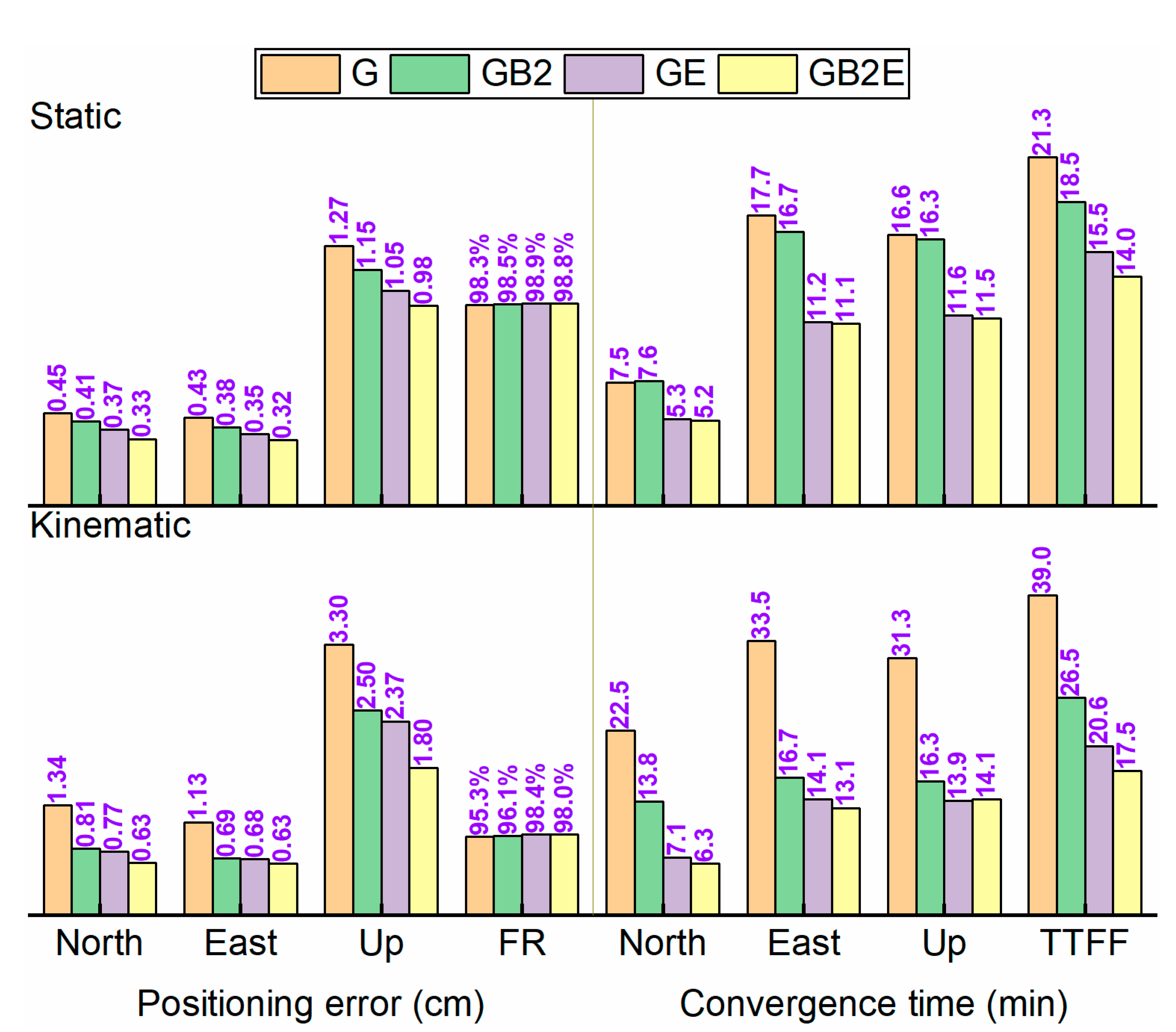
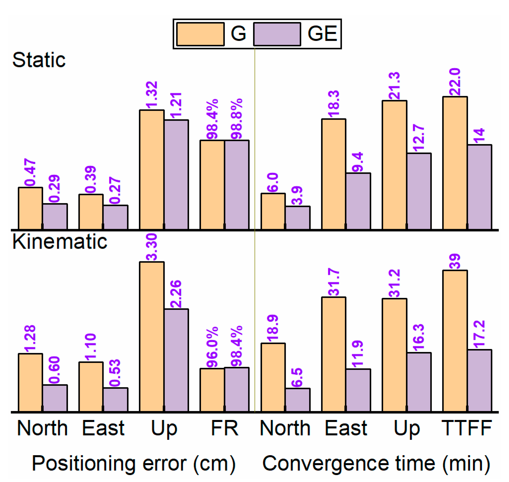
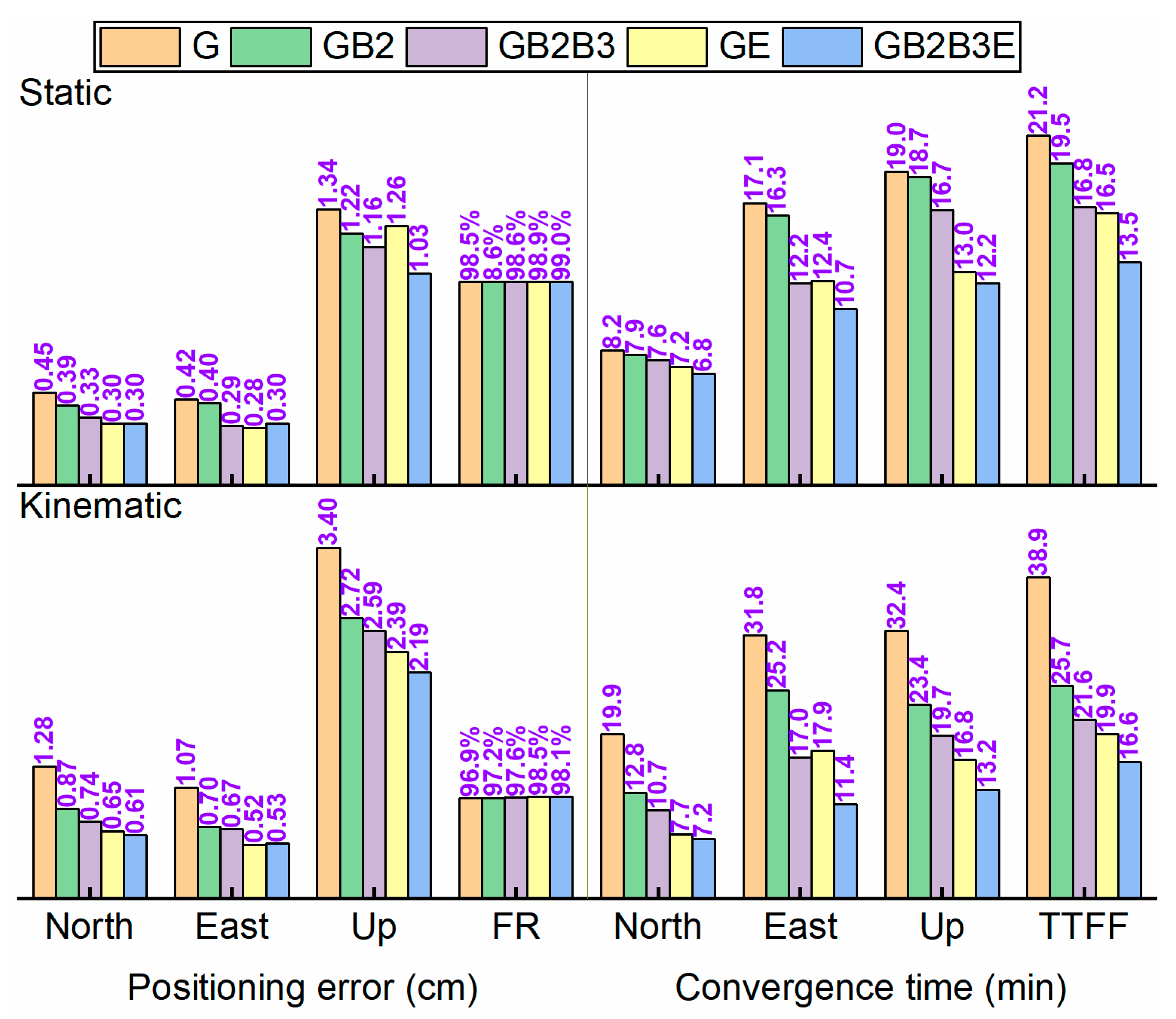
3.3. Ambiguity-Fixed Solutions from Different ACs

This section presents the results in a different form to compare the differences among fixed-PPP solutions with four AC products in detail. The solutions of all the stations from one day with different AC products were averaged and the average positioning error series among nine days are displayed in Figure 5. Besides positioning accuracy, the convergence performance and TTFF were also assessed and plotted in Figure 5. It should be noted that, to save space, only the solutions derived from GPS-only PPP AR with static and kinematic modes are presented.
Figure 5 depicts the average positioning errors derived from different AC products with static mode maintained stability among the nine days in the north, east and up components as well as in the 3D direction, respectively, except for the GRM products from CNES. This was especially the case for the east component. Previous research has indicated that WUM FCB products corresponding to CNES maintained high conformity with GRM IRC products [17]. Thus, the reasonable explanation for this phenomenon is the that PPP strategy cannot maintain good consistency with GRM products resulting in some bad station solutions, which magnifies the average positioning errors. For the kinematic situation, the average positioning errors were more volatile among the days’ solution due to the weaker model. From the Table 2, the average positioning performance among nine days with GRM, WUM, COM, and WHU products, ranging from 0.45 to 0.47 cm, from 0.39 to 0.56 cm, and from 1.27 to 1.39 cm for static GPS-only PPP AR and from 1.28 to 1.42 cm, from 1.07 to 1.3 cm, and from 3.3 to 3.6 cm for kinematic PPP AR in the north, east, and up components, respectively. Among the average positioning accuracy with the four AC products, the differences were less than 3 mm for both static and kinematic PPP AR, which shows that a comparable positioning accuracy can be achieved by using different AC products. Like the positioning performance, the convergence time shown in Figure 6 ranged from 6.70 to 8.8 min, from 17.7 to 19 min, and from 18.8 to 20.3 min for static PPP AR and from 19.6 to 22.8 min, from 31.9 to 33.4 min, and from 32.5 to 34.9 min for kinematic PPP AR in the north, east, and up components, respectively. Furthermore, TTFF was defined as the time taken for the ambiguity-fixed solution to be successfully achieved for at least five epochs, which is an important indicator to evaluate PPP AR performance. Figure 5 shows that the average TTFF of kinematic PPP AR was 39.4, 39.0, 39.4, and 38.9 min with the GRM, WUM, COM, and WHU products and it was about 2.0 times that of static PPP AR, which was 20.3, 22.6, 21.5, and 21.9 min, respectively.
In conclusion, among the positioning accuracy, convergence time and TTFF, there was no significant difference among the four AC products for PPP AR in the static or kinematic modes. This further proves the consistency among different AC products. Although the differences in positioning performance were very small, the PPP AR performance with COM products provided by CODE ranked the first, while those with the GRM product showed worse performance, which was also confirmed by Glaner and Weber [22].

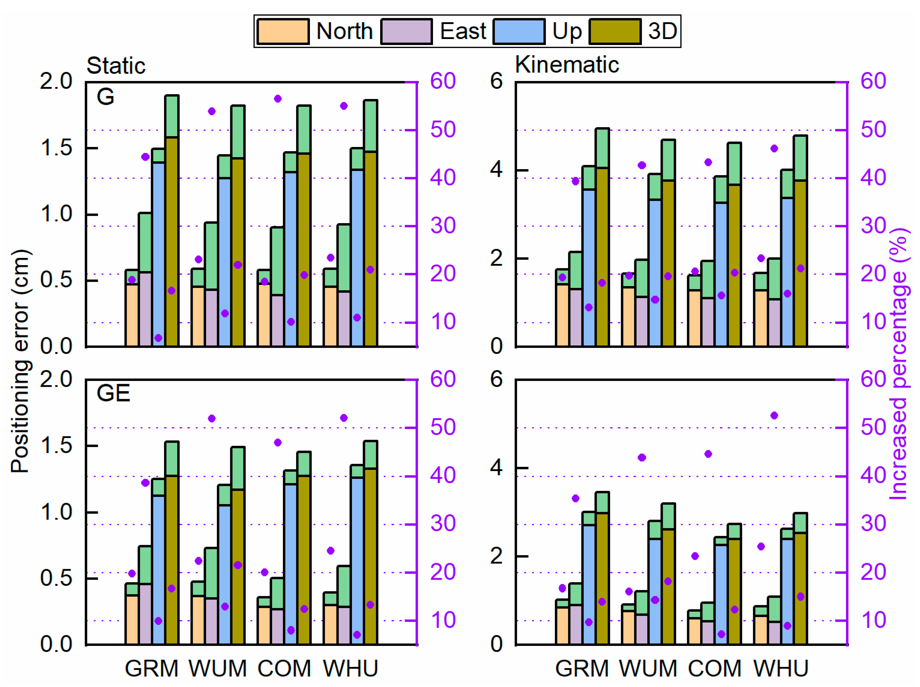
3.4. Benefit of Multi-GNSS Combination for PPP AR

Multi-GNSS observations have been demonstrated to have significant improvements in PPP performance with float solutions, not only in positioning accuracy, but also in convergence time. Studies have also shown that the TTFF and the FR of GPS PPP AR can be shortened and improved by adding observations from other GNSS. The products shown in Table 1 allow enabling PPP AR with at least two GNSS observations. To reveal the benefits of multi-GNSS for ambiguity resolution, we implemented the GPS-only and multi-GNSS combination PPP AR with different AC products. The average positioning errors, convergence time, ambiguity FR and TTFF in static and kinematic modes were evaluated with GRM, WUM, COM, and WHU products, and the statistics are shown in Figure 7, Figure 8, Figure 9 and Figure 10, respectively. The solutions from different ACs indicate that the performance of PPP AR was enhanced by more GNSS observations. Although the degree of the improvement of each AC was different after aiding by multi-GNSS, this differences in positioning accuracy, convergence time and FR as well as TTFF among the four ACs was not obvious and were within acceptable limits due to different server-side products generation strategies.
For different combinations of GNSS, the positioning accuracy of ambiguity-fixed static PPP was almost at the same level, since the unmodeled errors have less influence on the estimated precision parameters after a long time of convergence and correctly fixed ambiguities. While the positioning accuracy had more obvious improvements for kinematic PPP AR, the PPP model was strong since there were more observations. The FR was improved but not obvious among different combinations of GNSS solutions. The most significant improvements were in the convergence time and TTFF after aiding multi-GNSS. Taking kinematic mode as an example, the statistics show that typical value of convergence times were (6.9, 15.1, 14.6) min in the north, east, up components, respectively, and 18.3 min for TTFF with GRM products for the GNSS combination PPP AR. Under the same circumstances, the values were (6.3, 13.1, 14.1) min and 17.5 min for COM products, (6.5, 11.9, 16.3) min and 17.2 min for WUM products, (9.2, 17.5, 18.3) min and 20.8 min for WHU products, respectively. Figure 8 and Figure 10 show the positioning performance in terms of convergence time, positioning accuracy and TTFF derived from the static and kinematic modes, and GB2 PPP AR showed a much worse performance compared to GE PPP AR. This is because the precise orbit and clock of BDS-2 are less precise than those of GPS and Galileo. Figure 7, shows that, after adding the BDS-3 satellite to enhance GB2 PPP AR, the positioning performance was comparable with combined GPS and Galileo PPP AR. As for the combined GPS, Galileo, BD2, and BD3, the triple-GNSS PPP AR could further accelerate the convergence and shorten the TTFF.
Overall, the PPP solutions using CODE products performed best, while CNES performed notably worse. In between are the solutions using WHU and SGG products. Similar results were also reported by Zhou et al. [40] and Glaner and Weber [22].

4. Discussion

Overall, the PPP solutions using CODE products perform best, while CNES perform notably worse. In between are the solutions using WHU and SGG products. The best overall performance from CODE may be attributed to the adoption of an update solar radiation pressure (SPR) model. The satellite orbit determination and clock estimation are both affected by the modeling of SPR [40]. Therefore, the PPP with CODE products can get better float solutions, which precision will directly affect the PPP AR. On the other hand, the user-side parameters should be consistent with the server-side as much as possible, so as to maximize the effectiveness of the PPP AR products. The worse performance from CNES may be caused by inconsistent parameter settings.
Compared with short-baseline relative positioning, it is more difficult to fix all ambiguities reliably for PPP, especially for multi-GNSS PPP. A partial ambiguity resolution (PAR) method should be used to find a subset of integers which can be fixed with high confidence if fix all ambiguities is unsuccessful, which can significantly shorten TTFF and increase the fixing rate. For BDS-2 PPP AR, the elevation-dependent BDS satellite-induced code biases should be corrected following Wanninger and Beer [41]. It can be observed from the results from WUM and WHU, the GPS+BD2 PPP AR is always worse than GPS+GAL, reasonable explanation for this phenomenon is resulting in a poorer geometry of BDS-2 observations and lower products accuracy. After adding BDS-3 satellites, the performance of GPS+BDS PPP AR is enhanced.
Although there are now three forms of products to achieve PPP AR, but for PPP users, the OSB/AFC products is more convenient to use and it can be applied to ionosphere-free PPP or uncombined PPP models. ACs are strongly encouraged to perform OSB/AFC to provide users with a uniform approach to ingesting PPP AR products into their software.

5. Conclusions

The realization of PPP AR depends on the phase bias products. In this paper, three strategies for generating phase bias products were contrasted and the contribution of four institutions’ PPP AR products on GPS-only and multi-GNSS combination positioning performance retrieval with PPP AR were comprehensively investigated and evaluated based on nine days of observation of 22 MGEX stations capable of tracking GPS, Galileo, and BDS signals.
For a comparison of the float and fixed PPP solutions, once the integer property of ambiguities was recovered, the positioning accuracy could be significantly improved compared to float PPP, especially for the east component. The results with different AC products were comparable with each other. Concretely, the static positioning errors can be reduced by 21.0% (to 0.46 cm), 52.5% (to 0.45 cm), 10.0% (to 1.33 cm) and 21.7% (to 0.33 cm), 47.4% (to 0.34 cm), 9.5% (to 1.16 cm) for GPS-only and GE combination in north, east, up component, respectively, while the reductions are 20.8% (to 1.13 cm), 42.9% (to 1.15 cm), 19.9% (to 3.4 cm) and 20.4% (to 0.72 cm), 44.1% (to 0.66 cm), 10.1% (to 2.44 cm) for kinematic PPP AR.
For GPS-only fixed PPP with different AC products, among the positioning accuracy, convergence time, and TTFF, there was no significant difference among four AC products for PPP AR in the static or kinematic modes. This further proves the consistency among different AC products. Although the differences in positioning performance was very small, the PPP AR performance with COM products provided by CODE ranked the first, while those with the GRM product showed worse performance.
For multi-GNSS PPP AR, the solutions from different ACs indicate that the performance of PPP AR was enhanced by more GNSS observations. Although the degree of the improvement of each AC was different after aiding multi-GNSS, these differences in positioning accuracy, convergence time, and FR, as well as TTFF among the four ACs were not obvious and within acceptable limits due to different server-side products generation strategies. Taking kinematic mode as an example, the typical value of convergence time is (6.9, 15.1, 14.6) min in north, east, up components, respectively, and 18.3 min for TTFF with GRM products for tow GNSS combination PPP AR. Under the same circumstances, the statistics is (6.3, 13.1, 14.1) min and 17.5 min for COM products, (6.5, 11.9, 16.3) min and 17.2 min for WUM products, (9.2, 17.5, 18.3) min and 20.8 min for WHU products, respectively. While, the positioning performance in terms of convergence time, positioning accuracy and TTFF derived from the static and kinematic modes with GB2 PPP AR showed much worse performance compared to GE PPP AR.
Future work will concentrate on an uncombined PPP AR model and the inclusion of additional frequency observations. Moreover, the application of PPP AR to actual kinematic data processing will be further evaluated.

Author Contributions

Conceptualization, G.C., T.X. and G.X.; methodology, C.C.; software, C.C.; validation, C.C. and L.Y.; formal analysis, C.C.; investigation, C.C.; resources, C.C.; data curation, C.C.; writing—original draft preparation, C.C.; writing—review and editing, C.C.; visualization, C.C.; supervision, G.C., T.X. and G.X.; project administration, G.X. and G.C.; funding acquisition, G.C. All authors have read and agreed to the published version of the manuscript.

Funding

This research was funded by the National Natural Science Foundation of China grant number 42074001; 41774005; 41904039; and the Postgraduate Research & Practice Innovation Program of Jiangsu Province & China University of Mining and Technology, grant number KYCX19_2163, and the China Postdoctoral Science Foundation, grant number 2019M652010; 2019T120477.

Data Availability Statement

The source code and example data used in this study are available for free at https://github.com/heiwa0519/PPP_AR.

Acknowledgments

We would like to thank the IGS analysis centers for providing GNSS ground tracking data, precise orbit and clock products, and PPP AR products.

Conflicts of Interest

The authors declare no conflict of interest.

References

  1. Malys, S.; Jensen, P.A. Geodetic point positioning with GPS carrier beat phase data from the CASA UNO experiment. Geophys. Res. Lett. 1990, 17, 651–654. [Google Scholar] [CrossRef]
  2. Zumberge, J.; Heflin, M.; Jefferson, D.; Watkins, M.; Webb, F. Precise point positioning for the efficient and robust analysis of GPS data from large networks. J. Geophys. Res. Solid Earth 1997, 102, 5005–5017. [Google Scholar] [CrossRef] [Green Version]
  3. Zhang, H.; Gao, Z.; Ge, M.; Niu, X.; Huang, L.; Tu, R.; Li, X. On the convergence of ionospheric constrained precise point positioning (IC-PPP) based on undifferential uncombined raw GNSS observations. Sensors 2013, 13, 15708–15725. [Google Scholar] [CrossRef] [Green Version]
  4. Geng, J.; Pan, Y.; Li, X.; Guo, J.; Liu, J.; Chen, X.; Zhang, Y. Noise Characteristics of High-Rate Multi-GNSS for Subdaily Crustal Deformation Monitoring. J. Geophys. Res. Solid Earth 2018, 123, 1987–2002. [Google Scholar] [CrossRef]
  5. Su, K.; Jin, S.; Ge, Y. Rapid displacement determination with a stand-alone multi-GNSS receiver: GPS, Beidou, GLONASS, and Galileo. GPS Solut. 2019, 23, 54. [Google Scholar] [CrossRef]
  6. Lu, C.; Li, X.; Nilsson, T.; Ning, T.; Heinkelmann, R.; Ge, M.; Glaser, S.; Schuh, H. Real-time retrieval of precipitable water vapor from GPS and BeiDou observations. J. Geod. 2015, 89, 843–856. [Google Scholar] [CrossRef]
  7. Gao, Y.; Shen, X. A New Method for Carrier-Phase-Based Precise Point Positioning. Navigation 2002, 49, 109–116. [Google Scholar] [CrossRef]
  8. Gao, Z.; Zhang, H.; Ge, M.; Niu, X.; Shen, W.; Wickert, J.; Schuh, H. Tightly coupled integration of multi-GNSS PPP and MEMS inertial measurement unit data. GPS Solut. 2017, 21, 377–391. [Google Scholar] [CrossRef]
  9. Li, X.; Ge, M.; Guo, B.; Wickert, J.; Schuh, H. Temporal point positioning approach for real-time GNSS seismology using a single receiver. Geophys. Res. Lett. 2013, 40, 5677–5682. [Google Scholar] [CrossRef] [Green Version]
  10. Calais, E.; Han, J.; DeMets, C.; Nocquet, J. Deformation of the North American plate interior from a decade of continuous GPS measurements. J. Geophys. Res. Solid Earth 2006, 111. [Google Scholar] [CrossRef] [Green Version]
  11. Geng, J.; Chen, X.; Pan, Y.; Mao, S.; Li, C.; Zhou, J.; Zhang, K. PRIDE PPP-AR: An open-source software for GPS PPP ambiguity resolution. GPS Solut. 2019, 23. [Google Scholar] [CrossRef]
  12. Xiao, G.; Li, P.; Gao, Y.; Heck, B. A unified model for multi-frequency PPP ambiguity resolution and test results with Galileo and BeiDou triple-frequency observations. Remote Sens. 2019, 11, 116. [Google Scholar] [CrossRef] [Green Version]
  13. Ge, M.; Gendt, G.; Rothacher, M.; Shi, C.; Liu, J. Resolution of GPS carrier-phase ambiguities in Precise Point Positioning (PPP) with daily observations. J. Geod. 2008, 82, 389–399. [Google Scholar] [CrossRef]
  14. Collins, P.; Bisnath, S.; Lahaye, F.; Héroux, P. Undifferenced GPS ambiguity resolution using the decoupled clock model and ambiguity datum fixing. Navigation 2010, 57, 123–135. [Google Scholar] [CrossRef] [Green Version]
  15. Laurichesse, D.; Mercier, F.; BERTHIAS, J.P.; Broca, P.; Cerri, L. Integer ambiguity resolution on undifferenced GPS phase measurements and its application to PPP and satellite precise orbit determination. J. Navig. 2009, 56, 135–149. [Google Scholar] [CrossRef]
  16. Duan, B.; Hugentobler, U.; Selmke, I.; Wang, N. Estimating ambiguity fixed satellite orbit, integer clock and daily bias products for GPS L1/L2, L1/L5 and Galileo E1/E5a, E1/E5b signals. J. Geod. 2021, 95, 44. [Google Scholar] [CrossRef]
  17. Hu, J.; Zhang, X.; Li, P.; Ma, F.; Pan, L. Multi-GNSS fractional cycle bias products generation for GNSS ambiguity-fixed PPP at Wuhan University. GPS Solut. 2019, 24, 15. [Google Scholar] [CrossRef]
  18. Li, P.; Jiang, X.; Zhang, X.; Ge, M.; Schuh, H. GPS + Galileo + BeiDou precise point positioning with triple-frequency ambiguity resolution. GPS Solut. 2020, 24, 78. [Google Scholar] [CrossRef]
  19. Li, X.; Han, X.; Li, X.; Liu, G.; Feng, G.; Wang, B.; Zheng, H. GREAT-UPD: An open-source software for uncalibrated phase delay estimation based on multi-GNSS and multi-frequency observations. GPS Solut. 2021, 25, 66. [Google Scholar] [CrossRef]
  20. Xiao, G.; Sui, L.; Heck, B.; Zeng, T.; Tian, Y. Estimating satellite phase fractional cycle biases based on Kalman filter. GPS Solut. 2018, 22, 82. [Google Scholar] [CrossRef]
  21. Liu, G.; Guo, F.; Wang, J.; Du, M.; Qu, L. Triple-Frequency GPS Un-Differenced and Uncombined PPP Ambiguity Resolution Using Observable-Specific Satellite Signal Biases. Remote Sens. 2020, 12, 2310. [Google Scholar] [CrossRef]
  22. Glaner, M.; Weber, R. PPP with integer ambiguity resolution for GPS and Galileo using satellite products from different analysis centers. GPS Solut. 2021, 25, 102. [Google Scholar] [CrossRef]
  23. Geng, J.; Chen, X.; Pan, Y.; Zhao, Q. A modified phase clock/bias model to improve PPP ambiguity resolution at Wuhan University. J. Geod. 2019, 93, 2053–2067. [Google Scholar] [CrossRef]
  24. Geng, J.; Meng, X.; Dodson, A.H.; Teferle, F.N. Integer ambiguity resolution in precise point positioning: Method comparison. J. Geod. 2010, 84, 569–581. [Google Scholar] [CrossRef] [Green Version]
  25. Shi, J.; Gao, Y. A comparison of three PPP integer ambiguity resolution methods. GPS Solut. 2013, 18, 519–528. [Google Scholar] [CrossRef]
  26. Banville, S.; Geng, J.; Loyer, S.; Schaer, S.; Springer, T.; Strasser, S. On the interoperability of IGS products for precise point positioning with ambiguity resolution. J. Geod. 2020, 94, 10. [Google Scholar] [CrossRef]
  27. Zhou, F.; Dong, D.; Li, W.; Jiang, X.; Wickert, J.; Schuh, H. GAMP: An open-source software of multi-GNSS precise point positioning using undifferenced and uncombined observations. GPS Solut. 2018, 22, 33. [Google Scholar] [CrossRef]
  28. Kouba, J. A Guide to Using International GNSS Service (IGS) Products. Available online: https://kb.igs.org/hc/en-us/articles/201271873-A-Guide-to-Using-the-IGS-Products (accessed on 12 August 2021).
  29. Peng, Y.; Scales, W.A.; Hartinger, M.D.; Xu, Z.; Coyle, S. Characterization of multi-scale ionospheric irregularities using ground-based and space-based GNSS observations. Satell. Navig. 2021, 2, 14. [Google Scholar] [CrossRef]
  30. Zhao, L.; Ye, S.; Song, J. Handling the satellite inter-frequency biases in triple-frequency observations. Adv. Space Res. 2017, 59, 2048–2057. [Google Scholar] [CrossRef]
  31. Liu, S.; Sun, F.; Zhang, L.; Li, W.; Zhu, X. Tight integration of ambiguity-fixed PPP and INS: Model description and initial results. GPS Solut. 2016, 20, 39–49. [Google Scholar] [CrossRef]
  32. Dong, D.N.; Bock, Y. Global Positioning System network analysis with phase ambiguity resolution applied to crustal deformation studies in California. J. Geophys. Res. Solid Earth 1989, 94, 3949–3966. [Google Scholar] [CrossRef]
  33. Teunissen, P.; De Jonge, P.; Tiberius, C. The LAMBDA method for fast GPS surveying. In Proceedings of the International Symposium “GPS Technology Applications”, Bucharest, Romania, 26–29 September 1995. [Google Scholar]
  34. Chang, X.-W.; Yang, X.; Zhou, T. MLAMBDA: A modified LAMBDA method for integer least-squares estimation. J. Geod. 2005, 79, 552–565. [Google Scholar] [CrossRef] [Green Version]
  35. Bakuła, M. Instantaneous Ambiguity Reinitialization and Fast Ambiguity Initialization for L1-L2 GPS Measurements. Sensors 2020, 20, 5730. [Google Scholar] [CrossRef] [PubMed]
  36. Li, P.; Zhang, X.; Ren, X.; Zuo, X.; Pan, Y. Generating GPS satellite fractional cycle bias for ambiguity-fixed precise point positioning. GPS Solut. 2015, 20, 771–782. [Google Scholar] [CrossRef]
  37. Villiger, A.; Schaer, S.; Dach, R.; Prange, L.; Sušnik, A.; Jäggi, A. Determination of GNSS pseudo-absolute code biases and their long-term combination. J. Geod. 2019, 93, 1487–1500. [Google Scholar] [CrossRef]
  38. Li, X.; Zhang, X.; Guo, F. Predicting atmospheric delays for rapid ambiguity resolution in precise point positioning. Adv. Space Res. 2014, 54, 840–850. [Google Scholar] [CrossRef]
  39. Lou, Y.; Zheng, F.; Gu, S.; Wang, C.; Guo, H.; Feng, Y. Multi-GNSS precise point positioning with raw single-frequency and dual-frequency measurement models. GPS Solut. 2015, 20, 849–862. [Google Scholar] [CrossRef]
  40. Zhou, F.; Cao, X.; Ge, Y.; Li, W. Assessment of the positioning performance and tropospheric delay retrieval with precise point positioning using products from different analysis centers. GPS Solut. 2019, 24, 12. [Google Scholar] [CrossRef]
  41. Wanninger, L.; Beer, S. BeiDou satellite-induced code pseudorange variations: Diagnosis and therapy. GPS Solut. 2015, 19, 639–648. [Google Scholar] [CrossRef] [Green Version]
Figure 1. Ground tracking stations, red dots denote 13 SEPT receivers tracking GPS/Galileo Q signals, stars represent 9 TRIMBLE receivers tracking GPS/Galileo X signals.
Remotesensing 13 03266 g001
Figure 2. The positioning error at station AGGO with kinematic mode in north, east, up components.
Remotesensing 13 03266 g002
Figure 3. The positioning error of GPS-only float/fixed PPP solutions with static (top) and kinematic (bottom) mode in north, east, up components of nine days average for different stations with GRM, WUM, COM, and WHU products. The orange, purple, and blue bar denote fixed PPP solution in north, east, and up components, which plus green bar represents the corresponding float PPP solution.
Remotesensing 13 03266 g003
Figure 4. Averaged positioning error of GPS-only and GE float/fixed PPP static (left) and kinematic (right) in north, east, up, and 3D components with GRM, WUM, COM, and WHU products. The orange, purple, blue, and brown pillar denotes fixed PPP solution in north, east, up, and 3D components, which plus green pillar represents the corresponding float PPP solution. The blue dots show the increased percentage of the fixed solution compared to the float.
Remotesensing 13 03266 g004
Figure 5. Average positioning errors series among nine days of static (top) and kinematic (bottom) GPS-only PPP AR in north, east, up, and 3D components with GRM, WUM, COM, and WHU products.
Remotesensing 13 03266 g005
Figure 6. Average convergence time series among nine days of static (top) and kinematic (bottom) GPS-only PPP AR in north, east, up, and 3D components with GRM, WUM, COM, and WHU products.
Remotesensing 13 03266 g006
Figure 7. Average performance of multi-GNSS PPP AR in static (top) and kinematic (bottom) mode with GRM products. FR is defined as the ratio of the number of fixed epochs to the number of total epochs after TTFF and TTFF means time to first fix. The specific value is recorded at the top of the bar.
Remotesensing 13 03266 g007
Figure 8. Average performance of multi-GNSS PPP AR in static (top) and kinematic (bottom) mode with WUM products. FR is defined as the ratio of the number of fixed epochs to the number of total epochs after TTFF and TTFF means time to first fix. The specific value is recorded at the top of the bar.
Remotesensing 13 03266 g008
Figure 9. Average performance of multi-GNSS PPP AR in static (top) and kinematic (bottom) mode with COM products. FR is defined as the ratio of the number of fixed epochs to the number of total epochs after TTFF and TTFF means time to first fix. The specific value is recorded at the top of the bar.
Remotesensing 13 03266 g009
Figure 10. Average performance of multi-GNSS PPP AR in static (top) and kinematic (bottom) mode with WHU products. FR is defined as the ratio of the number of fixed epochs to the number of total epochs after TTFF and TTFF means time to first fix. The specific value is recorded at the top of the bar.
Remotesensing 13 03266 g010
Table 1. An overview of the PPP AR products of the end of May 2021 (The websites were accessed on 16 August 2021).
InstitutionFormConstellationAvailable
CNES (GRM)WSB+IRCGR*Eftp://igs.ign.fr/pub/igs/products
WUMWL/NL FCBGR*EB2Jhttps://github.com/FCB-SGG
CODE (COM)OSB/AFCGR*EB2*http://ftp.aiub.unibe.ch/CODE/
PRIDE (WHU)OSB/AFCGR*EB2B3ftp://igs.gnsswhu.cn/
The letters G, R, E, B2, B3, and J, denote, respectively, GPS, GLONASS, Galileo, BeiDou-2, BeiDou-3, and QZSS. The same letters will be used below. The systems with a star symbol indicate that PPP AR products of this system are not provided.
Table 2. The means RMS (cm) of GPS-only and GE float/fixed PPP static/kinematic positioning errors with four ACs products, where N means the north component, the E means east component, and U means the up component.
StaticKinematic
FloatFixFloatFix
NEUNEUNEUNEU
GRM0.581.001.500.470.561.391.762.154.091.421.33.6
WUM0.590.941.440.450.431.271.671.973.901.341.133.3
COM0.580.901.470.470.391.321.611.943.861.281.13.3
WHU0.590.931.510.450.421.341.672.004.011.281.073.4
GRM0.460.751.250.370.461.131.021.393.000.850.902.71
WUM0.480.731.210.370.351.050.921.212.800.770.682.40
COM0.360.511.320.290.271.210.780.962.440.600.532.26
WHU0.400.591.350.30.281.260.871.102.630.650.522.39
Publisher’s Note: MDPI stays neutral with regard to jurisdictional claims in published maps and institutional affiliations.

