Article

Tracking of Multiple Maneuvering Random Hypersurface Extended Objects Using High Resolution Sensors

1
School of Information Engineering, Henan University of Science and Technology, Luoyang 471023, China
2
School of Information and Communication Engineering, University of Electronic Science and Technology of China, Chengdu 611731, China
3
Faculty of Electronic and Information Engineering, Xi’an Jiaotong University, Xi’an 710049, China
*
Author to whom correspondence should be addressed.
Remote Sens. 2021, 13(15), 2963; https://doi.org/10.3390/rs13152963
Submission received: 2 June 2021 / Revised: 15 July 2021 / Accepted: 20 July 2021 / Published: 28 July 2021

Abstract

:
With the increased resolution capability of modern sensors, an object should be considered as extended if the target extent is larger than the sensor resolution. Multiple maneuvering extended object tracking (MMEOT) uses not only measurements of the target centroid but also high-resolution sensor measurements which may resolve individual features or measurement sources. MMEOT aims to jointly estimate object number, centroid states, and extension states. However, unknown and time-varying maneuvers of multiple objects produce difficulties in terms of accurate estimation. For multiple maneuvering star-convex extended objects using random hypersurface models (RHMs) in particular, their complex maneuvering behaviors are difficult to be described accurately and handled effectively. To deal with these problems, this paper proposes an interacting multiple model Gaussian mixture probability hypothesis density (IMM-GMPHD) filter for multiple maneuvering extended object tracking. In this filter, linear maneuver models derived from RHMs are utilized to describe different turn maneuvers of star-convex extended objects accurately. Based on these, an IMM-GMPHD filtering recursive form is given by deriving new update and merging formulas of model probabilities for extended objects. Gaussian mixture components of different posterior intensities are also pruned and merged accurately. More importantly, the geometrical significance of object extension states is fully considered and exploited in this filter. This contributes to the accurate estimation of object extensions. Simulation results demonstrate the effectiveness of the proposed tracking approach—it can obtain the joint estimation of object number, kinematic states, and object extensions in complex maneuvering scenarios.

1. Introduction

In recent years, extended object tracking has attracted more attention and has been applied widely in many practical situations [1,2,3,4] (e.g., airplane tracking, vehicle tracking, and so on). Conventional multiple target tracking approaches [5,6] usually model targets as point targets. A single point target is assumed to generate at most one measurement. The combinatorial nature between targets and measurements is followed to track multiple targets. However, data associations between measurements and targets usually cause intractable computation loads for these approaches. To deal with this problem, a probability hypothesis density (PHD) filter [7,8] and its variations [9,10,11,12] were proposed based on the finite set statistics (FISST) theory. In these filters, targets’ states and measurements are modeled using random finite sets (RFS), which eliminates the complex calculation of data associations.
With the development of high-resolution sensors, a target may have multiple scattering centers (also called measurement sources). Correspondingly, multiple measurements may be taken from these scattering centers. Such a target is defined as an extended object [13,14], and vivid information (e.g., object shape and size) of an extended object can be obtained from its measurements. For multiple extended object tracking (MEOT) approaches, there are two main categories. The first category simplifies the tracking problem of MEOT by ignoring the geometrical shapes of extended objects. In these approaches, the set of measurements from extended objects is a cluster without any geometric significance. Specifically, the measurement number of an extended object is assumed to obey a Poisson distribution [15] and the distribution of these measurements is determined by a so-called inhomogeneous Poisson point process measurement model [16]. Considering these assumptions, many MEOT approaches were proposed in the PHD framework, such as an extended target probability hypothesis density (ET-PHD) filter [17] and an extended target Gaussian mixture probability hypothesis density (ET-GM-PHD) filter [18]. It is noted that these filters only focus on estimating object number and kinematic states without considering the object extension estimation.
Another category of MEOT approaches models object extensions to estimate extension-involved states (e.g., objects’ shapes, orientations, and sizes). One of the extended object modeling approaches is the random matrix approach [19,20,21,22], in which elliptic shape is described as a random symmetric positive definite matrix. By adopting this approach, a Gaussian-inverse Wishart probability hypothesis density (GIW-PHD) filter and a gamma Gaussian-inverse Wishart probability hypothesis density (GGIW-PHD) filter were proposed for tracking multiple elliptic extended objects. Nevertheless, these filters could not handle the tracking of extended objects with extensions more complex than ellipses. To solve this problem, a so-called random hypersurface model (RHM) [23,24] was proposed, which can track not only simple elliptic objects but also extended objects with complex extensions (e.g., star-convex shapes). Based on RHMs, a variation [25] of the ET-GM-PHD filter was proposed for tracking multiple star-convex extended objects. However, its merging step may not fully consider the geometric significance of extension-involved states, which may lead to the degradation of extension estimate performance. Additionally, the maneuvering behaviors of multiple star-convex extended objects may not be solved effectively in this filter.
Considering RHM’s flexibility to describe complex extensions, this paper focuses on multiple maneuvering star-convex extended object tracking (MMSEOT) using RHMs. For MMSEOT using RHMs, complex maneuvering behaviors of star-convex extended objects are difficult to be described and managed accurately. The maneuvering behaviors of a star-convex extended object using RHM are hard to be modeled by a simple mathematical form due to the tight couple between the dynamic evolution of centroid-involved kinematical parameters and that of extension-involved parameters. What is worse, maneuver models of multiple star-convex extended objects are typically unknown and time-varying, which brings significant challenges for MMSEOT. Though the interacting multiple model (IMM) approach and its variations [26,27,28,29,30,31] seem promising for handling the unknown maneuver models of objects, the model probability update step of these approaches is unfit for MMSEOT. Moreover, these approaches do not consider the estimation of object extensions.
To deal with above problems of MMSEOT using RHMs, an IMM-GMPHD filter is proposed to jointly estimate the object number, centroid dynamics, and extensions of maneuvering star-convex extended objects. To describe different turn maneuvers (with distinct turn rates and directions) of star-convex extended objects, linear maneuver models are integrated to RHMs. These maneuver models can effectively handle the tight couple between the evolution of centroid-involved kinematical states and that of extension-involved states. Thanks to their simple forms, they are easily applied to the IMM-GMPHD filter. To handle the uncertainty of maneuver models, a complete filtering recursion of the proposed filter is formed by adjusting the filtering procedures of both the ET-GM-PHD filter and IMM approach. It strictly derives update formulas of model probabilities for extended objects. More importantly, a new merging and pruning strategy of model probabilities is proposed, which greatly contributes to obtaining the accurate posterior intensity function of extended objects. Furthermore, this filter also proposes a merging and pruning strategy of Gaussian mixture components. The merging of means in Gaussian mixture components is divided into two parts, i.e., the merging of centroid kinematical parameters and the merging of extension-involved parameters. For extension-involved parameters in particular, they cannot be directly merged owing to their geometric meanings. Thus, the merging of extension-involved parameters is turned to that of values of radial functions, which supports achieving more accurate extension estimations to a great extent. Simulation results illustrated that the proposed filter obtains better estimation performance in centroid dynamics and object extensions compared with the traditional multiple extended object tracking approach based on RHMs, especially when objects maneuver simultaneously. The innovations of this work can be further summarized as follows.
(1) The maneuver models of star-convex extended objects can accurately describe turn maneuvers with different turn rates and be easily implemented in the IMM-GMPHD filter due to their concise and linear mathematical forms;
(2) The update and merging formulas of model probabilities are strictly derived in the proposed filter, which facilitates the accurate tracking of multiple extended objects with unknown and time-varying maneuvering behaviors;
(3) The geometrical significance of extension-involved states is fully considered in the merging process of Gaussian mixture components to improve the extension estimation performance;
(4) By propagating the intensity function of multiple extended objects, the proposed IMM-GMPHD filtering recursion achieves the joint estimation of object number, centroid states, and object extensions accurately in complex maneuvering tracking scenarios.
The structure of this paper is as follows: Section 2 primarily analyzes problems in multiple maneuvering extended objects tracking. Section 3 proposes an IMM-GMPHD filter for MMSEOT. This section minutely mentions maneuver models for star-convex extended objects, update formulas of model probabilities for maneuvering extended objects, and specific filtering steps of the proposed filter. In Section 4, simulation results are presented to highlight the effectiveness of the proposed filter. The last section concludes this paper.

2. Problem Formulation

In MMSEOT, the state vector ξ k of a maneuvering extended object contains not only dynamic parameters x k , m (e.g., positions [ x k , y k ] T and velocities [ x ˙ k , y ˙ k ] T in a two-dimensional Cartesian coordinate system) about the centroid but also parameters x k , e involving the object extension (e.g., the shape and orientation). It is crucial to note that objects with different extensions (e.g., ellipses, circles, and star shapes) solely have different x k , e , i.e., x k , e totally depends on the specific spatial extension of an extended object. Here, we focus on maneuvering star-convex extended objects using RHMs.

2.1. System Models of A Star-Convex Extended Object

Dynamic Model: As mentioned above, the whole state for a star-convex extended object is denoted by
ξ k = x k , e x k , m T
The dynamic equation of an object state justifies the evolution of centroid-involved kinematical variables x k , m and that of extension-involved variables x k , e simultaneously, which has the following form:
ξ k + 1 = F k , e 0 0 F k , m x k , e x k , m + w k , e w k , m
where F k , e and F k , m denote transition matrices for x k , e and x k , m , respectively, and w k , e and w k , m represent process noises for x k , e and x k , m , respectively.
It is significant that when a star-shape extended object maneuvers with a constant turn motion, mathematical representations of F k , e and F k , m are complex and difficult to calculate. This is because the rotation of the object extension simultaneously occurs with that of the centroid, resulting in the tight couple between the evolution of x k , e and x k , m . Moreover, it may be hard to describe different maneuvering behaviors of the object by a uniform form of F k , e and F k , m .
Measurement Model: The measurement model is used to describe the sensor measurement generation process of an object. An extended object with a specific extension may have multiple scattering points (also identified as measurement sources) at per scan of a high-resolution sensor. In this situation, the measurement model of an extended object is usually composed of two parts:
(1) Extension Model: This specifies the locations of measurement sources.
(2) Sensor Model: This produces measurements from measurement sources via a sensor noise, i.e.,
z k i = y k i + v k i .
where y k i is the i t h measurement source, z k i is the measurement obtained by y k i , and v k i is the sensor noise.
For a star-convex extended object, the entire measurement generation process is illustrated in Figure 1. Here the extension of a star-convex object is modeled by the RHM. The object shape boundary is denoted by S ξ k . The measurement source lies on a random scaled contour S ¯ ξ k of this extended object. The scaled version of S ξ k for a star-convex object can be calculated by a scaling factor s k (modeled as a one-dimensional random variable). If s k = 1 , the scaled boundary is exactly equal to the object shape boundary S ξ k . Thus, using scaled contours aids in successfully covering the measurement sources lying in the interior of the boundary as well as on the boundary.
With the help of a radial function r θ (which gives the distance between the centroid x k , c and a contour point), the polar representation of the scaled contour S ¯ ξ k is derived by
S ¯ ξ k = s k r θ e θ + x k , c θ 0 , 2 π , s k 0 , 1
where e θ = cos θ sin θ , θ represents the angle between the vector from the centroid to a contour point and the x-axis.
Using Fourier series expansion of degree N F , the radial function r θ has the following finite dimensional parameterizable form:
r B k , θ = a k 0 2 + j = 1 N F a k j cos j θ + b k j sin j θ = R θ B k
where
R θ = 1 , cos θ , sin θ , , cos N F θ , sin N F θ
B k = a k 0 , a k 1 , b k 1 , , a k N F , b k N F
Here, B k is considered to be extended-involved parameters x k , e in the state ξ k , i.e.,
x k , e = a k 0 , a k 1 , b k 1 , , a k N F , b k N F .
Substituting Equation (5) into Equation (4) yields the following representation of S ¯ ξ k :
S ¯ ξ k = s k R θ B k e θ + x k , c θ 0 , 2 π , s k 0 , 1
Then, the measurement source y k ( i ) can be drawn from S ¯ ξ k , i.e.,
y k ( i ) s k , i R θ k , i B k e θ k , i + x k , c
where s k , i is a random draw from s k , and θ k , i is the angle between the vector from the centroid to y k ( i ) and the x-axis.
Following the sensor model as explained in Equation (3), the measurement equation can be derived by
z k i = y k i + v k i = s k , i R θ k , i B k e θ k , i + x k , c + v k i
Nevertheless, the angle θ k , i is practically unknown. The angle ϕ k , i between the vector from the current centroid estimation to the observed measurement and the x-axis is used to approximate θ k , i . To minimize the effect of approximating ϕ k , i with θ k , i , the measurement equation can be converted into the following form, which maps the state ξ k , measurement noise v k i , scaling factor s k , i , and observed measurement z k i to a pseudo-measurement 0:
0 = h * ( ξ k , v k i , s k , i , z k i ) = s k , i 2 R ϕ k , i R ϕ k , i 2 + 2 s k , i R ϕ k , i B k e ϕ k , i v k i + v k i 2 z k i x k , c 2

2.2. Multiple Extended Object Tracking Framework

In traditional multiple extended object tracking scenarios, object number is mostly unknown, and not all objects are detected by sensors. This implies that some objects in the surveillance area may remain undetected, and their corresponding measurements are not observed. Apart from the observed measurements from objects, there are clutters in the tracking scenarios, which introduces difficulty in jointly tracking multiple objects. Here, the measurements from objects are indistinguishable from clutters, and the order of measurements is listed without any specific significance. This implies that the association between objects, clutters, and measurements is uncertain.
To jointly track multiple extended objects, measurements and states at each time step are modeled as RFSs, respectively. This avoids complex data associations between objects and measurements. Derived from the GM-PHD filter, an ET-GM-PHD filter [18] was proposed for multiple extended object tracking. In the ET-GM-PHD filter, the measurement generation process is modeled using spatial distribution models [16]. It indicates that the state x k to be estimated only contains kinematical variables (e.g., positions and velocities). Similar to the GM-PHD filter, the ET-GM-PHD filter also propagates the posterior intensity of RFS of extended objects by prediction and update steps. The prediction step here is the same as that of the GM-PHD filter. Unlike the update step in the GM-PHD filter, the partitioning results of measurements are used to update the predicted Gaussian mixture components in the ET-GM-PHD filter. Here, the update step in the ET-GM-PHD filter is to be noticed, which is summarized as follows.
It is assumed that the RFSs of object states and measurements at time step k are denoted by X k = x k i i = 1 N x , k and Z k = z k j j = 1 N z , k , respectively. Here, N x , k is the number of objects, and N z , k is the number of observed measurements. Different partitions (each of which contains several subsets) of measurements are obtained by measurement partitioning algorithms (e.g., the distance partitioning algorithm [18]). The predicted intensity D k k 1 x is represented as follows:
D k k 1 x = j = 1 J k k 1 w k k 1 j N x ; m k k 1 j , P k k 1 j
where
  • J k k 1 : the number of predicted Gaussian mixture components;
  • w k k 1 j : the weight of the j t h predicted Gaussian mixture component;
  • m k k 1 j , P k k 1 j : the predicted mean and covariance of the j t h predicted Gaussian mixture component, respectively.
The update of D k k 1 x consists of the update in an object non-detection case and that in a object detection case. Hence, the posterior intensity D k k x Z k has the following forms:
D k k x Z k = 1 1 e γ x p D x D k k 1 x + P Z k W P D k k D x , W = 1 1 e γ x p D x D k k 1 x + e γ x p D x × P Z k ω P W P γ x W d W · z k W ϕ z k x λ k c k z k D k k 1 x
where
  • D k k D x , W : the intensity updated by the measurement subset W;
  • γ x : the expected measurement number of a single extended object, which obeys the Poisson distribution;
  • p D x : the probability of object detection;
  • λ k : the mean number of measurements from clutters;
  • c k z k : the spatial distribution of clutters;
  • P Z k : the P t h partition in which the measurement set Z k is partitioned into several non-empty subsets;
  • ω P , d W : non-negative coefficients for the partition P and the subset W, respectively;
  • ϕ z k x : the likelihood function for the measurement z k .
Note that the updated Gaussian mixture components need to be further pruned and merged to obtain the final tracking results because the number of Gaussian mixture components increases significantly after updating. The detailed pruning and merging steps are not mentioned here, but they can refer to [18].

3. An IMM-GMPHD Filter For Tracking Multiple Maneuvering Extended Objects Using RHMs

In this section, an IMM-GMPHD filter is proposed to jointly estimate the object number and states (including dynamic states and extension states) of multiple maneuvering star-convex extended objects using RHMs. For clarifying the presentation of the analytic implementation of this filter, turn maneuver models for star-convex objects are firstly presented based on RHMs. Update formulas of model probabilities for MMSEOT are further derived, followed by proposing an IMM-GMPHD recursion for tracking multiple maneuvering star-convex extended objects using RHMs.

3.1. Maneuver Models for Star-Convex Extended Objects Using RHMs

Suppose that the possible maneuver models for the j t h star-convex extended object using RHM are treated as a discrete set M = m j j = 1 N m , where N m is the number of maneuver models, and m ( j ) represents the j t h unique maneuver model. Assuming that the model in effect at time k is m k ( i ) , then the model-matched dynamic equation can be expressed according to Equation (2), i.e.,
ξ k + 1 , i ( j ) = F k , e , i ( j ) 0 0 F k , m , i ( j ) x k , e , i ( j ) x k , m , i ( j ) + w k , e , i w k , m , i
where subscript ( i ) stands for the model m k ( i ) .
Since objects are treated as rigid bodies, the rotation of the object extension occurs with that of the object centroid. In other words, the rotation angle of the object extension remains exactly equal to that of the object centroid. In view of this, F k , e , i ( j ) and F k , m , i ( j ) can be explicitly derived.
Suppose that the turn rate of the j t h extended object is ω k , i ( j ) . Then, F k , m , i ( j ) for the dynamic state x k , m ( j ) = [ x k , y k , x ˙ k , y ˙ k ] T adopts the following widely applied form [27]:
F k , m , i ( j ) = 1 0 sin ( ω k , i ( j ) T ) ω k , i ( j ) 1 cos ( ω k , i ( j ) T ) ω k , i ( j ) 0 1 cos ( ω k , i ( j ) T ) sin ( ω k , i ( j ) T ) 0 0 1 cos ( ω k , i ( j ) T ) ω k , i ( j ) sin ( ω k , i ( j ) T ) ω k , i ( j ) 0 0 sin ( ω k , i ( j ) T ) cos ( ω k , i ( j ) T )
where T is the sampling time period, and ω k , i ( j ) T represents the rotation angle at per sampling time period.
For F k , e , i ( j ) , it can be derived according to the radial function. When the object extension rotates the same angle ω k , i ( j ) T , the radial function translates the same angle. Hence, the radial function r ( x k + 1 , e , i ( j ) , θ k ) has the following equation:
r ( x k + 1 , e , i ( j ) , θ k + 1 ) = r ( x k , e , i ( j ) , θ k + 1 ω k , i ( j ) T ) + w k , e , i
where w k , e , i = [ w k , i ( 0 ) , w k , i ( 1 ) , w k , i ( 2 ) , . . . , w k , i ( 2 N F ) , w k , i ( 2 N F + 1 ) ] T indicates the process noise. Substituting the polar representation of the rational function in Equation (5) into Equation (17) results in the following equation:
a k + 1 ( 0 ) + j = 1 , . . . , N F ( a k + 1 ( j ) cos ( j θ k + 1 ) + b k + 1 ( j ) sin ( j θ k + 1 ) ) = a k ( 0 ) + w k , i ( 0 ) + j = 1 , . . . , N F a k ( j ) cos ( j ω k , i ( j ) T ) b k ( j ) sin ( j ω k , i ( j ) T ) cos ( j θ k + 1 ) + w k , i ( 2 j 1 ) + a k ( j ) sin ( j ω k , i ( j ) T ) + b k ( j ) cos ( j ω k , i ( j ) T ) sin ( j θ k + 1 ) + w k , i ( 2 j )
Equation (18) can be further rewritten in the following matrix form:
x k + 1 , e , i j = 1 0 0 0 0 F e , 1 0 0 0 0 0 F e , N F x k , e , i j + w k , e , i
where
F e , ( j ) = cos ( j ω k , i ( j ) T ) sin ( j ω k , i ( j ) T ) sin ( j ω k , i ( j ) T ) cos ( j ω k , i ( j ) T ) , j = 1 , , N F
According to Equation (19), the transition matrix F k , e , i ( j ) for the extension-involved state x k , e , i ( j ) can be derived as follows:
F k , e , i ( j ) = diag 1 , F e , 1 , , F e , N F
With F k , m , i ( j ) and F k , e , i ( j ) , the whole dynamic equation is obtained by Equation (15). It effectively handles the tight couple between the evolution of the dynamic state x k , m , i ( j ) and that of the extension-involved state x k , e , i ( j ) . Moreover, it is a general dynamic equation to describe various turn maneuver models with different turn rates, such as left-turn motions and right-turn motions. It can be noted that when ω k , i ( j ) equals 0, the turn maneuver model reduces to a constant velocity motion. In this case, F k , m , i ( j ) and F k , e , i ( j ) become
F k , m , i ( j ) = 1 0 T 0 0 1 0 T 0 0 1 0 0 0 0 1
F k , e , i ( j ) = diag 1 , 1 , , 1 , 1 .

3.2. Model Probability Update for Maneuvering Extended Object Tracking

Each model in M has a corresponding model probability. Given the measurement set W k = z j j = 1 W k at time k, the model probability μ k i matched to the model m k ( i ) can be calculated as follows:
μ k i = P m k i W k = z j j = 1 W k = P W k = z j j = 1 W k m k i P m k i i = 1 N m P W k = z j j = 1 W k m k i P m k i
where W k represents the number of measurements in W k , P m k i is the probability that the i t h model is in effect at time k, and P W k = z j j = 1 W k m k i is the mode likelihood function for the measurement subset. Assuming that each measurement is generated independently, P W k = z j j = 1 W k m k i can be computed by
P W k = z j j = 1 W k m k i = j = 1 W k P z j m k i
where P z j m k i represents the probability form of the model likelihood function Λ j , k i .
By substituting Equation (25) into Equation (24), μ k i can be derived as
μ k i = P m k i j = 1 W k P z j m k i i = 1 N m P m k i j = 1 W k P z j m k i
To be specific, the substitution of c i and of Λ j , k i yields the desired representation of Equation (26), i.e.,
μ k i = c i Λ W k i c
where
c = i = 1 N m c i Λ W k i
Λ W k i = j = 1 W k Λ j , k i .

3.3. The IMM-GMPHD Filtering Recursion

Using above maneuver models and update formulas of model probabilities, an IMM-GMPHD filter for MMSEOR is obtained. The complete framework of the IMM-GMPHD filter is given in Figure 2. To simultaneously track multiple maneuvering star-convex extended objects, the intensity of object states is propagated in the IMM-GMPHD filtering recursion, instead of a single object state. It is assumed that there are N m possible turn maneuver models for maneuvering star-convex extended objects. The re-initialized intensity matched to a maneuver model is calculated by the model-conditional re-initialization step. Furthermore, in the model-conditional filtering step, each model-conditional re-initialized intensity is updated by measurement partitioning results to obtain the model-conditional posterior intensity. Then, the model probability update step is performed to compute model probabilities. With model probabilities, the mixed posterior intensity is calculated by the estimate fusion step.
To yield the outputs of each model-conditional filter and the final estimation of the object number and states, the pruning and merging step contains three parts: (1) the pruning and merging of Gaussian mixture components of the mixed posterior intensity; (2) the pruning and merging of Gaussian mixture components of each model-conditional posterior intensity; and (3) the pruning and merging of model probabilities. Here, the merging of means of Gaussian mixture components is divided into the merging of dynamic parameters and that of extension-involved parameters. The merging of dynamic parameters is practically similar to that in the ET-GM-PHD filter [18]. However, extension-involved parameters cannot be directly merged owing to their geometric significance. As described previously, the extension-involved parameters of a star-convex extended object are determined by a radial function. In this manner, the merging of extension-involved parameters can indirectly turn to the merging of values of radial functions. Then, coefficients in the radial function after merging can be obtained by the least-squares method. These coefficients are the desired extension-involved parameters after merging.
The complete filtering procedures of the proposed IMM-GMPHD filter are summarized as follows.
(1) Model-Conditional Re-initialization: In this step, a re-initialized intensity is obtained for each model-matched filter, which is a combination of predicted intensities. The calculations of predicted intensities are not mentioned here, which can refer to the prediction step in [18].
Assuming that the model in effect at time k 1 is m k 1 i ( i 1 , N m ), the model-matched predicted posterior intensity D i , k | k 1 ξ has the following form:
D i , k | k 1 ξ = j = 1 J k | k 1 w i , k | k 1 j N ξ ; m i , k | k 1 j , P i , k | k 1 j
where subscript i denotes the i t h model m k i . Then the re-initialized intensity D i , k 1 k 1 ξ is calculated by
D i , k 1 k 1 ξ = j = 1 J k | k 1 w i , k 1 k 1 j N ξ ; m i , k 1 k 1 j , P i , k 1 k 1 j
w i , k 1 k 1 j = r = 1 N m w r , k | k 1 j μ ( r , i ) , k 1 k 1 j
m i , k 1 k 1 j = r = 1 N m m r , k | k 1 j μ ( r , i ) , k 1 k 1 j
P i , k 1 k 1 j = r = 1 N m P r , k | k 1 j + m r , k | k 1 j m i , k 1 | k 1 j m r , k | k 1 j m i , k 1 | k 1 j T μ ( r , i ) , k 1 k 1 j
where μ ( r , i ) , k 1 k 1 j represents the mixing probability of the j t h Gaussian mixture component, which is calculated as follows:
μ ( r , i ) , k 1 k 1 i , j = π r , i μ k 1 r / c i
c i = m = 1 N m π r i μ k 1 m
where π r i denotes the transition probability from m k 1 ( r ) to m k ( i ) ( i r , r , i 1 , N m ), and c i indicates the probability that the i t h model is in effect at time k.
(2) Model-Conditional Filtering: Using the above re-initialized intensity D i , k 1 k 1 ξ , the update step is run to compute the posterior intensity D i , k k ξ , i 1 , N m . Considering the nonlinear measurement equations of star-convex extended objects, an appropriate update step [25] based on the RHM-based measurement model is introduced, which is a modified version of the update step mentioned in Part C of Section 2.
It is assumed that different partitions of the measurement set Z k at time k are available. The posterior intensity still has the same form as that in Equation (14). The right-hand side of Equation (14) indicates that each subset in each partition is utilized to update the re-initialized intensity D i , k 1 k 1 ξ . Let D i , k k D ξ , W k p denote the result that D i , k 1 k 1 ξ is updated by a subset W k p . Here, nonlinear Bayes filtering approaches (such as the unscented transformation approach) are used to obtain D i , k k D ξ , W k p .
Take updating the j t h Gaussian mixture component of D i , k 1 k 1 ξ by the d t h measurement z k d in the p t h subset W k p , for example. Suppose that the updated weight, mean, and covariance are denoted by w i , k k j , m i , k k j , and P i , k k j , respectively. By generating L sigma points ε i , k l l = 0 L with weights w i , k l l = 0 L , m i , k k j and P i , k k j can be calculated as follows:
m i , k k j = m i , k 1 k 1 j G i , k j S i , k j 1 z k d η i , k k 1 j
P i , k k j = P i , k 1 k 1 j G i , k j S i , k j 1 G i , k j T
where
G i , k j = l = 0 L w i , k l ε i , k l m i , k 1 k 1 j z i , k k 1 l η i , k k 1 j T
S i , k j = l = 0 L w i , k l z i , k k 1 l η i , k k 1 j z i , k k 1 l η i , k k 1 j T
η i , k k 1 j = 1 1 + L l = 0 L z i , k k 1 l
η i , k k 1 j = l = 0 L w i , k l z i , k k 1 l
z i , k k 1 l = h * ε i , k l , v i , k d , s k , d , z k d
Additionally, the likelihood function ϕ z k d ξ for the measurement z k d can be obtained by
ϕ z k d ξ = N z k d ; η i , k k 1 j , S i , k j
Then, the mean m i , k k j and covariance P i , k k j are sequentially updated by the remaining measurements in W k p . In other words, m i , k k j and P i , k k j substitute the predicted mean m i , k 1 k 1 j and covariance P i , k 1 k 1 j in Equations (37)–(39) for the subsequent measurement update. Once all the measurements in W k p are used for the update, the mean m i , k k j and covariance P i , k k j are the final update results of the predicted mean m i , k 1 k 1 j and covariance P i , k 1 k 1 j . The corresponding updated weight w i , k k j can be derived from Equation (14), i.e.,
w i , k k j = ω P e γ ξ p D ξ Φ W k p ξ d W z k d W k p λ k c k z k ( d ) w i , k 1 k 1 j
where Φ W k p ξ denotes the likelihood function for this measurement subset W k p , which is calculated by
Φ W k p ξ = z k d W k p ϕ z k d ξ
Reiterate Equation (37) to Equation (46) until all Gaussian mixture components of the re-initialized intensity are updated by the measurements in cell W k p . Then, the intensity D i , k k D ξ , W k p can be represented as follows:
D i , k k D ξ , W k p = j = 1 J k k 1 w i , k k j N ξ ; m i , k k j , P i , k k j
On the basis of the measurement update equation in Equation (14), the expected form of the posterior intensity D i , k k ξ Z k can be rewritten as
D i , k k ξ Z k = 1 1 e γ ξ p D ξ D i , k 1 k 1 ξ + P Z k W k p P D i , k k D ξ , W k p
(3) Model Probability Update: The model probability for each Gaussian mixture component of the posterior intensity D i , k k D ξ , W k p is updated by a model likelihood function. According to Equation (27), the model probability μ i , k j for the j t h Gaussian mixture component of D i , k k D ξ , W k p can be rewritten as
μ i , k j = c i j Λ W k j i c j
c i j = r = 1 N m π r i μ i , k 1 j
c j = i = 1 N m c i j Λ W k j i
Λ W k j i = d = 1 W p Λ d , j , k i
where Λ d , j , k i denotes the model likelihood function of the j t h Gaussian mixture component for model m k ( j ) , which is approximated by the likelihood function ϕ z k d ξ for the measurement z k d in Equation (44).
(4) Estimate Fusion: Suppose that the posterior intensity D i , k k ξ Z k has the following form:
D i , k k ξ Z k = j = 1 J k k w i , k k j N ξ ; m i , k k j , P i , k k j
Then, the mixed posterior intensity D ^ k k ξ can be calculated as follows:
D ^ k k ξ = j = 1 J k k w ^ i , k k j N ξ ; m ^ i , k k j , P ^ i , k k j
where
w ^ k k j = i = 1 N m w i , k k j μ i , k j
m ^ k k j = i = 1 N m m i , k k j μ i , k j
P ^ k k j = i = 1 N m P i , k k j + m i , k k j m ^ k k j m i , k k j m ^ k k j T μ k j
(5) Pruning and Merging: In this stage, Gaussian mixture components of the mixed posterior intensity D ^ k k ξ , Gaussian mixture components of posterior intensities D i , k k ξ Z k ( i 1 , N m ) and model probabilities corresponding to D i , k k ξ Z k are needed to be pruned and merged, respectively. Precisely, they are described in the following three parts.
(a) Pruning and Merging of Gaussian Mixture Components of the Mixed Posterior Intensity: For the mixed posterior intensity D ^ k k ξ , Gaussian mixture components with weights lower than a truncation threshold τ are eliminated. Indexes of these eliminated components are denoted by a vector p 1 , p 2 , , p N p , where N p is the number of eliminated components. After pruning, remaining Gaussian mixture components whose distances fall within a merging threshold U are needed to be merged. Indexes of these Gaussian mixture components are denoted by U m = u 1 , u 2 , , u N u = u g g = 1 N u , where N u is the number of Gaussian mixture components to be merged. Let w k f , m k f , and P k f denote the weight, mean, and covariance of the f t h merged Gaussian mixture component, respectively. According to [18], w k f and P k f are calculated by
w k f = u g U m w ^ k k u g
P k f = 1 w k f u g U m w ^ k k u g P ^ k k u g + m k f m k k u g m k f m ^ k k u g T
The merging of means m ^ k k u g includes the merging of extension states m ^ e , k k u g and that of dynamic states m ^ m , k k u g . Suppose that m e , k f and m m , k f are extension states and dynamic states after merging, respectively. m m , k f can be directly calculated by
m m , k f = 1 w k f u g U m w ^ k k u g m ^ m , k k u g
Unlike the direct merging of m ^ m , k k u g , we merge radial functions to obtain the final m e , k f . Let r m e , k f , θ k denote the radial function after merging. The value of r m e , k f , θ k at each integral angle θ k = 0 , 1 , 2 , 3 , 2 π can be calculated by
r m e , k f , θ k = u g U m R θ k m ^ e , k k u g N u
Then coefficients of the polar representation of r m e , k f , θ k can be obtained using the least-squares method. They are the desired extension-involved parameters m e , k f after merging. The detailed least-squares method is omitted here.
(b) Pruning and Merging of Gaussian Mixture Components of Each Posterior Intensity: For each posterior intensity D i , k k ξ Z k ( i 1 , N m ), Gaussian mixture components with indexes p 1 , p 2 , , p N p are eliminated, and the rest of the Gaussian mixture components with indexes u 1 , u 2 , , u N u are merged. The detailed merging procedures for the posterior intensity D i , k k ξ Z k are the same as that for the mixed posterior intensity D ^ k k ξ .
(c) Pruning and Merging of Model Probabilities: For each posterior intensity D i , k k ξ Z k ( i 1 , N m ), its corresponding model probabilities with indexes p 1 , p 2 , , p N p are eliminated. Remaining model probabilities with indexes u 1 , u 2 , , u N u are needed to be merged.
Let μ i , k f denote the model probability for the f t h Gaussian mixture component after merging and W k u g g = 1 N u represent subsets used to update Gaussian mixture components with indexes u 1 , u 2 , , u N u . Following the law of total probability, μ i , k f can be derived as follows:
μ i , k f = P m k i W k u g g = 1 N u = P W k u g g = 1 N u m k i P m k i i = 1 N m P W k u g g = 1 N u m k i P m k i
where P W k u g g = 1 N u m k i represents the model likelihood function for these subsets. Following the knowledge of probability, P W k u g g = 1 N u m k i can be further calculated by
P W k u g g = 1 N u m k i = P W k u 1 m k i + P W k u 2 m k i + + P W k u N u m k i P W k u 1 W k u g g = 2 N u m k i P W k u 2 W k u g g = 3 N u m k i P W k u N u 1 W k u N u m k i
where W k u 1 W k u g g = 2 N u denotes the measurements coexisting in W k u 1 and W k u g g = 2 N u . Subsets in the same partition are regarded to be independent because no measurements in any subset will be the same. However, there may be measurements coexisting in subsets of different partitions. Considering that these measurements have little effect on the model likelihood function, p W k u g g = 1 N u m k i can be approximated by
P W k u g g = 1 N u m k i g = 1 N u P W k u g m k i
Substituting Equation (64) into Equation (62) yields the following form of μ i , k f :
μ i , k f g = 1 N u P W k u g m k i p m k i i = 1 N m g = 1 N u P W k u g m k i p m k i
where P W k u g m k i and P m k i are calculated by Equation (25) and Equation (36), respectively. To avoid any confusion, use c i f and Λ W k u g i to replace P m k i and P W k u g m k i , respectively. Then, Equation (65) can be rewritten as
μ i , k f = c i f g = 1 N u Λ W k u g i c f
where
c f = i = 1 N m c i f g = 1 N u Λ W k u g i
The complete pseudo codes for the pruning and merging step are summarized in Table 1.
To summarize, the proposed IMM-GMPHD filter can effectively track multiple maneuvering extended objects with RHMs. It successfully derives the model probabilities for extended objects, which facilitates handling the uncertainty of objects’ maneuver models. This is obviously more reasonable for MMSEOT than the original IMM algorithm (of which both the maneuvering models and model probabilities are based on point target assumption). Moreover, the maneuvering models for extended objects with RHMs are applied in our filter to accurately describe the complex maneuvering behaviors of extended objects. More importantly, the geometrical significance is fully considered in the pruning and merging. This greatly facilitates the more accurate estimation of object extensions, compared with the filtering steps in the ET-GM-PHD filter based on original RHMs.

4. Simulation Results and Performance Evaluation

In this section, the proposed IMM-GMPHD filter for tracking multiple maneuvering extended objects using star-convex RHMs is evaluated by the means of moving maneuvering star-convex extended objects with different turn rates. To demonstrate the viability of this filter in handling complex maneuvering behaviors of multiple extended objects, we have designed three clutter tracking scenarios within a fixed sensor platform, which are as follows:
(1) Scenario A: a tracking scenario with two maneuvering star-convex extended objects simultaneously rotating with different turn rates in different directions (i.e., left turn and right turn);
(2) Scenario B: a tracking scenario with two maneuvering star-convex extended objects simultaneously rotating with different turn rates in the same directions (i.e., left turn);
(3) Scenario C: a tracking scenario with two maneuvering star-convex extended objects of complex crossing trajectories.
In these tracking scenarios, the number of parameters in a extension-involved state (as seen in Equation (8)) is set to be 9, i.e., x k , e , i ( j ) = [ a k 0 , a k 1 , b k 1 , a k 2 , b k 2 , a k 3 , b k 3 , a k 4 , b k 4 ] T . The detection probability of each object is assumed to be p D = 0.99 . To avoid the discrimination, each object extension is initialized by a circle with the same radius (i.e., 70), and the initial centroid state of each object is x k , m , i ( j ) = 0 , 0 , 0 , 0 T . Transition matrices for x k , m , i ( j ) and x k , e , i ( j ) can be simply calculated by Equation (16) and Equation (21), respectively. The process noises w k , e , i and w k , m , i are white Gaussian noises with covariances Q e = 0 . 01 2 diag 1 , 1 , 1 , 1 , 1 , 1 , 1 , 1 , 1 and Q m = 0 . 01 2 diag 1 , 1 , 1 , 1 , respectively. Furthermore, it is assumed that each object randomly produces 9 measurements and there are clutters over the surveillance region at each time step. Note that measurements of each object are independent of other objects’ measurements and clutters. The sensor noise v k ( i ) is a white Gaussian noise with the covariance R = diag 5 , 5 . To verify the feasibility of the proposed filter for MMSEOT, we use three different turn maneuver models: a constant velocity model (a special turn maneuver with the turn rate ω A ( 1 ) = 0 rad/s ), a constant left-turn model (with the turn rate ω A ( 2 ) = 5 π 5 π 180 180 rad/s ), and a constant right-turn model (with the turn rate ω A ( 3 ) = 10 π 5 π 180 180 rad/s ). The model probabilities of these turn maneuver models were initialized as 1 1 3 3 .
Generally, different object extension models correspond to different tracking algorithms. To be fair, the analogous methods for comparisons need to be related to the maneuvering object tracking using RHMs. However, it may be hard for us to find a suitable approach for comparison. Though there are several methods [32] for extended object tracking, they are not based on RHMs. Moreover, the existing algorithms based on star-convex RHMs rarely consider the maneuvering problems of objects because of the complex and unknown maneuver models of star-convex extended objects. Thus, we compare the proposed IMM-GMPHD filter with an IMM approach to demonstrate our filter’s effectiveness. The compared IMM approach applies the original non-maneuvering RHM models and filtering steps of the ET-GM-PHD filter [25] to the IMM-GMPHD recursion. By doing so, each innovative part of our filter can be compared, which facilitates the verification of our algorithms.

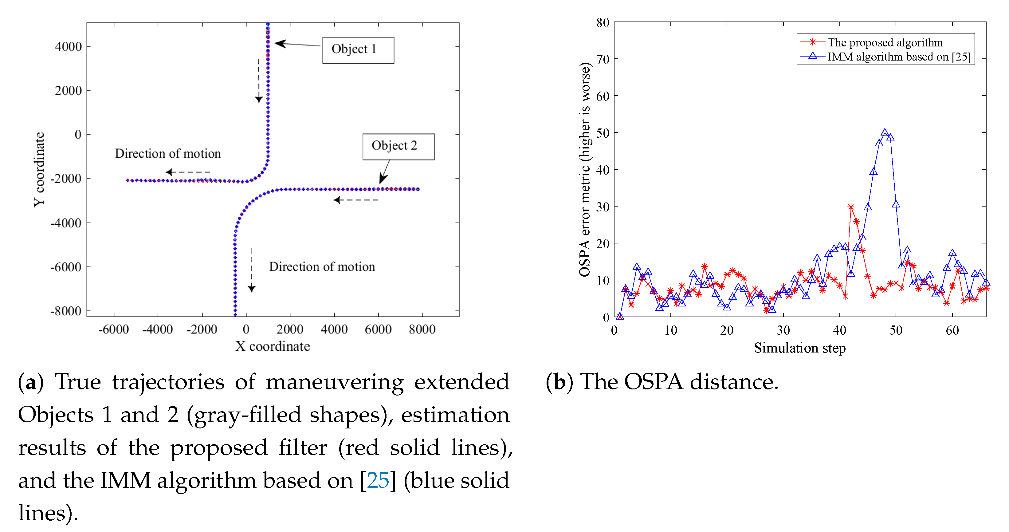
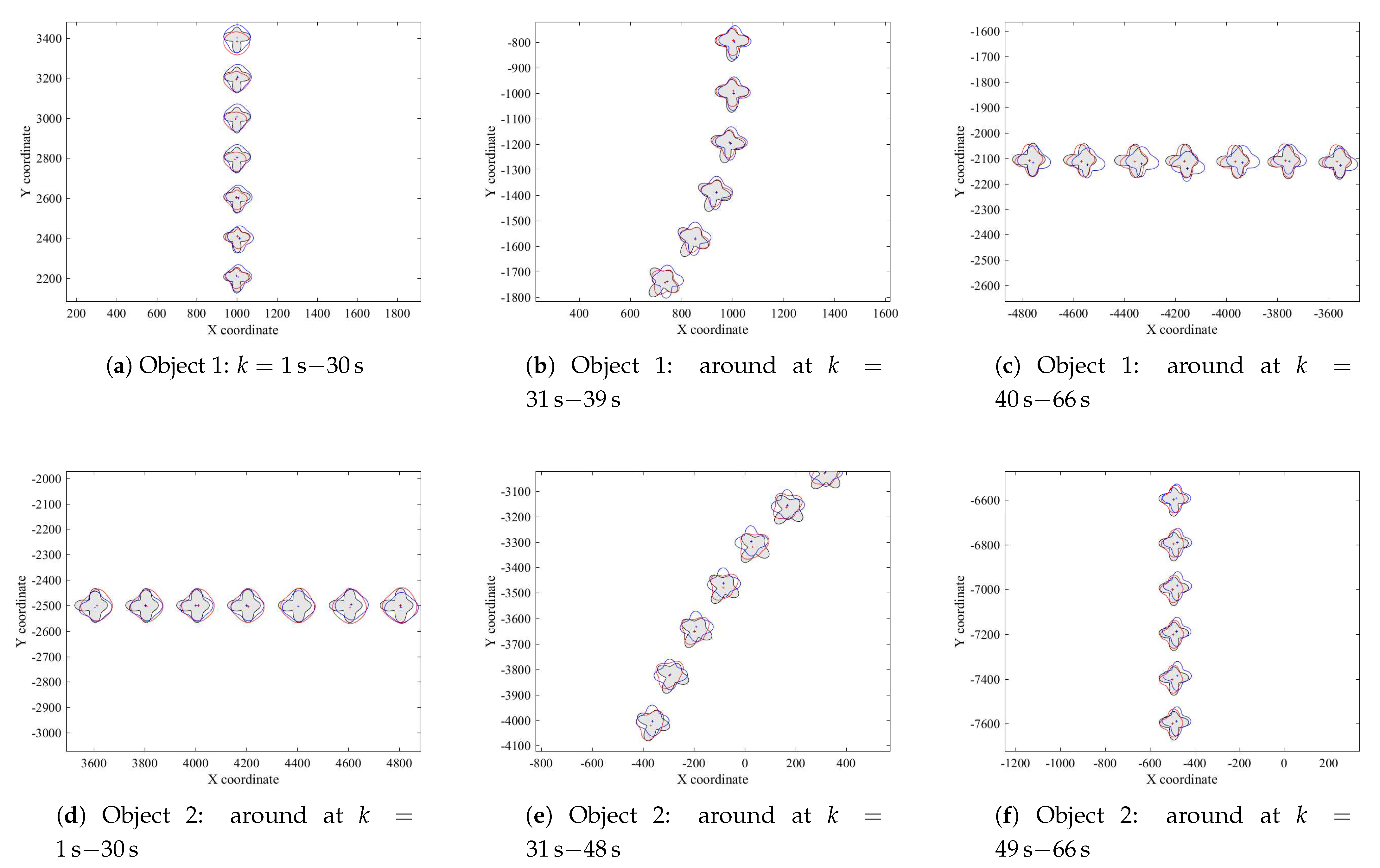
4.1. Tracking Performance in Scenario A

In this scenario, Object 1 and Object 2 are to be tracked, which started at time step k = 1 s and ended at time step k = 66 s . Object 1 and Object 2 simultaneously maneuvered with different turn rates at time step k = 31 s 39 s . The estimation results and true trajectories of these objects are shown in Figure 3a. Gray-filled shapes are true object shapes, cross symbols denote estimations of object centers, and shapes with red and blue lines are object shape estimations by the proposed filter and the IMM algorithm based on [25], respectively.
Considering that it is hard to jointly evaluate the estimation performance of object extensions, we give detailed estimated shapes of Object 1 and Object 2 in Figure 4. From Figure 4, it is evident that object extension estimations are gradually accurate in the proposed filter. Even when these objects simultaneously maneuvered, the estimation of extensions are relatively accurate. However, the IMM algorithm based on [25] has worse estimation performance in object extensions. It illustrates that the proposed maneuver models can describe different maneuvers of the star-convex objects effectively. Furthermore, they can be easily applied in this filter to obtain good estimation performance in object extensions. Moreover, Figure 4 demonstrates that the proposed merging strategy of x k , e ( j ) is reliable and capable of estimating object extensions accurately.
The estimation performance in the object number and centroid dynamics is jointly evaluated by a widely used evaluation measure known as the OSPA distance [33]. The higher the OSPA distance is, the worse the performance in the estimation of the object number and centroid positions is. From Figure 3b, the OSPA distance of the proposed filter is lower than that of the IMM algorithm based on [25]. Though the OSPA distance of the proposed filter is a little higher in the middle due to the unreasonable partitioning results of measurements, it stays low at other time steps. This implies that the proposed filter achieves more accurate estimation performance in the object number and centroid positions compared with the IMM algorithm based on [25]. This is because the proposed IMM-GMPHD filter fits well for MMSEOT to handle the complex maneuvering behaviors of star-convex extended objects.

4.2. Tracking Performance in Scenario B

In Scenario B, the star-convex extended objects to be tracked are denoted by Object 3 and Object 4, both of which started at k = 1 s and ended at k = 90 s . In this scenario, two constant left-turn motions with different turn rates (i.e., ω B ( 1 ) = 5 π 5 π 180 180 rad/s and ω B ( 2 ) = 10 π 5 π 180 180 rad/s ) and a constant velocity model with the turn rate ω B ( 3 ) = 0 rad/s are used to further test the effectiveness of the proposed filter. The initial model probabilities of these maneuver models are the same as those of Scenario A.
The true trajectories and estimation results are illustrated in Figure 5a, and the detailed estimation results of Object 3 and Object 4 are shown in Figure 6. From these figures, it can be concluded that object shape estimations are gradually close to true shapes from initial circles. When these objects maneuvered with different turn rates simultaneously, the estimation of object shapes and orientations by the proposed filter remains fairly more accurate than that of the IMM algorithm based on [25]. This demonstrates that this proposed filter can effectively handle the complex maneuvering behaviors of multiple star-convex extended objects. It also shows that the pruning and merging step in the proposed algorithm contributes to the accurate extension estimations.
Figure 5b illustrates the OSPA distance at each time step. It shows that the estimation of the object number and dynamic states by the presented filter are more accurate than that of the IMM algorithm based on [25]. In other words, the proposed IMM-GMPHD filtering recursion and the update formulas of model probabilities are effective for tracking multiple maneuvering star-convex extended objects.

4.3. Tracking Performance in Scenario C

To further validate the feasibility of the proposed filter, a complex tracking scenario (i.e., Scenario C) with crossing trajectories was chosen. In Section C, the true trajectories and estimation results of Object 5 and Object 6 are shown in Figure 7a. It can be seen that these objects crossed twice. When Object 5 and Object 6 first crossed around time step k = 23 s 30 s , their turn rates were equal to ω C ( 1 ) = 0 rad/s . When Object 5 and Object 6 crossed around time step k = 36 s 45 s , they rotated with different turn rates in different directions, i.e., Object 5 made a left-turn motion with the turn rate ω C ( 2 ) = 5 π 5 π 180 180 rad/s , while Object 6 made a right-turn motion with the turn rate ω C ( 3 ) = 5 π 5 π 180 180 rad/s .
Figure 8 gives detailed tracking results of Object 5 and Object 6. The object extension estimations by the proposed filter are ultimately close to true object shapes. When objects made turn motions or crossed, object shapes and orientations were especially more accurate compared with the IMM algorithm based on [25]. This is due to feasible maneuver models, strict and scientific update formulas of model probabilities, and the effective merging step of extension states. The estimation performance of the object number and positions is assessed by the OSPA distance in Figure 7b. The OSPA distance of the proposed filter is relatively lower than that of the IMM algorithm based on [25]. This demonstrates that the proposed filter can achieve more accurate estimation of the object number and centroid positions than the IMM algorithm based on [25]. To summarize, our filter is capable of handling complex tracking issues in MMSEOT and obtains high tracking performances in object number, centroid dynamics, and object extensions.

5. Conclusions

To deal with the unknown and time-varying maneuvering behaviors of star-convex extended objects, this paper has proposed an IMM-GMPHD filter. By integrating linear maneuver models into this filter, various turn maneuvers of objects can be described accurately from two aspects (i.e., the dynamic evolutions of both centroids and extensions). In our filter, rigorous update and merging formulas of model probabilities have been derived for dealing with the uncertainty of maneuvering models. This is the main advantage over other extended object tracking approaches. Moreover, object states have been properly merged and pruned to obtain accurate tracking results. Specifically for extension-involved states, they turned to radial functions and merged, which further improves the estimation performance of object extensions. Simulation results have verified that the proposed filter can achieve more accurate estimation performance in object number, centroid dynamics, and extensions (e.g., orientations and shapes) compared with the IMM algorithm based on [25] with original ET-GM-PHD filtering steps and RHMs. In summary, our filter may be promising for handling a large range of problems in multiple maneuvering extended object tracking.

Author Contributions

L.S. and H.Y. conceived of the idea and developed the proposed approaches. J.L. and Z.F. advised the research and helped edit the paper. Z.H. and J.P. improved the quality of the manuscript and of the completed revision. All authors have read and agreed to the published version of the manuscript.

Funding

This work was supported in part by the National Natural Science Foundation of China (U1809202), National Thirteen-Five Equipment Pre-Research Foundation of China (No. 61403120207), Aeronautical Science Foundation of China (No. 20185142003), Science and Technology Innovative Talents in Universities of Henan Province (No. 21HASTIT030), Young Backbone Teachers in Universities of Henan Province (No. 2020GGJS073), and Leading Talents of Science and Technology Innovation in the Central Plains of China (No. 194200510012).

Conflicts of Interest

The authors declare no conflict of interest.

References

  1. Zhang, L.; Mao, D.; Niu, J.; Wu, Q.M.; Ji, Y. Continuous Tracking of Targets for Stereoscopic HFSWR Based on IMM Filtering Combined with ELM. Remote Sens. 2020, 12, 272. [Google Scholar] [CrossRef] [Green Version]
  2. Zhao, M.; Zhang, X.; Yang, Q. Modified Multi-Mode Target Tracker for High-Frequency Surface Wave Radar. Remote Sens. 2018, 10, 1061. [Google Scholar] [CrossRef] [Green Version]
  3. Zhou, H.; Huang, H.; Zhao, H.; Zhao, X.; Yin, X. Adaptive Unscented Kalman Filter for Target Tracking in the Presence of Nonlinear Systems Involving Model Mismatches. Remote Sens. 2017, 9, 657. [Google Scholar] [CrossRef] [Green Version]
  4. Cheng, Y.; Yan, X.; Tang, S.; Wu, M.; Li, C. An adaptive non-zero mean damping model for trajectory tracking of hypersonic glide vehicles. Aerosp. Sci. Technol. 2021, 111, 106529. [Google Scholar] [CrossRef]
  5. Blackman, S. Multiple hypothesis tracking for multiple target tracking. IEEE Aerosp. Electr. Syst. Mag. 2004, 19, 5–18. [Google Scholar] [CrossRef]
  6. Wang, Y.; Wang, X.; Shan, Y.; Cui, N. Quantized genetic resampling particle filtering for vision-based ground moving target tracking. Aerosp. Sci. Technol. 2020, 103, 105925. [Google Scholar] [CrossRef]
  7. Mahler, R. Multitarget bayes filtering via firstorder multi target moments. IEEE Trans. Aerosp. Electr. Syst. 2003, 39, 1152–1178. [Google Scholar] [CrossRef]
  8. Mahler, R. Statistical multisource-Multitarget Information Fusion; Artech House: Norwood, MA, USA, 2007. [Google Scholar]
  9. Kim, D.; Kwon, C.; Hwang, I. Gaussian mixture probability hypothesis density filter against measurement origin uncertainty. Signal Process. 2020, 171, 107448. [Google Scholar] [CrossRef]
  10. Vo, B.N.; Singh, S.; Doucet, A. Sequential monte carlo implementation of the PHD filter for multi-target tracking. In Proceedings of the International Conference Information Fusion, 2003; pp. 792–799. Available online: http://citeseerx.ist.psu.edu/viewdoc/download;jsessionid=24BC893EC3158E28FD9689520CF57E64?doi=10.1.1.9.5930&rep=rep1&type=pdf (accessed on 24 May 2021).
  11. Clark, D.E.; Panta, K.; Vo, B.N. The GM-PHD filter multiple target tracker. In Proceedings of the 9th International Conference on Information Fusion, Florence, Italy, 10–13 July 2006; pp. 1–8. [Google Scholar]
  12. Mahler, R. CPHD and PHD filters for unknown backgrounds, II: Multitarget filtering in dynamic clutter. In Proceedings of the Sensors and Systems for Space Applications III, Orlando, FA, USA, 6 May 2009; International Society for Optics and Photonics, 2009; Volume 7330, p. 73300L. Available online: https://www.spiedigitallibrary.org/conference-proceedings-of-spie/7330/73300L/CPHD-and-PHD-filters-for-unknown-backgrounds-II--multitarget/10.1117/12.818023.full?SSO=1 (accessed on 24 May 2021).
  13. Li, P.; Ge, H.W.; Yang, J.L.; Wang, W. Modified Gaussian inverse Wishart PHD filter for tracking multiple non-ellipsoidal extended targets. Signal Process. 2018, 150, 191–203. [Google Scholar] [CrossRef]
  14. Hu, Q.; Ji, H.; Zhang, Y. A standard PHD filter for joint tracking and classification of maneuvering extended targets using random matrix. Signal Process. 2018, 144, 352–363. [Google Scholar] [CrossRef]
  15. Gilholm, K.; Salmon, D. Spatial distribution model for tracking extended objects. IEEE Proc. Radar Sonar Navig. 2005, 152, 364–371. [Google Scholar] [CrossRef]
  16. Gilholm, K.; Godsill, S.; Maskell, S.; Salmond, D. Poisson models for extended target and group tracking. In Signal and Data Processing of Small Targets; International Society for Optics and Photonics: San Diego, CA, USA, 2005; Volume 5913, p. 59130R. [Google Scholar]
  17. Mahler, R. PHD filters for nonstandard targets, I: Extended targets. In Proceedings of the IEEE 12th International Conference on Information Fusion, Seattle, WA, USA, 6–9 July 2009; pp. 915–921. [Google Scholar]
  18. Granstrom, K.; Lundquist, C.; Orguner, O. Extended target tracking using a gaussian mixture PHD filter. IEEE Trans. Aerosp. Electr. Syst. 2012, 48, 3268–3286. [Google Scholar] [CrossRef] [Green Version]
  19. Feldmann, M.; Fränken, D.; Koch, W. Tracking of extended objects and group targets using random matrices. IEEE Trans. Signal Process. 2011, 59, 1409–1420. [Google Scholar] [CrossRef]
  20. Zong, P.; Barbary, M. Improved multi-bernoulli filter for extended stealth targets tracking based on sub-random matrices. IEEE Sens. J. 2015, 16, 1428–1447. [Google Scholar] [CrossRef]
  21. Vivone, G.; Granström, K.; Braca, P.; Willett, P. Multiple sensor measurement updates for the extended target tracking random matrix model. IEEE Trans. Aerosp. Electr. Syst. 2017, 53, 2544–2558. [Google Scholar] [CrossRef]
  22. Hassan, M.; Bermak, A. Robust bayesian inference for gas identification in electronic nose applications by using random matrix theory. IEEE Sens. J. 2016, 16, 2036–2045. [Google Scholar] [CrossRef]
  23. Baum, M.; Hanebeck, U.D. Shape tracking of extended objects and group targets with star-convex RHMs. In Proceedings of the IEEE 14th International Conference on Information Fusion, Chicago, IL, USA, 5–8 July 2011; pp. 338–345. [Google Scholar]
  24. Baum, M.; Hanebeck, U.D. Extended object tracking with random hypersurface models. IEEE Trans. Aerosp. Electr. Syst. 2014, 50, 149–159. [Google Scholar] [CrossRef] [Green Version]
  25. Han, Y.; Zhu, H.; Han, C. A gaussian-mixture PHD Filter Based on random hypersurface model for multiple extended targets. In Proceedings of the IEEE Proceedings of the 16th International Conference on Information Fusion, Istanbul, Turkey, 9–12 July 2013; pp. 1752–1759. [Google Scholar]
  26. Wood, T.M. Interacting methods for manoeuvre handling in the GM-PHD filter. IEEE Trans. Aerosp. Electr. Syst. 2011, 47, 3021–3025. [Google Scholar] [CrossRef]
  27. Li, X.R.; Jilkov, V.P. Survey of maneuvering target tracking Part I: Dynamic models. IEEE Trans. Aerosp. Electr. Syst. 2003, 39, 1333–1364. [Google Scholar]
  28. Vo, B.N.; Pasha, A.; Tuan, H.D. A gaussian mixture PHD filter for nonlinear jump markov models. In Proceedings of the 45th IEEE Conference on Decision and Control, San Diego, CA, USA, 13–15 December 2006; pp. 3162–3167. [Google Scholar]
  29. Punithakumar, K.; Kirubarajan, T.; Sinha, A. Multiple-model probability hypothesis density filter for tracking maneuvering targets. IEEE Trans. Aerosp. Electr. Syst. 2008, 44, 87–98. [Google Scholar] [CrossRef]
  30. Dong, P.; Jing, Z.; Gong, D.; Tang, B. Maneuvering multi-target tracking based on variable structure multiple model GMCPHD filter. Signal Process. 2017, 141, 158–167. [Google Scholar] [CrossRef]
  31. Wang, C.; Wu, P.; He, S.; Yun, P. Robust CPHD algorithm for maneuvering targets tracking via airborne pulsed Doppler radar. Optik 2019, 178, 285–296. [Google Scholar] [CrossRef]
  32. Hirscher, T.; Scheel, A.; Reuter, S.; Dietmayer, K. Multiple extended object tracking using Gaussian processes. In Proceedings of the IEEE 19th International Conference on Information Fusion (FUSION), Heidelberg, Germany, 5–8 July 2016; pp. 868–875. [Google Scholar]
  33. Schuhmacher, D.; Vo, B.T.; Vo, B.N. A consistent metric for performance evaluation of multi-object filters. IEEE Trans. Signal Process. 2008, 56, 3447–3457. [Google Scholar] [CrossRef] [Green Version]
Figure 1. The production process of a measurement for a star-convex extended object. The shape with a dotted line is a scaled contour of a star-convex object; the shape with a solid line is the true contour of a star-convex object; the solid black spot is a measurement source; the cross symbol is a measurement.
Remotesensing 13 02963 g001
Figure 2. The complete framework of the IMM-GMPHD filter.
Remotesensing 13 02963 g002
Figure 3. Simulation results of Object 1 and Object 2 in Scenario A.
Remotesensing 13 02963 g003
Figure 4. Detailed estimations of Object 1 and Object 2 in Scenario A.
Remotesensing 13 02963 g004
Figure 5. Simulation results of Object 3 and Object 4 in Scenario B.
Remotesensing 13 02963 g005
Figure 6. Detailed estimations of Object 3 and Object 4 in Scenario B.
Remotesensing 13 02963 g006
Figure 7. Simulation results of Object 5 and Object 6 in Scenario C.
Remotesensing 13 02963 g007
Figure 8. Detailed estimations of Object 5 and Object 6 in Scenario C.
Remotesensing 13 02963 g008
Table 1. Pseudo codes for the pruning and merging step.
Input: the mixed posterior intensity D ^ k k ξ ,
each posterior intensity D i , k k ξ Z k ( i 1 , N m ),
and model probabilities corresponding to D i , k k ξ Z k .
f = 0 , I = j w ^ k k j > τ j = 1 J k k , i 1 , N m
Repeat
f = f + 1
p m = arg max w ^ i , k k j j I
U m = j I m ^ k k j m ^ k k p m T P ^ k k j 1 m ^ k k j m ^ k k p m U
merging Gaussian mixture components of the mixed posterior intensity:
w k f = j U m w ^ k k j
m m , k f = 1 w k f j U m w ^ k k j m ^ m , k k j
R m e , k f , θ = j U m R θ m ^ e , k k j N u , θ 0 , 2 π
m e , k f = leastsquare R m e , k f , θ , θ
P k f = 1 w k f j U m w ^ k k j P ^ k k j + m k f m k k j m k f m ^ k k j T
merging model probabilities:
μ i , k f = c i f j U m Λ W k j i c f
Λ W k j i = d = 1 W k j Λ d , f , k i
c f = i = 1 N m c i f Λ W k j i
merging Gaussian mixture components of each posterior intensity:
w i , k f = j U m w i , k k j
m i , m , k f = 1 w i , k f j U m w i , k k j m i , m , k k j
R m i , e , k f , θ = j U m R θ m i , e , k k j N u , θ 0 , 2 π
m i , e , k f = leastsquare R m i , e , k f , θ , θ
P i , k f = 1 w i , k f j U m w i , k k j P i , k k j + m i , k f m i , k k j m i , k f m i , k k j T
I = I \ U m
until   I =
J k = f
Output: the final mixed posterior intensity D k ξ = j = 1 J k w k j N x ; m k j , P k j ,
each posterior intensity D i , k ξ = j = 1 J k w i , k j N x ; m i , k j , P i , k j ( i 1 , N m ),
and model probabilities corresponding to D i , k ξ .
Publisher’s Note: MDPI stays neutral with regard to jurisdictional claims in published maps and institutional affiliations.

