Article

Impacts of Human Activities on the Variations in Terrestrial Water Storage of the Aral Sea Basin

1
Shaanxi Key Laboratory of Earth Surface System and Environmental Carrying Capacity, College of Urban and Environmental Sciences, Northwest University, Xi’an 710127, China
2
Institute of Earth Surface System and Hazards, College of Urban and Environmental Sciences, Northwest University, Xi’an 710127, China
3
CAS Center for Excellence in Tibetan Plateau Earth Sciences, Beijing 100101, China
*
Author to whom correspondence should be addressed.
Remote Sens. 2021, 13(15), 2923; https://doi.org/10.3390/rs13152923
Submission received: 1 June 2021 / Revised: 8 July 2021 / Accepted: 23 July 2021 / Published: 25 July 2021

Abstract

:
Assessing the impacts of human activities on the variations in terrestrial water storage (TWS) is essential for water resource management, particularly in regions like the Aral Sea Basin which suffers from severe water scarcity. In this study, the variations in TWS anomalies (TWSA) of the Aral Sea Basin during the period of April 2002 to June 2017 were analyzed using Gravity Recovery and Climate Experiment (GRACE) data and the Global Land Data Assimilation System (GLDAS) Noah model outputs. The impacts of human activities on TWS variations were further quantified through the variations in TWS components and the comparison of TWS obtained from GRACE and GLDAS. The results indicate that TWSA of the entire Aral Sea Basin derived from GRACE experienced a significant decreasing trend of 4.12 ± 1.79 mm/year (7.07 ± 3.07 km3/year) from 2002 to 2017. Trends in individual TWS components indicate that the reduction in TWS of the Aral Sea Basin was primarily attributed to surface water loss, followed by groundwater depletion, which account for ~53.16% and 11.65 ± 45.39 to 42.48 ± 54.61% of the total loss of TWS, respectively. Precipitation (P) and evapotranspiration (ET) both exhibited increasing trends, indicating that ET played a dominant role in TWS depletion from the perspective of water balance. The variations in ET and TWS induced by human activities contributed ~45.54% and ~75.24% to those in total ET and TWS of the Aral Sea Basin, respectively.

Graphical Abstract

1. Introduction

Terrestrial water storage (TWS) is an essential component of the terrestrial and global hydrological cycles, which mainly comprises surface water (lakes, rivers, and reservoirs), groundwater, soil moisture, plant canopy water, snow, and glaciers [1,2,3]. Due to the scarcity of water resources in arid and semi-arid regions, these components of TWS, particularly surface water and groundwater, become of great ecological and social importance [4,5]. In recent years, global warming has exacerbated the variability of TWS in arid and semi-arid regions, intensified further by human activities such as agricultural irrigation [6,7]. Therefore, a better understanding of the impacts of human activities on TWS variations is of great practical significance for water resource management.
The Aral Sea Basin, an endorheic basin located in arid Central Asia, suffers from severe water scarcity under the influence of human activities [8,9,10]. With the rapid increase in water withdrawal since the 1960s, especially for damming and irrigation, the eco-environment dominated by water in the Aral Sea Basin has been deteriorating [4,11,12,13]. For instance, the Aral Sea shrank sharply over the period of 1960–2018, with a reduction of 60,156.50 km2 in area and 1000.51 km3 in water volume [14]. It is thus of vital importance to assess the dynamics of TWS in this region and the impacts of human activities on TWS variations.
Traditional site observations (e.g., groundwater level and soil moisture measurements) only provide information on individual hydrological variables at point scales [15,16], and the data transparency and accessibility are often lacking; the Aral Sea Basin is no exception. The launch of the Gravity Recovery and Climate Experiment (GRACE) satellites in 2002 [17] has offered an effective technique to access the spatial and temporal variations in TWS anomalies (TWSA) [18]. The primary objective of the GRACE satellites is to monitor the Earth’s time-variable gravitational field, which reflects the mass changes mainly caused by the movement of water through the Earth’s water cycle [19]. GRACE can achieve frequent, rapid, and continuous observations at the global scale without being restricted by terrestrial conditions. GRACE satellite datasets have been widely used in numerous studies to estimate groundwater storage changes [20], regional TWS changes [21,22,23], ice sheet and glacier mass balance [24,25], and global sea level changes [26], etc.
Land surface models or hydrological models can also simulate TWS variations. Several studies theoretically estimate TWS variations (∆TWS) by using precipitation (P), evapotranspiration (ET), and total runoff (R) from these models based on the water balance equation (∆TWS = P − ET − R) [27,28], or by adding up the variations in various TWS components [15]. However, since human impacts are difficult to parameterize, most of these models can only simulate hydrological variables under natural climate conditions [29,30], and they often lack processes to simulate some important TWS components (e.g., surface water and groundwater) [6,31]. In contrast to land surface models, GRACE can detect changes in TWS caused by both natural and anthropogenic factors [32]. Therefore, the comparison of TWS derived from GRACE and land surface models can indirectly evaluate the human water withdrawal in this region.
Previous studies have focused primarily on the overall trend in TWS of the Aral Sea Basin [6,10,33,34]. However, a comprehensive and quantitative analysis of the contribution of human activities to recent TWS variations is still lacking. Therefore, in this study, we first assessed the annual and seasonal variations in TWS of the Aral Sea Basin over the period of April 2002 to June 2017, by using GRACE data and the Global Land Data Assimilation System (GLDAS) model outputs. Then, the variations in individual TWS components were calculated to indicate the impacts of human activities on TWS variations. Moreover, based on the water balance equation, P − ET obtained from GLDAS was compared with TWS from GRACE, the former of which reflects changes under natural climate conditions whereas the latter represents the total changes, to evaluate the contribution of human activities to TWS variations.

2. Materials and Methods

2.1. Study Area

The Aral Sea Basin is a vast transboundary basin in the hinterland of the Eurasian continent [35], with a spatial range of approximately 34°4′–48°40′ N, 54°56′–78°22′ E (Figure 1). It encompasses seven nations: Kazakhstan, Kyrgyzstan, Uzbekistan, Turkmenistan, Tajikistan, Afghanistan, and Iran. Topographically, the Aral Sea Basin ranges from the vast Turan Plain with the Kyzyl Kum and Kara Kum deserts in the west to the tremendous mountains of the Tien Shan and Pamirs in the east [36]. The main water resources in this region are the Amu Darya and the Syr Darya, originating from glaciers and snowfields in the Tien Shan and Pamirs, as well as the Aral Sea into which these rivers flow [9]. The Aral Sea was the world’s fourth largest inland lake in the mid-20th century, covering an area of ~68,478 km2 in 1960. However, it shrank sharply over the past six decades, and its changes caused a series of severe eco-environmental issues to the Aral Sea Basin [14,37].
The climate in the Aral Sea Basin is mostly dry–arid continental with low precipitation and high evaporation in summer, and cold and dry conditions in winter [35]. The average temperature ranges from 0 °C–4 °C in January and from 28 °C–32 °C in July. The annual precipitation varies substantially across different regions of the basin, e.g., it ranges from 80–200 mm in the valleys with the majority falling in spring and winter, 300–400 mm in the foothills, and as high as 600–800 mm on the southern and southwestern sides of the mountains. Due to the arid climate in the Aral Sea Basin, agriculture is fully dependent on a dense irrigation and drainage network, and 90% of the total water withdrawal is used for this purpose [35,38].

2.2. Data

2.2.1. GRACE Data

GRACE is a satellite mission jointly launched by the National Aeronautics and Space Administration (NASA) and the German Aerospace Center (DLR). It consists of twin satellites spaced ~220 km apart in a near-polar orbit at an altitude of ~450 km. The products of GRACE are released by the Scientific Data System composed of three major research groups: Center for Space Research (CSR), Geo-Forschungs-Zentrum (GFZ), and Jet Propulsion Laboratory (JPL). Several studies have demonstrated that spherical harmonic (SH) coefficients provided by the CSR can effectively reveal the variations in TWS, since the mass variations in atmosphere and ocean have been removed [22,39,40,41]. Therefore, the latest Release-06 (RL06) SH coefficients from the CSR were selected for this study. The data covered the period of April 2002 to June 2017, for a total of 163 months, and it was missing for 20 months (Figure 2).

2.2.2. GLDAS Data

GLDAS is a commonly used land surface modeling system, which aims to generate optimal fields of land surface states and fluxes based on satellite and ground observations, and has been frequently used in the estimation of TWS [3,42,43,44]. GLDAS derives four land surface models including Noah, Catchment (CLSM), the Community Land Model (CLM), and the Variable Infiltration Capacity (VIC) at a high spatial resolution of 1° to 0.25°. Several studies have confirmed that the Noah model exhibits a better correlation with GRACE TWS than other GLDAS models [45,46,47]. Therefore, we selected the latest GLDAS Noah Land Surface Model L4 monthly 0.25° × 0.25° V2.1 product (GLDAS_NOAH025_M_2.1) for the period of 2002–2017. The GLDAS-2.1 Noah model contains 36 variables, and 9 variables of them were selected for assessing TWS variations as well as water balance (Table 1).

2.3. Methods

2.3.1. GRACE Data Processing

The variations in TWS can be retrieved directly from GRACE SH coefficients, with the following equation applied [48]:
Δ σ θ , φ = α ρ a v e 3 l = 0 m = 0 l 2 l + 1 1 + k l P ¯ l m c o s θ × Δ C l m cos m φ + Δ S l m sin m φ
where Δ σ θ , φ represents surface mass density changes, α is the equatorial radius (the constant is 63781363.3 m), ρ a v e is the mean density of the Earth (the constant is 5517 kg/m3),   θ and φ are the geocentric latitude and longitude,   Δ C l m and Δ S l m are the SH coefficient anomalies, k l is the Loew coefficient, and P ¯ l m is the normalized Legendre function, with maximum degree l and order m expanded to 60.
The variations in TWS can also be expressed as the equivalent water height, see Equation (2), which is converted from Equation (1):
E W T θ , φ = α ρ a v e 3 ρ w a t e r l = 0 m = 0 l 2 l + 1 1 + k l P ¯ l m c o s θ × Δ C l m cos m φ + Δ S l m sin m φ
where E W T θ , φ is the equivalent water height and ρ w a t e r is the density of water (the constant is 1000 kg/m3).
According to the above principles, the following post-processing steps were performed on the SH coefficients first. The C20 terms of the SH coefficients were replaced by estimates obtained from Satellite Laster Ranging (SLR) [49]. The first-degree terms of the SH coefficients were replaced by estimates from the atmosphere and ocean models [50]. Then, a Glacial Isostatic Adjustment (GIA) correction in the model proposed by Geruo et al. [51] was applied to remove glacial rebound effects. To reduce the north–south strip error and high-frequency noise in the original data, an effective spatial filtering method is needed [52,53]. The effects of different filtering methods on retrieving TWS changes were compared, as shown in Figure 3. It can be found that TWSA without any filtering applied showed an obvious north–south strip error in space (Figure 3a), and only when Swenson destriping or Gaussian smoothing was applied, although the stripes were obviously reduced, the filtering effect was not obvious in the middle and low latitudes (Figure 3b,c). The combination of Swenson destriping and Gaussian smoothing can effectively remove the north–south strips and reveal the real information of TWSA, and the larger the Gaussian filter radius, the better the noise removal effect (Figure 3d–f). However, the real data signal will also be attenuated when the strip noise is suppressed [54], e.g., the north–south sharpening appeared when a 500 km Gaussian filter was applied (Figure 3f). Therefore, the Swenson destriping method combined with a 300 km Gaussian smoothing were selected in this study.
After the post-processing, the SH coefficients were converted into equivalent water height with a spatial resolution of 0.25° to keep consistent with the GLDAS model. The monthly TWSA was calculated from the differences between TWS in each month and the baseline average of TWS from January 2004 to December 2010, because there was no missing data in this period. In order to restore the signal reduced by truncation of the gravity coefficients and filtering, the scaling factor was then applied to GRACE TWSA over the study area [55,56]. Based on Equation (3), the scaling factor was computed by applying the same filtering method as applied to GRACE TWSA to GLDAS TWSA, and the result was 1.065.
M = i = 1 t Δ S T , i k Δ S F , i 2
where M is the objective function that we want to minimize, Δ S T , i is the unfiltered GLDAS TWSA for month i , Δ S F , i is the filtered GLDAS TWSA for month i processed in the same way as the filtered GRACE data, k is the scaling factor derived through least square regression, and t is the number of months.
In order to evaluate the uncertainty of GRACE TWSA, errors of it were calculated, which mainly include measurement error in monthly gravity field solutions and leakage error caused by truncation and filtering in the spectral domain. The measurement error was estimated as the standard deviation of the residuals of coefficients when seasonal cycles were removed [57]. The leakage error was calculated by the following equation [55]:
L e = R M S Δ S T , i k Δ S F , i R M S G R A C E R M S G L D A S
where Δ S T , i is the unfiltered GRACE TWSA for month i , Δ S F , i is the filtered GRACE TWSA for month i , k is the scaling factor, and R M S G R A C E and R M S G L D A S are the root mean square of the filtered GRACE TWSA and GLDAS TWSA, respectively.
The total errors were estimated by summing up measurement and leakage errors in quadrature, see Equation (5):
E t o t a l = M e 2 + L e 2
where E t o t a l represents the total errors, and M e and L e are the leakage error and measurement error, respectively.

2.3.2. Water Storage Equation

For an endorheic basin, the TWS changes include six major components:
∆TWS = ∆SWS + ∆GWS + ∆SMS + ∆SnWS + ∆CWS + ∆Glacier
where ∆TWS represents the total TWS changes, ∆SWS is surface water storage changes, ∆GWS is groundwater storage changes, ∆SMS is soil moisture storage changes, ∆SnWS is snow water equivalent changes, ∆CWS is plant canopy water storage changes, and ∆Glacier is glacier mass balance changes. Surface water, groundwater, and glacier mass balance are not simulated in the GLDAS Noah model, so GLDAS TWS was calculated by summing up snow water equivalent, soil moisture, and plant canopy water. The soil moisture is the sum of soil moisture in all soil profiles, including soil moisture content in 0–10 cm, 10–40 cm, 40–100 cm, and 100–200 cm underground, and root zone soil moisture. GLDAS TWSA was calculated the same way as GRACE TWSA, subtracting the average values for the period of January 2004 to December 2010 from the original data.

2.3.3. Water Balance Equation

Precipitation (P) and evapotranspiration (ET) are key components of both atmospheric and terrestrial water balances [58]. The precipitation minus evapotranspiration (P − ET) describes the net water flux into the Earth’s surface, and thus provides essential information regarding the interaction between the atmosphere and the land surface [59]. For an endorheic basin, changes in TWS (∆TWS) can be expressed as:
Δ TWS = P ET
ET is influenced by both natural climate factors and anthropogenic factors such as irrigation or groundwater pumping [30]. Since GLDAS only simulates ET under natural climate conditions, P − ET obtained from GLDAS was compared with TWS from GRACE, the former of which reflects TWS changes under natural climate conditions and the latter represents the total TWS changes, to evaluate the contribution of human activities to TWS variations.
Moreover, to quantify the impacts of human activities on the variations in ET, ET obtained from GLDAS was compared with the total ET estimated from GRACE. The total ET can be estimated as:
ET GRACE = P TWSA GRACE
where ET GRACE represents total ET and TWSA GRACE is TWSA derived from GRACE.

2.3.4. Correlation Analysis

To assess the consistency and similarity of TWSA derived from GRACE and GLDAS, Pearson’s correlation coefficient (CC) was used here, expressed as follows:
CC = i = 1 n R i R ¯ L i L ¯ i = 1 n R i R ¯ 2 i = 1 n L i L ¯ 2
where R is the monthly TWSA derived from GRACE, L is the monthly TWSA or hydro-climatic factors obtained from GLDAS, and n is the number of months.

2.3.5. Mann-Kendall Trend Test

The Mann–Kendall trend test (M–K test) is a nonparametric and robust test for accessing the significance of trends in time series data, which has been widely used in hydrological and climatic research [60,61]. In this study, the M–K test was used to detect trends of TWSA and other hydro-climatic factors.

3. Results

3.1. Variations in TWSA from GRACE

3.1.1. Temporal Variations in TWSA from GRACE

The monthly TWSA of the Aral Sea Basin retrieved by GRACE were averaged to obtain the temporal variations in TWSA during the period of April 2002 to June 2017, as shown in Figure 4a. TWSA of the Aral Sea Basin indicated a significant decreasing trend (p < 0.01) during the entire study period. The change rate of TWSA reached −4.12 ± 1.79 mm/year, equivalent to the water loss of 7.07 ± 3.07 km3/year. During the period of 2002–2005, TWSA exhibited a huge increase at a rate of 23.54 ± 0.53 mm/year (40.42 ± 0.91 km3/year), but it decreased continuously at a rate of 21.89 ± 0.36 mm/year (37.59 ± 0.61 km3/year) from 2006 to 2009, and then declined in fluctuation at a rate of 2.65 ± 4.78 mm/year (4.55 ± 8.20 km3/year) from 2010 to 2017. The maximum positive TWSA of 95.97 ± 2.07 mm appeared in May 2005, while the minimum negative TWSA of −109.10 ± 20.41 mm was observed in September 2014. The variation trend in TWSA of the Aral Sea Basin during the study period is similar to the results observed in previous studies on the Aral Sea Basin and the entirety of Central Asia (Table 2).
The year-to-year variations in monthly TWSA were also analyzed, as displayed in Figure 4b. TWSA of the Aral Sea Basin displayed dramatic seasonal variabilities, which mainly increased in spring (March–May) and decreased in other seasons, especially in autumn (September–November). The average TWSA of each month was positive from February to June, and negative from July to January, indicating that water storage of the Aral Sea Basin was surplus in the former period and deficit in the latter one. The maximum monthly average TWSA occurred in April (30.93 ± 13.59 mm) and the minimum appeared in October (−64.85 ± 6.27 mm).

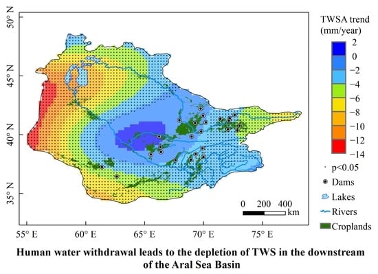
3.1.2. Spatial Variations in TWSA from GRACE

Figure 5a presents the spatial distribution of the TWSA trend in the Aral Sea Basin retrieved by GRACE during the period of April 2002 to June 2017. TWSA of the entire basin generally declined during the study period, with the spatial variation trend ranging from −12.98 to 0.66 mm/year. The variation trend in TWSA of the central Aral Sea Basin was relatively small and even exhibited a slight increase (p > 0.05). However, the significant water storage loss can be found in other areas of the basin (p < 0.05), with the largest loss in the northwest and the smallest in the southeast.
Considering that the majority of water in the Aral Sea Basin comes from cryosphere meltwater in the upstream mountains, and is consumed in the mid-downstream plains, the upstream and mid-downstream of the basin were divided according to the extent of the mountains (Figure 5b). TWSA of the two zones both indicated significant decreasing trends (p < 0.01) during the study period, with the much larger decreasing rate of 4.24 ± 1.94 mm/year in the mid-downstream and the smaller decreasing rate of 3.40 ± 0.85 mm/year in the upstream of the Aral Sea Basin (Figure 6a,b, Table 3), and their seasonal variation patterns were basically consistent with those of the entire basin (Figure 6c,d). The reduction in TWS of the upstream mountains of the Aral Sea Basin was mainly due to the melting of glaciers and snow cover. Therefore, the increase in glacier meltwater and snow water equivalent might bring more water resources to the mid-downstream plains. However, TWS in the mid-downstream of the Aral Sea Basin exhibited a tremendous decrease, especially in the downstream zone, suggesting that a large amount of water in the mid-downstream plains was utilized by human activities.

3.2. Variations in TWSA from GLDAS

TWS calculated from GLDAS includes soil moisture, snow water equivalent, and plant canopy water, which account for about 98.37%, 1.62%, and 0.01% of the total GLDAS TWS in the Aral Sea Basin, respectively. The variations in TWSA and year-to-year variations in monthly TWSA of the Aral Sea Basin from GLDAS over the study period are presented in Figure 7, and trends in TWSA, soil moisture, snow water equivalent, and plant canopy water obtained from GLDAS are listed in Table 4. The monthly GLDAS TWSA of the Aral Sea Basin ranged from −89 to 134 mm (Figure 7a), and the annual change rate of GLDAS TWSA was −0.81 mm/year (p > 0.05), equivalent to the water loss of 1.38 km3/year (Table 4). Among the components of GLDAS TWS, soil moisture anomalies increased slightly at a rate of 0.39 mm/year, snow water equivalent anomalies decreased at a rate of 1.19 mm/year, and plant canopy water anomalies remained basically unchanged (−0.01 mm/year) (Table 4). In addition, the average TWSA of each month obtained from GLDAS was positive from January to June and negative from July to December, and the maximum and minimum values were observed in April (71.79 mm) and September (−62.63 mm), respectively (Figure 7b).

3.3. Comparisons of TWSA from GRACE and GLDAS

The comparison and correlation of TWSA in the Aral Sea Basin obtained from GRACE and GLDAS over the period of April 2002 to June 2017 are presented in Figure 8. GLDAS TWSA was significantly correlated to GRACE TWSA, with a high correlation coefficient of 0.703 (p < 0.01), though the extreme values of GLDAS TWSA in some particular years were larger than those of GRACE TWSA, particularly after 2014. Both GRACE TWSA and GLDAS TWSA showed declining trends over the study period, while the declining rate of GRACE TWSA (4.12 ± 1.79 mm/year) was much larger than that of GLDAS TWSA (0.81 mm/year). Since GLDAS TWSA only reflects the variations in three elements of GRACE TWSA, these findings suggest that the variations in soil moisture, snow water equivalent, and plant canopy water account for a small proportion (~19.66%) of total TWS variations, while the variations in surface water, groundwater and glacier mass balance account for a greater one (~80.34%).

4. Discussion

In this section, the impacts of human activities on total TWS variations in the Aral Sea Basin were systematically quantified from the perspectives of TWS components (e.g., surface water and groundwater) and water balance (e.g., P and ET).

4.1. TWS Components

The excessive water consumption associated with human activities is a major component of the total water consumption in the Aral Sea Basin [62]. Around 90% of the total human water withdrawal is from irrigation, which mainly depends on surface water, and only ~3–4% comes from groundwater [9,38]. Therefore, the variations in surface water and groundwater of the Aral Sea Basin were estimated to indicate the impacts of human activities on the variations in TWS.
Based on water volume data of the Aral Sea obtained from CAWATER-info (http://www.cawater-info.net accessed on 1 October 2019) and previous study [14], the variations in water volume of the Aral Sea during the periods of 1960–2018 and 2002–2017 are presented in Figure 9a,b. Although the water volume of the Aral Sea exhibited a sharp decline during the past six decades, the declining rate has been relatively slow from 2002 to 2017 (3.75 km3/year). Given that the Aral Sea is the major component of surface water in the Aral Sea Basin, we roughly estimated the change rate of surface water in the basin using the variations in the water volume of the Aral Sea. Results indicated that surface water in the Aral Sea Basin decreased at a rate of 2.19 mm/year, accounting for ~53.16% of the declining rate of GRACE TWSA.
Glaciers in the Tien Shan and Pamirs have exhibited an overall retreat under long-term global warming [63,64]. The glacier area in the Aral Sea Basin reduced by approximately 500.85 ± 1174.72 km2 and the total loss of glacier mass ranged from 9.17 ± 12.76 to 43.89 ± 2.11 km3 w.e. over the period of 2000–2016 [14]. Based on the glacier mass loss during 2000–2016, the annual glacier mass balance of the Aral Sea Basin during 2002–2017 was estimated to be −2.74 ± 0.13 to −0.57 ± 0.80 km3 w.e./year (−1.60 ± 0.08 to −0.33 ± 0.46 mm/year), accounting for about 8.10 ± 11.27 to 38.77 ± 1.86% of the change rate of GRACE TWSA.
According to the water storage equation, the variations in the sum of surface water, groundwater, and glacier mass balance were estimated by subtracting TWSA from GRACE and GLDAS (Figure 9c). GRACE TWSA–GLDAS TWSA of the Aral Sea Basin declined intensely at a rate of 4.27 ± 1.79 mm/year, equivalent to the water loss of 7.33 ± 3.07 km3/year. Since surface water and glaciers decreased at the rates of 2.19 mm/year and 0.33 ± 0.46 to 1.60 ± 0.08 mm/year, respectively, the change rate of groundwater could be roughly estimated to be −1.75 ± 2.25 to −0.48 ± 1.87 mm/year, accounting for about 11.65 ± 45.39 to 42.48 ± 54.61% of the change rate of GRACE TWSA.
Table 5 lists trends in all TWS components of the Aral Sea Basin as well as their contributions to GRACE TWSA. The reduction in TWS of the Aral Sea Basin was primarily caused by surface water loss, followed by groundwater depletion. Other TWS components which are more affected by climate factors contributed less to TWS variations, further confirming the dominant role of human activities on TWS depletion of the Aral Sea Basin.

4.2. Water Balance

According to the water balance equation, TWS variations in endorheic basins are mainly influenced by P and ET. Human activities such as agricultural irrigation, reservoir construction, and groundwater pumping directly affect TWS through changing water loss by ET to the atmosphere [30,65]. For example, the water diversion and irrigation schemes in the Aral Sea Basin considerably increased ET, thereby reducing net water flux (P − ET) from the atmosphere to the land surface [66,67]. To quantify the water loss caused by human activities, ET and P − ET obtained from GLDAS (i.e., ETGLDAS and P − ETGLDAS) were compared with ET and TWS from GRACE (i.e., ETGRACE and GRACE TWSA), the former reflecting changes under natural climate conditions and the latter representing the total changes.
Figure 10 illustrates the variations in P, ETGRACE, ETGLDAS, and P − ETGLDAS of the Aral Sea Basin over the period of 2002–2017, and their trends are listed in Table 6. P and ETGRACE both exhibited increases at the rates of 1.36 mm/year (p > 0.01) and 4.37 ± 1.79 mm/year (p < 0.01), respectively (Figure 10a), indicating that ET was the dominant cause for the reduction in TWS of the Aral Sea Basin. ETGLDAS increased at a rate of 2.38 mm/year (p > 0.01), which accounts for ~54.46% of the increasing trend in ETGRACE, suggesting that ET induced by human activities might account for ~45.54% of the increasing trend in total ET of the Aral Sea Basin. Moreover, the decreasing rate of P − ETGLDAS (1.02 mm/year) accounts for ~24.76% of that of GRACE TWSA (Figure 10b), further suggesting that the drastic reduction in TWS of the Aral Sea Basin was more affected by human activities (~75.24%).
In summary, human activities have a profound impact on the variations in TWS of the Aral Sea Basin. TWS depletion caused by human activities contributed ~75.24% to total TWS loss of the Aral Sea Basin, which was much larger than that induced by natural climate factors. Water scarcity driven by human activities has brought great challenges to the sustainable development of economies and eco-environments in this region. It is imperative to optimize water resource management, particularly the rational utilization and protection of surface water. Otherwise, in the context of global warming, the water crisis in the Aral Sea Basin will intensify when the cryosphere meltwater weakens.

5. Conclusions

In this study, the temporal and spatial variations in TWS of the Aral Sea Basin during the period of April 2002 to June 2017 were investigated by using GRACE data and GLDAS Noah model outputs. The impacts of human activities on TWS variations were further quantified through the variations in TWS components and the comparison of TWS obtained from GRACE and GLDAS.
The results indicate that TWSA of the Aral Sea Basin derived from GRACE experienced a significant decreasing trend of 4.12 ± 1.79 mm/year from April 2002 to June 2017, equivalent to the water loss of 7.07 ± 3.07 km3/year. GRACE TWSA of the Aral Sea Basin displayed dramatic seasonal variabilities, which mainly increased in spring (March–May). The spatial heterogeneity was also observed in TWSA of the entire Aral Sea Basin: the decreasing trend in the mid-downstream (4.24 ± 1.94 mm/year) was larger than that in the upstream of the basin (3.40 ± 0.85 mm/year). GLDAS TWSA decreased at a rate of 0.81 mm/year (1.38 km3/year), which was less than that of GRACE TWSA.
The variation trends of individual TWS components indicate that the reduction in TWS of the Aral Sea Basin was primarily due to surface water loss, followed by groundwater depletion, which account for about 53.16% and 11.65 ± 45.39 to 42.48 ± 54.61% of the total loss of TWS, respectively. From the perspective of water balance, ET played a dominant role in TWS depletion of the Aral Sea Basin. The variations in ET and TWS caused by human activities contributed ~45.54% and ~75.24% to those in total ET and TWS of the Aral Sea Basin, respectively. To alleviate the water crisis in this region, it is imperative to optimize water resource management, particularly the rational utilization and protection of surface water.

Author Contributions

Conceptualization, X.Y. and N.W.; methodology, X.Y., Q.L. and A.C.; software, Y.W.; validation, Q.L.; formal analysis, X.Y. and A.C.; investigation, A.C. and Y.W.; resources, X.Y.; data curation, X.Y.; writing—original draft preparation, X.Y.; writing—review and editing, N.W., A.C., Q.L. and Y.W.; visualization, A.C.; supervision, Y.W.; project Administration, N.W.; funding acquisition, N.W. All authors have read and agreed to the published version of the manuscript.

Funding

This research was funded by the Strategic Priority Research Program of the Chinese Academy of Sciences (XDA20060201, XDA19070302), the National Key Research and Development Program of China (2017YFC0404302), and the Second Tibetan Plateau Scientific Expedition and Research Program (2019QZKK020102).

Data Availability Statement

Not applicable.

Acknowledgments

The authors are very grateful to the Center for Space Research at the University of Texas at Austin, for providing GRACE RL06 Level 2 product (ftp://podaac.jpl.nasa.gov/allData/grace/L2/CSR/RL06/ (accessed on 1 October 2019)), and the Goddard Earth Sciences Data and Information Services Center, NASA, for providing GLDAS-2.1 outputs (https://disc.gsfc.nasa.gov/datasets?keywords=GLDAS (accessed on 1 October 2019)). We appreciate the editors and the three anonymous reviewers for their valuable suggestions and advice.

Conflicts of Interest

The authors declare no conflict of interest.

References

  1. Ramillien, G.; Famiglietti, J.S.; Wahr, J. Detection of Continental Hydrology and Glaciology Signals from GRACE: A Review. Surv. Geophys. 2008, 29, 361–374. [Google Scholar] [CrossRef]
  2. Famiglietti, J.S. Remote sensing of terrestrial water storage, soil moisture and surface waters. Geophys. Monogr. Ser. 2004, 150, 197–207. [Google Scholar] [CrossRef]
  3. Nie, N.; Zhang, W.C.; Zhang, Z.J.; Guo, H.D.; Ishwaran, N. Reconstructed Terrestrial Water Storage Change (ΔTWS) from 1948 to 2012 over the Amazon Basin with the Latest GRACE and GLDAS Products. Water Resour. Manag. 2016, 30, 279–294. [Google Scholar] [CrossRef]
  4. Chen, H.; Liu, H.L.; Chen, X.; Qiao, Y.N. Analysis on impacts of hydro-climatic changes and human activities on available water changes in Central Asia. Sci. Total Environ. 2020, 737, 139779. [Google Scholar] [CrossRef] [PubMed]
  5. Deng, H.J.; Chen, Y.N. Influences of recent climate change and human activities on water storage variations in Central Asia. J. Hydrol. 2017, 544, 46–57. [Google Scholar] [CrossRef]
  6. Wang, J.D.; Song, C.Q.; Reager, J.T.; Yao, F.F.; Famiglietti, J.S.; Sheng, Y.W.; Macdonald, G.M.; Brun, F.; Schmied, H.M.; Marston, R.A.; et al. Recent global decline in endorheic basin water storages. Nat. Geosci. 2018, 11, 926–932. [Google Scholar] [CrossRef] [Green Version]
  7. Chang, L.L.; Yuan, R.Q.; Gupta, H.V.; Winter, C.L.; Niu, G.Y. Why Is the Terrestrial Water Storage in Dryland Regions Declining? A Perspective Based on Gravity Recovery and Climate Experiment Satellite Observations and Noah Land Surface Model with Multi-parameterization Schemes Model Simulations. Water Resour. Res. 2020, 56, e2020WR027102. [Google Scholar] [CrossRef]
  8. der Beek, T.A.; Voß, F.; Flörke, M. Modelling the impact of Global Change on the hydrological system of the Aral Sea basin. Phys. Chem. Earth Parts A/B/C 2011, 36, 684–695. [Google Scholar] [CrossRef]
  9. Micklin, P.; Aladin, N.V.; Plotnikov, I. The Aral Sea; Springer: Berlin/Heidelberg, Germany, 2014. [Google Scholar]
  10. Jin, Q.J.; Wei, J.F.; Yang, Z.-L.; Lin, P.R. Irrigation-induced environmental changes around the Aral Sea: An integrated view from multiple satellite observations. Remote Sens. 2017, 9, 900. [Google Scholar] [CrossRef] [Green Version]
  11. Micklin, P. The Aral Sea disaster. Annu. Rev. Earth Planet. Sci. 2007, 35, 47–72. [Google Scholar] [CrossRef] [Green Version]
  12. Wang, X.X.; Chen, Y.N.; Li, Z.; Fang, G.H.; Wang, F.; Liu, H.J. The impact of climate change and human activities on the Aral Sea Basin over the past 50 years. Atmos. Res. 2020, 245, 105125. [Google Scholar] [CrossRef]
  13. Huang, W.J.; Duan, W.L.; Chen, Y.N. Rapidly declining surface and terrestrial water resources in Central Asia driven by socio-economic and climatic changes. Sci. Total Environ. 2021, 784, 147193. [Google Scholar] [CrossRef]
  14. Yang, X.W.; Wang, N.L.; Chen, A.A.; He, J.; Hua, T.; Qie, Y.F. Changes in area and water volume of the Aral Sea in the arid Central Asia over the period of 1960–2018 and their causes. Catena 2020, 191, 104566. [Google Scholar] [CrossRef]
  15. Jing, W.L.; Zhao, X.D.; Yao, L.; Jiang, H.; Xu, J.H.; Yang, J.; Li, Y. Variations in terrestrial water storage in the Lancang-Mekong river basin from GRACE solutions and land surface model. J. Hydrol. 2020, 580, 124258. [Google Scholar] [CrossRef]
  16. Hu, W.J.; Liu, H.L.; Bao, A.M.; Attia, M.E. Influences of environmental changes on water storage variations in Central Asia. J. Geogr. Sci. 2018, 28, 985–1000. [Google Scholar] [CrossRef] [Green Version]
  17. Tapley, B.D.; Bettadpur, S.; Ries, J.C.; Thompson, P.F.; Watkins, M.M. GRACE Measurements of Mass Variability in the Earth System. Science 2004, 305, 503–505. [Google Scholar] [CrossRef] [Green Version]
  18. Wahr, J.; Swenson, S.; Zlotnicki, V.; Velicogna, I. Time-variable gravity from GRACE: First results. Geophys. Res. Lett. 2004, 31, L11501. [Google Scholar] [CrossRef] [Green Version]
  19. Scanlon, B.R.; Zhang, Z.Z.; Save, H.; Wiese, D.N.; Landerer, F.W.; Long, D.; Longuevergne, L.; Chen, J.L. Global evaluation of new GRACE mascon products for hydrologic applications. Water Resour. Res. 2016, 52, 9412–9429. [Google Scholar] [CrossRef]
  20. Yin, W.J.; Li, T.Q.; Zheng, W.; Han, S.-C.; Hu, L.T.; Tangdamrongsub, N.; Šprlák, M.; Huang, Z.Y. Improving regional groundwater storage estimates from GRACE and global hydrological models over Tasmania, Australia. Hydrogeol. J. 2020, 28, 1809–1825. [Google Scholar] [CrossRef]
  21. Khandu, K.; Forootan, E.; Schumacher, M.; Awange, J.L.; Schmied, H.M. Exploring the influence of precipitation extremes and human water use on total water storage (TWS) changes in the Ganges-Brahmaputra-Meghna River Basin. Water Resour. Res. 2016, 52, 2240–2258. [Google Scholar] [CrossRef] [Green Version]
  22. Shamsudduha, M.; Taylor, R.G.; Jones, D.; Longuevergne, L.; Owor, M.; Tindimugaya, C. Recent changes in terrestrial water storage in the Upper Nile Basin: An evaluation of commonly used gridded GRACE products. Hydrol. Earth Syst. Sci. 2017, 21, 4533–4549. [Google Scholar] [CrossRef] [Green Version]
  23. Deng, H.G.; Pepin, N.C.; Liu, Q.; Chen, Y.N. Understanding the spatial differences in terrestrial water storage variations in the Tibetan Plateau from 2002 to 2016. Clim. Chang. 2018, 151, 379–393. [Google Scholar] [CrossRef] [Green Version]
  24. Ciracì, E.; Velicogna, I.; Swenson, S. Continuity of the Mass Loss of the World’s Glaciers and Ice Caps from the GRACE and GRACE Follow-On Missions. Geophys. Res. Lett. 2020, 47, e2019GL086926. [Google Scholar] [CrossRef]
  25. Ghobadi-Far, K.; Šprlák, M.; Han, S.-C. Determination of ellipsoidal surface mass change from GRACE time-variable gravity data. Geophys. J. Int. 2019, 219, 248–259. [Google Scholar] [CrossRef]
  26. Tapley, B.D.; Watkins, M.M.; Flechtner, F.; Reigber, C.; Bettadpur, S.; Rodell, M.; Sasgen, I.; Famiglietti, J.S.; Landerer, F.W.; Chambers, D.P.; et al. Contributions of GRACE to understanding climate change. Nat. Clim. Chang. 2019, 9, 358–369. [Google Scholar] [CrossRef]
  27. Soni, A.; Syed, T.H. Analysis of variations and controls of evapotranspiration over major Indian River Basins (1982–2014). Sci. Total Environ. 2021, 754, 141892. [Google Scholar] [CrossRef]
  28. Zeng, N.; Yoon, J.-H.; Mariotti, A.; Swenson, S. Variability of basin-scale terrestrial water storage from a PER water budget method: The Amazon and the Mississippi. J. Clim. 2008, 21, 248–265. [Google Scholar] [CrossRef]
  29. Pokhrel, Y.N.; Koirala, S.; Yeh, P.J.-F.; Hanasaki, N.; Longuevergne, L.; Kanae, S.; Oki, T. Incorporation of groundwater pumping in a global Land Surface Model with the representation of human impacts. Water Resour. Res. 2015, 51, 78–96. [Google Scholar] [CrossRef] [Green Version]
  30. Pan, Y.; Zhang, C.; Gong, H.L.; Yeh, P.J.-F.; Shen, Y.J.; Guo, Y.; Huang, Z.Y.; Li, X.J. Detection of human-induced evapotranspiration using GRACE satellite observations in the Haihe River basin of China. Geophys. Res. Lett. 2017, 44, 190–199. [Google Scholar] [CrossRef]
  31. Long, D.; Longuevergne, L.; Scanlon, B.R. Global analysis of approaches for deriving total water storage changes from GRACE satellites. Water Resour. Res. 2015, 51, 2574–2594. [Google Scholar] [CrossRef] [Green Version]
  32. Tangdamrongsub, N.; Han, S.-C.; Jasinski, M.F.; Šprlák, M. Quantifying water storage change and land subsidence induced by reservoir impoundment using GRACE, Landsat, and GPS data. Remote Sens. Environ. 2019, 233, 111385. [Google Scholar] [CrossRef]
  33. Tao, D.L.; Shi, H.L.; Gao, C.C.; Zhan, J.G.; Ke, X.P. Water Storage Monitoring in the Aral Sea and its Endorheic Basin from Multi-satellite Data and a Hydrological Model. Remote Sens. 2020, 12, 2408. [Google Scholar] [CrossRef]
  34. Hu, Z.Y.; Zhang, Z.Z.; Sang, Y.-F.; Qian, J.; Feng, W.; Chen, X.; Zhou, Q.M. Temporal and spatial variations in the terrestrial water storage across Central Asia based on multiple satellite datasets and global hydrological models. J. Hydrol. 2021, 596, 126013. [Google Scholar] [CrossRef]
  35. Löw, F.; Prishchepov, A.V.; Waldner, F.; Dubovyk, O.; Akramkhanov, A.; Biradar, C.; Lamers, J.P.A. Mapping Cropland abandonment in the Aral Sea Basin with MODIS time series. Remote Sens. 2018, 10, 159. [Google Scholar] [CrossRef] [Green Version]
  36. Conrad, C.; Schönbrodt-Stitt, S.; Löw, F.; Sorokin, D.; Paeth, H. Cropping Intensity in the Aral Sea Basin and Its Dependency from the Runoff Formation 2000–2012. Remote Sens. 2016, 8, 630. [Google Scholar] [CrossRef] [Green Version]
  37. Micklin, P. The future Aral Sea: Hope and despair. Environ. Earth Sci. 2016, 75, 844. [Google Scholar] [CrossRef]
  38. Bekchanov, M.; Ringler, C.; Bhaduri, A.; Jeuland, M. Optimizing irrigation efficiency improvements in the Aral Sea Basin. Water Resour. Econ. 2016, 13, 30–45. [Google Scholar] [CrossRef]
  39. Xavier, L.; Becker, M.; Cazenave, A.; Longuevergne, L.; LloveL, W.; Filho, O.R. Interannual variability in water storage over 2003–2007 in the Amazon Basin from GRACE space gravimetry, in situ river level and precipitation data. Remote Sens. Environ. 2010, 114, 1629–1637. [Google Scholar] [CrossRef] [Green Version]
  40. Feng, W. GRAMAT: A comprehensive Matlab toolbox for estimating global mass variations from GRACE satellite data. Earth Sci. Inform. 2019, 12, 389–404. [Google Scholar] [CrossRef]
  41. Tangdamrongsub, N.; Šprlák, M. The Assessment of Hydrologic- and Flood-Induced Land Deformation in Data-Sparse Regions Using GRACE/GRACE-FO Data Assimilation. Remote Sens. 2021, 13, 235. [Google Scholar] [CrossRef]
  42. Rodell, M.; Houser, P.R.; Jambor, U.; Gottschalck, J.; Mitchell, K.; Meng, C.-J.; Arsenault, K.; Cosgrove, B.; Radakovich, J.; Bosilovich, M.; et al. The global land data assimilation system. Bull. Am. Meteorol. Soc. 2004, 85, 381–394. [Google Scholar] [CrossRef] [Green Version]
  43. Syed, T.H.; Famiglietti, J.S.; Rodell, M.; Chen, J.L.; Wilson, C.R. Analysis of terrestrial water storage changes from GRACE and GLDAS. Water Resour. Res. 2008, 44, W02433. [Google Scholar] [CrossRef]
  44. Hsu, Y.-J.; Fu, Y.N.; Bürgmann, R.; Hsu, S.-Y.; Lin, C.-C.; Tang, C.-H.; Wu, Y.-M. Assessing seasonal and interannual water storage variations in Taiwan using geodetic and hydrological data. Earth Planet. Sci. Lett. 2020, 550, 116532. [Google Scholar] [CrossRef]
  45. Yang, T.; Wang, C.; Yu, Z.B.; Xu, F. Characterization of spatio-temporal patterns for various GRACE- and GLDAS-born estimates for changes of global terrestrial water storage. Glob. Planet. Chang. 2013, 109, 30–37. [Google Scholar] [CrossRef]
  46. Grippa, M.; Kergoat, L.; Frappart, F.; Araud, Q.; Boone, A.; de Rosnay, P.; Lemoine, J.-M.; Gascoin, S.; Balsamo, G.; Ottle, C.; et al. Land water storage variability over West Africa estimated by Gravity Recovery and Climate Experiment (GRACE) and land surface models. Water Resour. Res. 2011, 47, W05549. [Google Scholar] [CrossRef]
  47. Wang, L.S.; Chen, C.; Thomas, M.; Kaban, M.K.; Güntner, A.; Du, J.S. Increased water storage of Lake Qinghai during 2004–2012 from GRACE data, hydrological models, radar altimetry and in situ measurements. Geophys. J. Int. 2018, 212, 679–693. [Google Scholar] [CrossRef]
  48. Swenson, S.C.; Wahr, J.M. Methods for inferring regional surface-mass anomalies from Gravity Recovery and Climate Experiment (GRACE) measurements of time-variable gravity. J. Geophys. Res. Solid Earth 2002, 107, 2193. [Google Scholar] [CrossRef] [Green Version]
  49. Cheng, M.K.; Tapley, B.D. Variations in the Earth’s oblateness during the past 28 years. J. Geophys. Res. Solid Earth 2004, 109, B03406. [Google Scholar] [CrossRef]
  50. Swenson, S.; Chambers, D.P.; Wahr, J. Estimating geocenter variations from a combination of GRACE and ocean model output. J. Geophys. Res. Solid Earth 2008, 113, B08410. [Google Scholar] [CrossRef] [Green Version]
  51. Geruo, A.; Wahr, J.M.; Zhong, S.J. Computations of the viscoelastic response of a 3-D compressible Earth to surface loading: An application to Glacial Isostatic Adjustment in Antarctica and Canada. Geophys. J. Int. 2013, 192, 557–572. [Google Scholar] [CrossRef]
  52. Swenson, S.; Wahr, J. Post-processing removal of correlated errors in GRACE data. Geophys. Res. Lett. 2006, 33, L08402. [Google Scholar] [CrossRef]
  53. Wahr, J.; Molenaar, M.; Bryan, F. Time variability of the Earth’s gravity field: Hydrological and oceanic effects and their possible detection using GRACE. J. Geophys. Res. Solid Earth 1998, 103, 30205–30229. [Google Scholar] [CrossRef]
  54. Werth, S.; Schmidt, R.; Kusche, J.; Güntner, A. Evaluation of GRACE filter tools from a hydrological perspective. Geophys. J. Int. 2010, 179, 1499–1515. [Google Scholar] [CrossRef] [Green Version]
  55. Landerer, F.W.; Swenson, S.C. Accuracy of scaled GRACE terrestrial water storage estimates. Water Resour. Res. 2012, 48, W04531. [Google Scholar] [CrossRef]
  56. Famiglietti, J.S.; Lo, M.; Ho, S.L.; Bethune, J.; Anderson, K.J.; Syed, T.H.; Swenson, S.C.; Linage, C.R.D.; Rodell, M. Satellites measure recent rates of groundwater depletion in California’s Central Valley. Geophys. Res. Lett. 2011, 38, L03403. [Google Scholar] [CrossRef] [Green Version]
  57. Wahr, J.; Swenson, S.; Velicogna, I. The accuracy of GRACE mass estimates. Geophys. Res. Lett. 2006, 33, L06401. [Google Scholar] [CrossRef] [Green Version]
  58. Meng, F.C.; Su, F.G.; Li, Y.; Tong, K. Changes in terrestrial water storage during 2003–2014 and possible causes in Tibetan Plateau. J. Geophys. Res. Atmos. 2019, 124, 2909–2931. [Google Scholar] [CrossRef]
  59. Swenson, S.; Wahr, J. Estimating Large-Scale Precipitation Minus Evapotranspiration from GRACE Satellite Gravity Measurements. J. Hydrometeorol. 2006, 7, 252–269. [Google Scholar] [CrossRef] [Green Version]
  60. Hamed, K.H. Trend detection in hydrologic data: The Mann–Kendall trend test under the scaling hypothesis. J. Hydrol. 2008, 349, 350–363. [Google Scholar] [CrossRef]
  61. Shadmani, M.; Marofi, S.; Roknian, M. Trend Analysis in Reference Evapotranspiration Using Mann-Kendall and Spearman’s Rho Tests in Arid Regions of Iran. Water Resour. Manag. 2012, 26, 211–224. [Google Scholar] [CrossRef] [Green Version]
  62. Kostianoy, A.G.; Kosarev, A.N. The Aral Sea Environment; Springer: Berlin/Heidelberg, Germany, 2010. [Google Scholar]
  63. Dehecq, A.; Gourmelen, N.; Gardner, A.S.; Brun, F.; Goldberg, D.; Nienow, P.W.; Berthier, E.; Vincent, C.; Wagnon, P.; Trouvé, E. Twenty-first century glacier slowdown driven by mass loss in High Mountain Asia. Nat. Geosci. 2019, 12, 22–27. [Google Scholar] [CrossRef]
  64. Brun, F.; Berthier, E.; Wagnon, P.; Kääb, A.; Treichler, D. A spatially resolved estimate of High Mountain Asia glacier mass balances from 2000 to 2016. Nat. Geosci. 2017, 10, 668–673. [Google Scholar] [CrossRef] [PubMed]
  65. Destouni, G.; Jaramillo, F.; Prieto, C. Hydroclimatic shifts driven by human water use for food and energy production. Nat. Clim. Chang. 2013, 3, 213–217. [Google Scholar] [CrossRef]
  66. Shibuo, Y.; Jarsjö, J.; Destouni, G. Hydrological responses to climate change and irrigation in the Aral Sea drainage basin. Geophys. Res. Lett. 2007, 34, L21406. [Google Scholar] [CrossRef]
  67. Destouni, G.; Asokan, S.M.; Jarsjö, J. Inland hydro-climatic interaction: Effects of human water use on regional climate. Geophys. Res. Lett. 2010, 37, L18402. [Google Scholar] [CrossRef]
Figure 1. Land-use map of the Aral Sea Basin for the year 2002. The land-cover data were from the MODIS MCD12Q1 product, glacier data were derived from the Randolph Glacier Inventory (RGI) 6.0, and dam data were obtained from the Global Reservoir and Dam Database (GRanD).
Remotesensing 13 02923 g001
Figure 2. Time distribution and availability of the GRACE data.
Remotesensing 13 02923 g002
Figure 3. The spatial pattern of global TWSA obtained from GRACE in April 2002, with no filtering applied (a), only Swenson destriping applied (b), only 300 km Gaussian smoothing applied (c), and a combination of Swenson destriping and 200 km (d), 300 km (e), and 500 km (f) Gaussian smoothing applied.
Remotesensing 13 02923 g003
Figure 4. The variations in TWSA and precipitation (a), and year-to-year variations in monthly TWSA (b) of the Aral Sea Basin during the period of April 2002 to June 2017. In (a), the blue bars represent the data uncertainty. In (b), the red horizontal lines represent the month’s median TWSA, the blue dots represent the month’s average TWSA, the boxes represent the inner-quartile range, and the whiskers represent the full range of the data.
Remotesensing 13 02923 g004
Figure 5. The spatial variation trend in TWSA of the Aral Sea Basin retrieved by GRACE during the period of April 2002 to June 2017 (a), and the distribution of the upstream (I) and mid-downstream (II) of the Aral Sea Basin (b).
Remotesensing 13 02923 g005
Figure 6. The variations in TWSA and precipitation of the upstream (a) and mid-downstream (b) of the Aral Sea Basin, and the year-to-year variations in monthly TWSA of the upstream (c) and mid-downstream (d) of the Aral Sea Basin from April 2002 to June 2017. In (a,b), the blue bars represent the data uncertainty. In (c,d), the red horizontal lines represent the month’s median TWSA, the blue dots represent the month’s average TWSA, the boxes represent the inner-quartile range, and the whiskers represent the full range of the data.
Remotesensing 13 02923 g006
Figure 7. The variations in TWSA (a) and year-to-year variations in monthly TWSA (b) of the Aral Sea Basin from GLDAS during the period of April 2002 to June 2017. In (b), the red horizontal lines represent the month’s median TWSA, the blue dots represent the month’s average TWSA, the boxes represent the inner-quartile range, and the whiskers represent the full range of the data.
Remotesensing 13 02923 g007
Figure 8. The comparison (a) and correlation (b) between GRACE TWSA and GLDAS TWSA in the Aral Sea Basin. The blue bars represent the data uncertainty.
Remotesensing 13 02923 g008
Figure 9. Variations in water volume of the Aral Sea during the periods of 1960–2018 (a) and 2002–2017 (b), variations in GRACE TWSA–GLDAS TWSA of the Aral Sea Basin during 2002–2017 (c), and the comparison of GRACE TWSA and GRACE TWSA–GLDAS TWSA (d). The blue bars represent the data uncertainty.
Remotesensing 13 02923 g009
Figure 10. The variations in P, ETGRACE, ETGLDAS (a), P − ETGLDAS, and GRACE TWSA (b) of the Aral Sea Basin over the period of 2002–2017. The black bars represent the data uncertainty.
Remotesensing 13 02923 g010
Table 1. GLDAS variables used in this study.
Short NameDescriptionUnits
SoilMoi0_10cm_instSoil moisture content (0–10 cm underground)kg m−2
SoilMoi10_40cm_instSoil moisture content (10–40 cm underground)kg m−2
SoilMoi40_100cm_instSoil moisture content (40–100 cm underground)kg m−2
SoilMoi100_200cm_instSoil moisture content (100–200 cm underground)kg m−2
RootMoist_instRoot zone soil moisturekg m−2
CanopInt_instPlant canopy surface waterkg m−2
SWE_instSnow depth water equivalentkg m−2
Rainf_f_tavgTotal precipitation ratekg m−2 s−1
Evap_tavgEvapotranspirationkg m−2 s−1
Table 2. Comparisons of the variation trend in TWSA of the Aral Sea Basin with the results observed in previous studies.
RegionsTime RangesTrendsSources
mm/yearkm3/year
Aral Sea Basin2002–2016−7.31 ± 1.68Wang et al. [6]
Aral Sea Basin2003–2017−5.85 ± 2.25Tao et al. [33]
Central Asia2003–2014−4.74Hu et al. [34]
Central Asia2003–2013−4.44 ± 2.2Deng and Chen [5]
Aral Sea Basin2002–2017−4.12 ± 1.79−7.07 ± 3.07This study
Table 3. Trends in TWSA of the Aral Sea Basin and the typical zones derived from GRACE.
RegionsTrendsp-Value
mm/yearkm3/year
Aral Sea Basin−4.12 ± 1.79−7.07 ± 3.070.000
Upstream of the Aral Sea Basin−3.40 ± 0.85−0.93 ± 0.230.002
Mid-downstream of the Aral Sea Basin−4.24 ± 1.94−6.12 ± 2.810.000
Table 4. Trends in TWSA, soil moisture, snow water equivalent, and plant canopy water of the Aral Sea Basin from GLDAS.
VariablesTrendsp-Value
mm/yearkm3/year
GLDAS TWSA−0.81−1.380.949
Soil moisture anomalies0.390.680.956
Snow water equivalent anomalies−1.19−2.050.472
Plant canopy water anomalies−0.01−0.010.259
Table 5. Trends in soil moisture, snow water equivalent, plant canopy water, glacier mass balance, surface water, and groundwater, and their contributions to GRACE TWSA during 2002–2017.
VariablesTrendsContributions (%) to TWSA
mm/yearkm3/year
Soil moisture anomalies0.390.68−9.47%
Snow water equivalent anomalies−1.19−2.0528.88%
Plant canopy water anomalies−0.01−0.010.24%
Glacier mass balance−1.60 ± 0.08~−0.33 ± 0.46−2.74 ± 0.13~−0.57 ± 0.808.10 ± 11.27~38.77 ± 1.86%
Surface water−2.19−3.7553.16%
Groundwater−1.75 ± 2.25~−0.48 ± 1.87−3.01 ± 3.87~−0.84 ± 3.2011.65 ± 45.39~42.48 ± 54.61%
GRACE TWSA−4.12 ± 1.79−7.07 ± 3.07
Table 6. Trends in P, ETGRACE, ETGLDAS, P − ETGLDAS, and GRACE TWSA of the Aral Sea Basin during the period of 2002–2017.
VariablesTrendsp-Value
mm/yearkm3/year
P1.362.340.627
ETGRACE4.37 ± 1.797.50 ± 3.070.000
ETGLDAS2.384.090.137
P − ETGLDAS−1.02−1.750.505
GRACE TWSA−4.12 ± 1.79−7.07 ± 3.070.000
Publisher’s Note: MDPI stays neutral with regard to jurisdictional claims in published maps and institutional affiliations.

