Article

Supercooled Liquid Water Detection Capabilities from Ka-Band Doppler Profiling Radars: Moment-Based Algorithm Formulation and Assessment

by
Petros Kalogeras
1,2,*,
Alessandro Battaglia
1,2,3 and
Pavlos Kollias
4,5
1
Department of Physics and Astronomy, University of Leicester, Leicester LE1 7RH, UK
2
National Centre for Earth Observation, Leicester LE4 5SP, UK
3
DIATI, Politecnico di Torino, 10129 Turin, Italy
4
Department of Environmental and Climate Sciences, Brookhaven National Laboratory, Upton, NY 11973, USA
5
Division of Atmospheric Sciences, Stony Brook University, Stony Brook, NY 11794, USA
*
Author to whom correspondence should be addressed.
Remote Sens. 2021, 13(15), 2891; https://doi.org/10.3390/rs13152891
Submission received: 24 June 2021 / Revised: 19 July 2021 / Accepted: 19 July 2021 / Published: 23 July 2021
(This article belongs to the Special Issue Radar Remote Sensing of Cloud and Precipitation)

Abstract

:
The occurrence of supercooled liquid water in mixed-phase cloud (MPC) affects their cloud microphysical and radiative properties. The prevalence of MPCs in the mid- and high latitudes translates these effects to significant contributions to Earth’s radiative balance and hydrological cycle. The current study develops and assesses a radar-only, moment-based phase partition technique for the demarcation of supercooled liquid water volumes in arctic, MPC conditions. The study utilizes observations from the Ka band profiling radar, the collocated high spectral resolution lidar, and ambient temperature profiles from radio sounding deployments following a statistical analysis of 5.5 years of data (January 2014–May 2019) from the Atmospheric Radiation Measurement observatory at the North Slope of Alaska. The ice/liquid phase partition occurs via a per-pixel, neighborhood-dependent algorithm based on the premise that the partitioning can be deduced by examining the mean values of locally sampled probability distributions of radar-based observables and then compare those against the means of climatologically derived, per-phase probability distributions. Analyzed radar observables include linear depolarization ratio (LDR), spectral width, and vertical gradients of reflectivity factor and radial velocity corrected for vertical air motion. Results highlight that the optimal supercooled liquid water detection skill levels are realized for the radar variable combination of spectral width and reflectivity vertical gradient, suggesting that radar-based polarimetry, in the absence of full LDR spectra, is not as critical as Doppler capabilities. The cloud phase masking technique is proven particularly reliable when applied to cloud tops with an Equitable Threat Score (ETS) of 65%; the detection of embedded supercooled layers remains much more uncertain (ETS = 27%).

1. Introduction

The phase of hydrometeors in cloud and precipitation systems is broadly classified as liquid, ice, and mixed-phase. Above melting point (T d r y > 0 ° C) clouds are composed only of liquid hydrometeors, while at low temperatures (T d r y < 38 ° C) only ice phase hydrometeors are present. Mixed-phase cloud (MPC) conditions can appear for ambient temperatures T d r y [ 38 , 0 ] ° C, in which case clouds may contain either one of the previous two phases or a mixture of both [1]. It is under those conditions that non-frozen liquid water appears in a metastable thermodynamic state that is referred to as supercooled liquid water (SLW). SLW has been observed worldwide in conditions of varied dynamics ranging from stratiform to convective, within the arctic, in mid-latitudes or the tropics [2,3,4,5,6]. The complex interplay between all three phases renders the study of mixed-phase processes more challenging; yet, because the microscopic and macroscopic cloud characteristics that dictate both its radiative properties and evolution are appreciably affected by its phase, their better understanding remains of focal interest for Earth’s energy budget studies [7,8], the formation and evolution of global weather patterns [9], and climate feedback mechanisms [10,11]. The radiative properties are impacted because liquid and solid hydrometeors have dissimilar scattering and absorption electromagnetic cross sections across the electromagnetic spectrum. Moreover, emission by low-level SLW clouds also enhances near-surface melting [12,13]. Considering the occurrence of SLW-bearing clouds worldwide [14], a better mixed-phase cloud representation in climate modeling, climate sensitivity, and radiative forcing studies (as seen in [15,16,17]) is essential.
For the advancement of the understanding of MPC processes, a wide array of observational setups has been deployed that involves in situ observations [3,18], ground-based remote sensing [19,20] and the methods highlighted therein), or spaceborne observations [21,22]. Applied techniques, whether ground-based or spaceborne, typically rely on multiple sensors (active and passive), exploiting instrumentation complementarities for cross-validation. Examples of the more commonly deployed sensors include millimeter cloud radar systems (MMCR), ceilometers, microwave radiometers, and radiosondes, although the depolarization lidar usually resides at the heart of phase discrimination methods. This is due to the lidar capability in separating liquid from ice thanks to its high backscatter and low depolarization [23,24,25]. However, lidar operating wavelengths (visible to near-infrared) render those sensors susceptible to signal extinction in the presence of liquid water or optically thicker ice, thereby reducing their overall potential for cloud observations as opposed to MMCRs for which atmospheric attenuation at 35–100 GHz is not as prohibitive. Hydrometeor classification in mixed-phase conditions has been conducted in terms of (i) neural networks [26], (ii) fuzzy logic implementations [27], (iii) multi-sensor applications [28,29], and (iv) radar-only [30,31] by analyzing Doppler spectra morphological features. Doppler cloud radars [32] have demonstrated potential in SLW detection capabilities by radar-only means in arctic, mixed-phase scenes in that cloud-top-condensing liquid water appears more detectable than liquid being embedded-in-ice based on statistical characteristics (radar observables’ distribution parameters) of each cloud class when compared to ice cloudy volumes.
Despite limitations that arise from the absence of instrumentation complementarities, single-frequency phase discrimination methodologies have not been fully explored. This study constitutes an effort to formulate a radar-only, moment-based technique for the detection of SLW volumes in arctic, mixed-phase conditions by exploring not only point-wise radar observables but also radar-based variables that account for volumetric growth and sedimentation variation with altitude within localized time-height neighborhoods. Radar observables under examination follow from the time-height patterns of linear depolarization ratio ( L D R ), spectral width ( σ v ), and vertical gradients (denoted z ) of measured radar reflectivity factor (Z) and Mean Doppler velocity ( M D V ) corrected for vertical air motion (designated as sedimentation velocity, S D V ). The radar-based fields L D R , z Z , and z S D V are selected under the premise that SLW droplets have dissimilar microphysical characteristics (mass density and shape) and vertical growth evolution when compared against ice-only cloudy volumes. Additionally, phase-transition regimes can potentially be demarcated from those of sedimenting ice by examining the radial velocity-uniformity in terms of spectral width. The current document demonstrates, implements, and assesses the applicability in an ice/liquid phase partition scheme of the smaller L D R yet greater σ v , z Z , and z S D V that are more likely to be encountered in condensation regimes of said mixed-phase conditions. Thereby, the need to examine either full radar-based MDV or LDR spectra (as seen in [30,31,33,34]) or any depolarization lidar-based variables, can be bypassed.
The paper is structured as follows. Section 2 outlines the employed dataset and observing systems. Section 3 provides auxiliary climatological features of the observed mixed-phase scenes for the North Slope of Alaska ARM site. Section 4 explicates via a characteristic case study the basis and rationale for selecting certain radar-based variables the technique in demonstration relies on. The analysis proceeds to Section 5 where the method and its implementation specifics are delineated. The algorithm is assessed in Section 6 via a forecast verification and a sensitivity analysis highlighting optimal application features in terms of SLW detection skill levels. Last, Section 7 summarizes the study. Supplementary information is provided in appendices A and B regarding lidar-based cloud phase mask criteria and a brief description of higher order numerical derivation schemes applied in the gradient’s computation.

2. Dataset and Observing Systems

The study employs publicly available data from the U.S. Department of Energy (DoE) Atmospheric Radiation Measurement (ARM) observatory at the North Slope of Alaska [35] and the University of Wisconsin-Madison’s HSRL portal (available at www.arm.gov,hsrl.ssec.wisc.edu accessed on 24 June 2021). The ARM NSA is a permanent station located at the northwest coastal Alaskan site of Barrow, or Utqiagvik (longitude: 156.61 ° , latitude: 71.32 ° ); it is one of many ARM installations that have been deployed for the advancement of global and regional climate studies, weather forecasting, and climate modeling via continuous, long-term, atmospheric monitoring [36].
In this study the applied observing systems are (i) the Ka band zenith pointing ARM cloud radar (KaZR.MD) [37,38], (ii) the High Spectral Resolution Lidar (HSRL) [39], and (iii) radio sounding deployments for estimating below-freezing-point atmospheric states. The study period is January 2014–May 2019; intervals of prolonged clear skies, complete lidar extinction, or persisting bright-band signatures have been excluded considering that the focus lies exclusively in mixed-phase conditions in which a radar-lidar synergy is essential for the realization and assessment of the statistical analysis that follows.
To carry out a radar-lidar synergistic analysis, co-registration is performed via linear interpolations in both time and height. The time vector onto which all fields are projected is that of the KaZR (native integration time 3.7 s), while in the vertical direction the range vector is assumed with respect to the Mean Sea Level (MSL), starting at 0 m up to approximately 11 km with a 30 m constant gate spacing. The co-registration of the radio soundings occurs in two steps: first, an interpolation in height is performed on the sounding time series at their respective deployment times, in so neglecting their ascent interval of ∼25 min. This is then followed by a temporally-weighted-average interpolation that utilizes four to six consecutive sounding deployments, depending on the data availability, if they are apart by no more than 12 h. This process yields an estimate of the collocated atmospheric thermodynamic state. Only atmospheric layers characterized by T d r y ≤ 0 ° C are analyzed further.

2.1. Radar Fields

The NSA KaZR.MD is a polarimetric, Doppler radar, the utilized observables of which are (i) reflectivity factor (Z), (ii) mean Doppler velocity ( M D V ), (iii) spectral width ( σ v ), and (iv) signal-to-noise ratio ( S N R ), all in co-polarized (HH) and cross-polarized (VH) channels. Apart from the cross-polarized reflectivity for evaluating radar-based L D R s, all other fields refer to the co-polar quantities. Relevant technical features are presented in Table 1. A point of interest is that the chirp blind zone extends in altitude (MSL) up to 695 m; with the antenna altitude at 7 m (AMSL), this gap of ∼0.7 km prohibits any radar-inclusive analysis within this range. Based on S N R , cloud detection is fixed at S N R 10 dB.
Regarding radar reflectivity, no attenuation correction (attributed to atmospheric gases or liquid water) has been applied because at 35 GHz the one-way absorption coefficients for gases (water vapor, diatomic oxygen, and dry air) rarely exceed 2 × 10 2 dB km 1 (based on [40]). Moreover, the climatologically observed path-integrated liquid water amounts were typically less than 100 g m 2 , based on the retrieved liquid water paths (LWP) from the collocated microwave water radiometer also present at Barrow [41], which corresponds to a path integrated attenuation of less than 0.1 dB (two-way) [42]. Extinction due to ice (at 35 GHz) is not considered important altogether [43].
Radar or lidar-based polarimetry is utilized for distinguishing hydrometeor morphologies and is used in the differentiation of irregularly shaped particles (pristine ice or hail) from others of more oblate geometries (liquid droplets or ice aggregates). Radar-based L D R is evaluated by
L D R = 10 l o g 10 ( z V H z H H ) ,
where z V H and z H H are the cross- and co-polarized reflectivities (in mm 6 m 3 ), with L D R measured in dB [44]. In principle, irregularly shaped particles produce discernibly greater L D R s than near-spherical ones; for perfect spheres, the cross-polar component is zero (z V H =0 mm 6 m 3 ), in which case L D R becomes (dB). Profiling Ka band radars with LDR capability, albeit less common (e.g., ARM SGP/NSA KaZR [37], MIRA36 [45] have been employed in cloud property and phase retrievals (see, e.g., in [31,32,46,47,48]).
The mean Doppler velocity ( M D V ) is the radial (along the radar line of sight) component of the reflectivity-weighted, fall speed of distributed scatterers within each sampling volume. To a profiling radar, for motion in still air it would be equivalent to
M D V = σ b ( D ) υ t ( D ) N ( D ) d D σ b ( D ) N ( D ) d D ,
where σ b ( D ) is the size-dependent backscattering cross section, N ( D ) the particle size distribution, and υ t ( D ) the single-particle terminal fall speed. In actual conditions, M D V s are subject to a non-zero vertical wind component of the background flow (w, vertical wind) attributed to convection, atmospheric waves, turbulence, orographic forcing, etc. A former study in [49], being a modification of an earlier approach by [50], enables the derivation of a “sedimentation velocity” ( S D V ) by decomposing the observed M D V into S D V and w. The main assumptions therein are that (i) the magnitude of w is much smaller compared to that of ice-sedimentation and (ii) sedimenting ice fluctuates less than w over sufficient intervals (≳ 20 to 30 min). The second hypothesis suggests that over such intervals the time-averaged background flow will be near zero as opposed to the S D V that has a preferential downwards direction. The key idea is that by application of a reflectivity- M D V power-law expression the scatter around the fitted curves (based on linear regressions in logarithmic space) is attributed to the vertical wind [50] and cancels out if a proper averaging domain is selected. The sedimentation velocity follows from the fit S D V = α z β with each α and β coefficients depending on the adopted time-height sample used in those regressions.
The third examined radar-based field is the spectral width, σ v . This field measures the reflectivity-weighted, radial hydrometeor motion-variability in each range bin [44]. Near-zero spectral widths point to near-monodisperse velocity distributions of scatterers with highly similar radial velocities. The increase in spectral width may correspond to (i) wind shear, (ii) turbulence, and (iii) differential hydrometeor fall speeds due to different particle sizes, shapes, and/or densities. It is defined by
σ v = σ s h e a r 2 + σ t u r b u l e n c e 2 + σ h y d r o m e t e o r 2 ,
where each variance corresponds to each one of the three aforementioned factors.

2.2. HSRL Fields

The HSRL [39] operates at 532.26 nm. Utilized observables are (i) quality control mask, (ii) backscattering coefficient (particulates) β s (m 1 sr 1 ), and (iii) circular depolarization ratio, C D R (dimensionless). The quality control mask is a binary field of several descriptors that characterize the system’s observational status, most importantly whether the lidar signal has been fully attenuated or otherwise. The remaining two fields β s and C D R are used to generate the HSRL cloud phase mask (described in Appendix A) used in phase-partitioning. The non-attenuated lidar phase mask, being a binary field with four descriptors, classifies all volumes into four classes: (i) clear, (ii) aerosol, (iii) ice, and (iv) liquid.

3. Mixed-Phase Conditions Climatological Features

Thanks to its superior sensitivity and limited hydrometeor and gas attenuation in cold environments, the KaZR profiles most clouds (apart from tenuous liquid and thin ice clouds), which is not always the case at visible to near-infrared wavelengths used in lidars. The lidar cloud phase mask distinguishes each phase (clear, aerosol, ice, and liquid) of all volumes simultaneously observed by both instruments, KaZR and HSRL. The criterion imposed here for the simultaneous cloud-top observation (irrespective of phase) is that the lidar-detected cloud-top must be within a layer of no more than 300 m compared to the cloud-top delineation as observed by the radar. The distinction in “liquid-top” or “liquid-embedded” follows from the combined use of both KaZR reflectivity and HSRL cloud mask: assuming that the radar-based S N R 10 dB and the HSRL attenuation control mask renders the lidar non-attenuated then by comparing the corresponding ranges of the highest in-cloud radar and lidar-detected pixels both the phase and cloud class can be deduced. Thereby, from the KaZR/HSRL synergistic application, “liquid-top” corresponds to those liquid-bearing volumes that appear within the first 0.5 km layer from the radar-detected cloud-top downwards (see Figure 1). Conversely, SLW found in coexistence with contiguous ice is characterized as “liquid-embedded”. One additional cloud class, that of “ice-all” considered subsequently, corresponds to the entirety of all ice pixels.

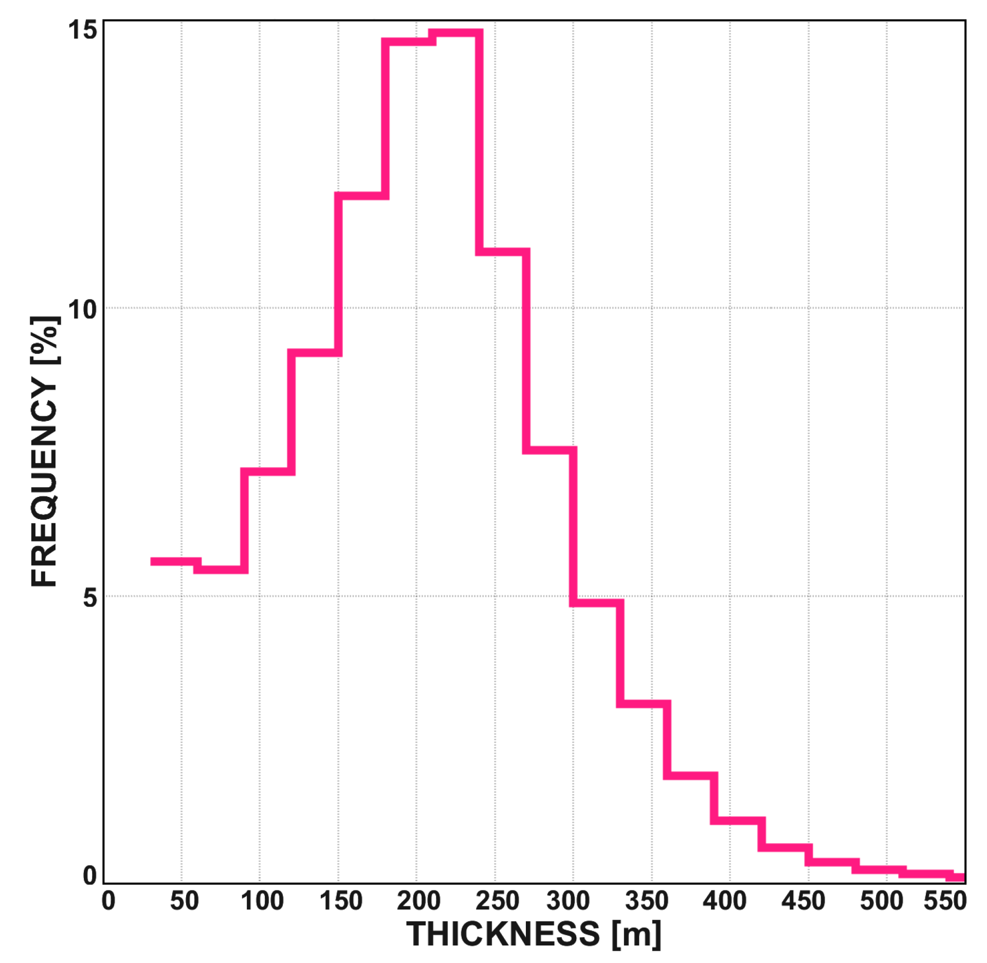
3.1. Cloud-Top SLW Vertical Thickness

Figure 1 exhibits the PDF of the “liquid-top” layer vertical thickness for the entire period of the NSA dataset and for all observed instances. The mean and standard deviation of the distribution are 188.7 and 72.4 m. Note that the 0.5 km criterion mentioned previously for the “liquid-top” vertical thickness is based on the observation that those layers rarely exceed 350–400 m.

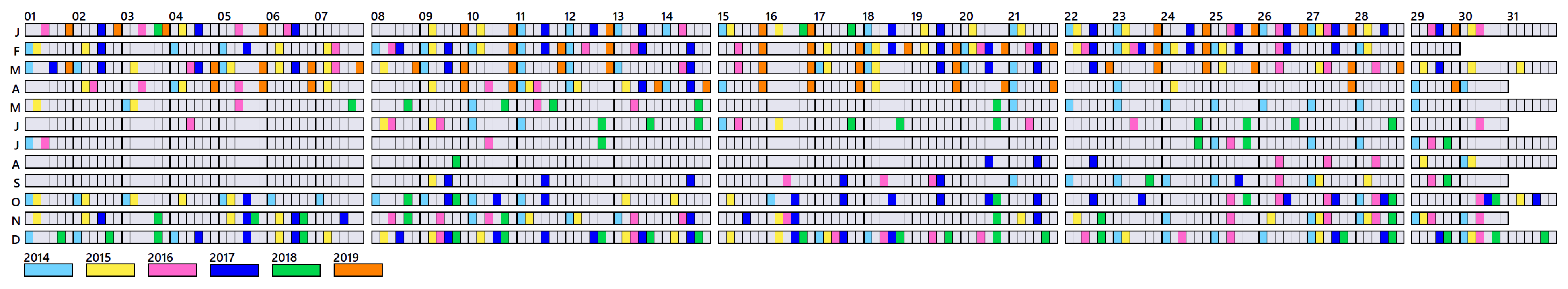
3.2. SLW Occurrence Frequency

Table 2 presents the total duration of both “liquid-top” and “liquid-embedded” instances, as classified by the radar–lidar synergy. Due to lidar attenuation, the occurrence values charted in columns 2 and 3 of Table 2 are certainly underestimated because a fraction of “liquid-top” or “liquid-embedded” duration may not be verifiable given the HSRL incidental extinction. Despite that, Table 2 shows that—on average—for the full-year periods (2014–2018) the annual “liquid-top” duration is 800–1000 h, while the “liquid-embedded” attains less values, at around 400 hrs. The presence of SLW in ice layers ( Z 20 dBZ) with minimum thickness of 1 km has been investigated. On average, 3000 hrs/year of such hydrometeor observations are observed at the NSA during the 2014–2018 period, and therefore “liquid-top” SLW occupies ∼25% of the total ice layer duration while “liquid-embedded” ∼10%.

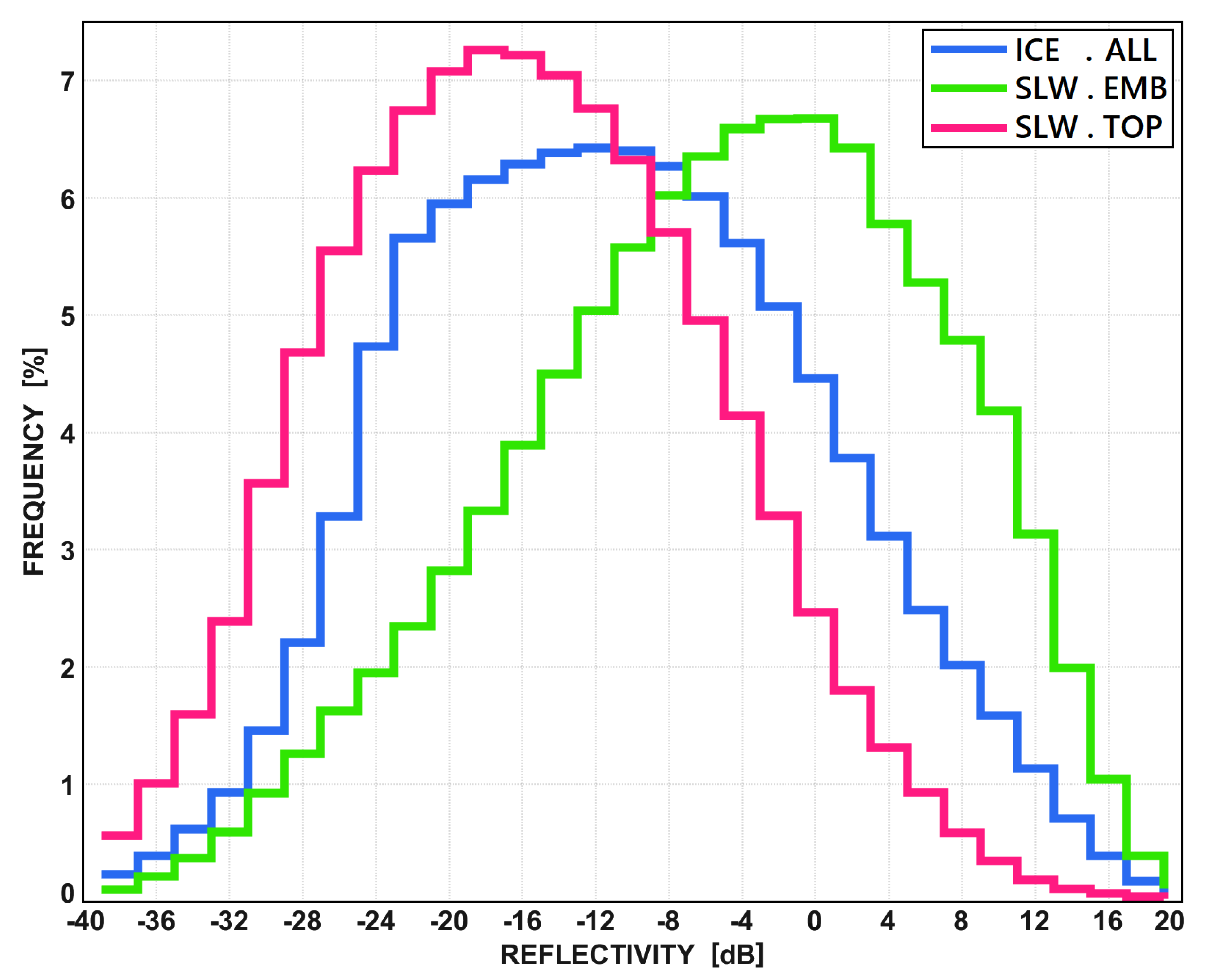
3.3. Reflectivity-Based PDFs per Hydrometeor Phase

Figure 2 shows the 35 GHz reflectivity distribution per cloud class for the entirety of the used dataset. One point of interest is that “liquid-embedded” generally appears within elevated reflectivities compared to the “liquid-top” class. The per-phase distribution most probable values (of the most frequently occurring Z-bins) is found for “liquid-top” in Z 18 dBZ whereas for “liquid-embedded” in Z 0 dBZ. For the “ice-all” cloud class, the most probable value of the corresponding curve is met at around 18 dBZ. An additional remark is that “liquid-top” is found typically in sub-zero reflectivities, as opposed to “liquid-embedded” that reaches as high as + 16 dBZ due to its co-existence with contiguous, high reflectivity ice.

4. Basis for Selection of the Radar-Based Variables
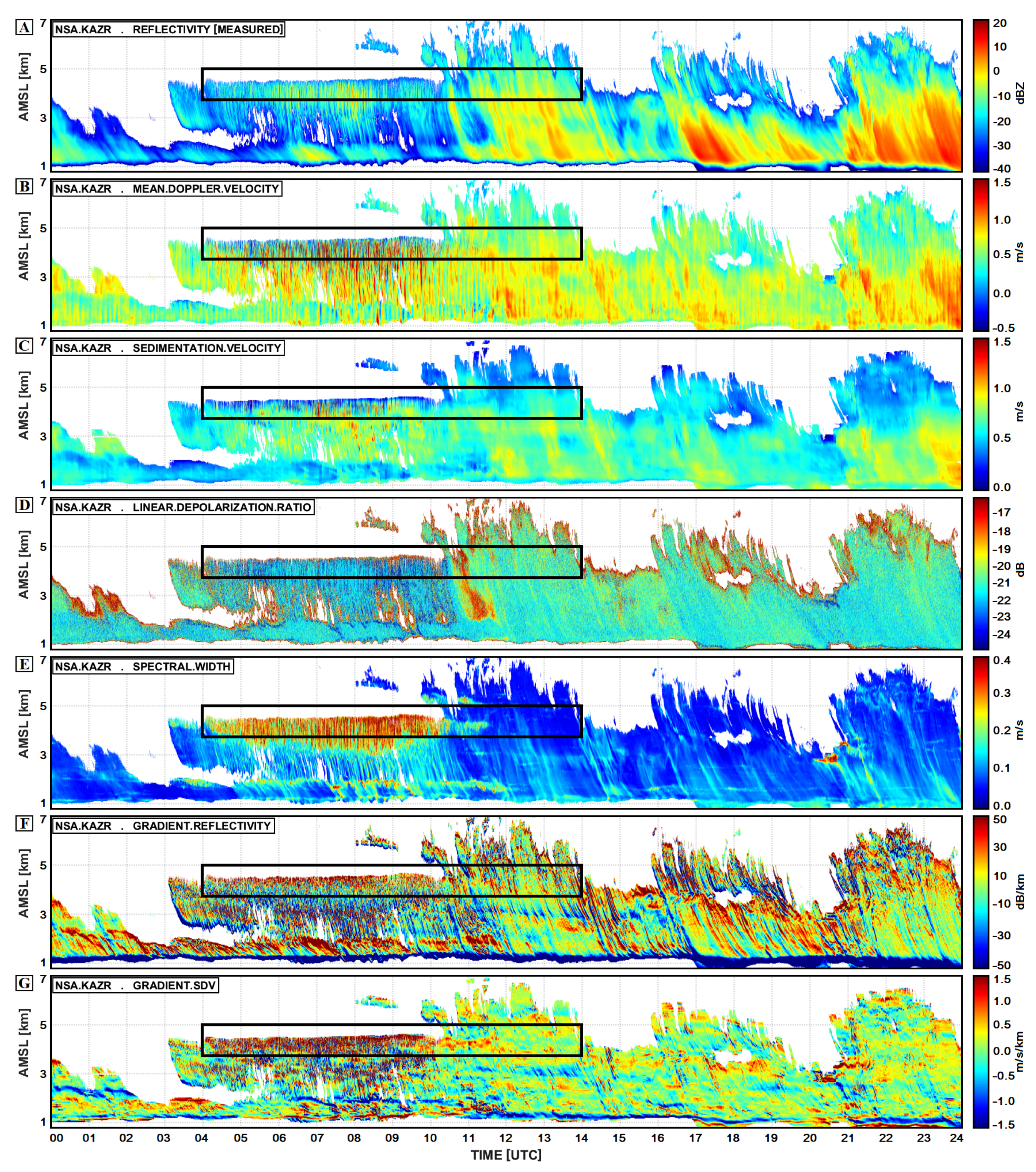
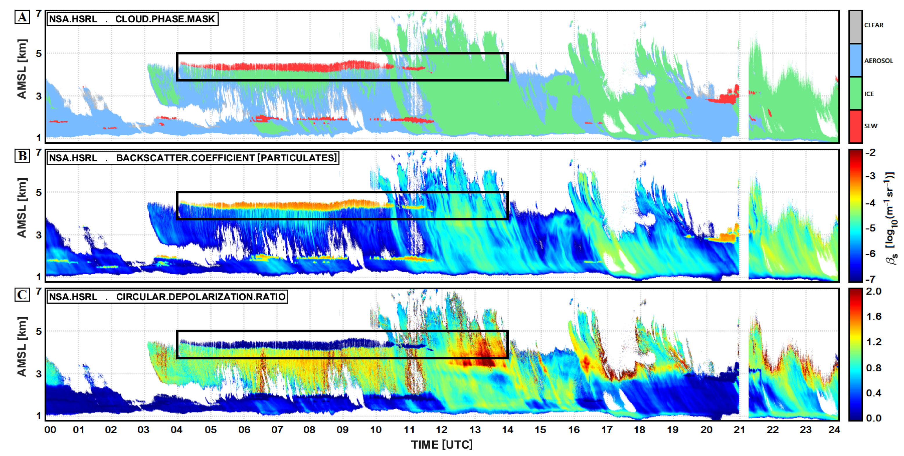
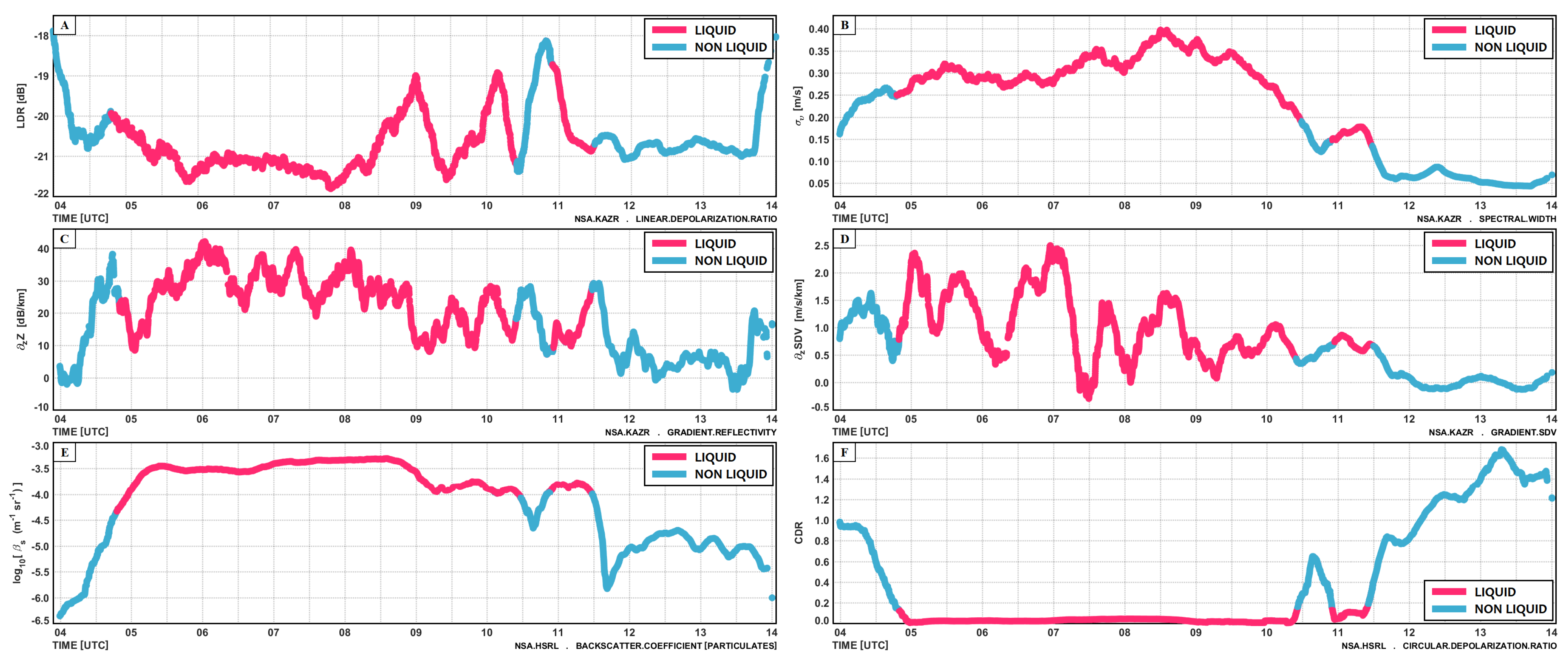
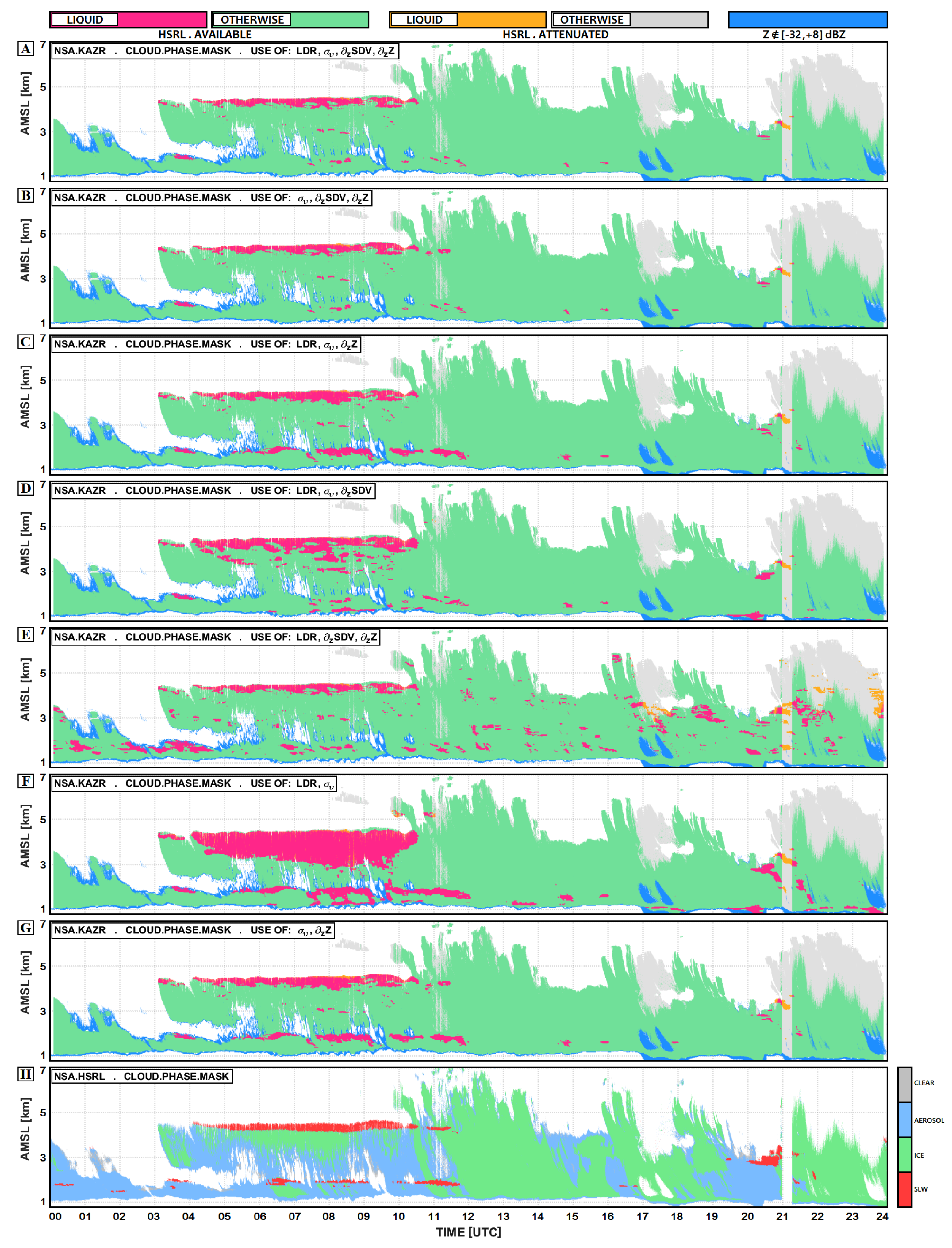
We have investigated different ice/liquid separation thresholds based on a variety of combination of the KaZR fields L D R , σ v , and vertical gradients of reflectivity z Z (dB km 1 ) and sedimentation velocity z S D V (m s 1 km 1 ). Non-radar fields are used for filtering and assessment. Namely, the HSRL β s and C D R are the main drivers of the lidar cloud phase mask, while ambient temperatures (T d r y ) exclude above-melting-point atmospheric regimes.
The fact that the NSA KaZR.MD is a dual-polarization receiver radar allows for the evaluation of radar-based L D R s at its operating frequency of 35 GHz. This variable is analyzed to ascertain whether the depolarization caused by discrepant ice/liquid geometric features and measured from profiling, mm-wavelength cloud radars is a viable option to be used in a radar-based phase partitioning, when full L D R spectra are not available (as opposed to the [31] findings). Regarding the motion variability, given the 5.5-year climatological examination of the NSA dataset, cold clouds exhibit a spectral width clustering around 0.10 m s 1 and rarely exceed 0.25 m s 1 . Conversely, within condensation zones atop clouds the spectral width is elevated to about 0.30 m s 1 . This is likely attributed to an enhancement in turbulence in the layer where supercooled liquid is present [30]. SLW drops have negligible fall velocity with near-zero differential fall velocities. Thus, the presence of enhance spectrum width (turbulence) is an indirect way of detecting the presence of the SLW. The vertical gradients mainly seek to differentiate sedimenting ice (previously deposited) whose growth rate may or may not be influenced by the presence of SLW; this is based on the assertion that the microphysical processes that condition the downwelling evolution of backscattering and sedimentation (in terms of a PSD size-broadening) may pinpoint the existence of SLW or otherwise. Of central interest remains the distinction in “liquid-top” and “liquid-embedded” because in the presence or absence of vapor competition with simultaneously growing ice (via Bergeron-Findeisen (see, e.g., in [51])), condensing liquid water is likely to attain diverse z Z and z S D V values.

4.1. Case Study

The portrayed case highlights a scene on 24 January with some characteristic behaviors. Figure 3A displays the reflectivity time-height pattern, panel (B) the mean Doppler velocity, panel (C) the sedimentation velocity, retrieved using the [49] method, panel (D) radar-based L D R , panel (E) spectral width, with panels (F,G) illustrating respectively the reflectivity and sedimentation velocity vertical gradients; Figure 4A shows the HSRL cloud phase mask that follows from the β s and C D R fields exhibited in Figure 4B,C. The bold black frame points to a regime of SLW presence, as demarcated by the lidar cloud mask.
At the smallest reflectivities ( Z < 30 dBZ), sampling volumes backscatter minimally, which suggests presence of distributed scatterers that are small-sized and/or sparse. At progressively greater reflectivities ( 30 up to + 20 dBZ) encountered at lower altitudes and usually higher temperatures, the ice-PSDs tends to size-broaden [52]. Qualitatively, mean ice hydrometeor size growth can be viewed by z Z (being positive or negative) as the reflectivity field is related to the hydrometeor volumetric growth. Mean Doppler velocities (Figure 3B) are signed quantities; by convention, positive-valued MDVs correspond to downwelling hydrometeor motions and negative-valued otherwise. Conversely, the M D V -derived S D V s (Figure 3C) are non-negative so that near-zero-valued S D V s point to a near-suspension of hydrometeors aloft, which is seen in non-precipitating, stratiform conditions. In principle, M D V equals the S D V plus a perturbation attributed to the vertical wind component (w) of the background flow. Thus, in dynamically quiescent conditions like the one illustrated here, it mostly is | M D V | S D V , with | w | 0.3 m s 1 . After 1100 UTC, L D R values cluster in the region of L D R 21 dB (Figure 3D) while the reflectivity elevates. During this frame the lidar mask (Figure 4A) registers ice-only cloud domains. During 0400–1100 UTC at about 4.5 km the lidar mask demarcates “liquid-top” presence of Z < 15 dBZ and L D R < 21 dB. If those volumes consist of spherically shaped liquid water droplets, smaller L D R s indicate hydrometeors that depolarize less than asymmetrically shaped frozen particulates. The Figure 1 PDF for cloud top SLW also suggests that this class is unlikely to be met for Z > 0 dBZ, which aligns with the recorded reflectivities seen in Figure 3A. Scenes of σ v [ 0.1 , 0.2 ] m s 1 point to dynamically more quiescent conditions, of less radial velocity variability. After 1100 UTC at all altitudes, it is σ v < 0.15 m s 1 (Figure 3E); these volumes correspond to ice-only domains. In the presence of condensing liquid water before 1100 UTC, either aloft (4.5 km) or below (2.0 km), the spectral width elevates, which is likely attributed to a rise in turbulence due to latent heat release assuming that other causalities that may increase σ v are less relevant. The radar-based panels of the vertical gradients for Z and S D V (Figure 3F,G) display fields that—by convention—are positive with decreasing altitude if the original field intensifies. A clustering of greater positive values in both z Z and z S D V is seen during the cloud top condensation zone (delineated by the black frame in each panel), than otherwise. Thereby, irrespective of the fact that ice backscatters much more than liquid droplets, what is examined via z Z is the downwelling evolution in growth of the related volumes; during the cloud top SLW formation (at 4.5 km) both gradients highlight such volumes of a sharp downwards increase in both Z and S D V within narrow vertical layers. Other regions of higher positive z Z do exist, yet the spectral widths therein are less than 0.1 m s 1 ; those volumes are not registered as liquid by the lidar.
The time series of Figure 5 showcases in further detail the evolution of the radar-based fields L D R , σ v , z Z , z S D V and the lidar-based β s and C D R at the fixed altitude 4.29 km, during 0353-1403 UTC. The time series correspond to the black-colored frame of Figure 3; according to the lidar mask (Figure 4A) cloud-top SLW formation is seen during 0500–1000 UTC, which is followed by ice after that time. While the L D R (panel (A)) does not show significant differentiations (within a margin of ± 0.5 dB) between the period with or without liquid (prior to or after 1000 UTC), the spectral width (panel (B)) shows a distinct transition at around 1000 UTC from high ( σ v = 0.3 m s 1 ) to low values (<0.1 m s 1 ). The Z and S D V vertical gradients (panels (C), (D)) present positive values during the “liquid-top” interval (0500–1000 UTC), while both fields subside to smaller values with the onset of ice after 1030 UTC. During the window identified as “liquid-top” by the lidar, z Z [ 10 , 40 ] dB km 1 , z S D V [ 0.0 , 2.5 ] m s 1 km 1 . On the other hand, after 1030 UTC, the time series shows z Z 15 dB km 1 and z S D V 0 m s 1 km 1 . Panels (E,F) portray the HSRL fields β s and C D R ; the HSRL thresholds of the liquid phase (Appendix A) are l o g 10 ( β s ) > l o g 10 ( 3 × 10 5 ) = 4.52 C D R < 0.1 , so that elevated values of σ v , z Z , and z S D V are seen to better correlate with the occurrence of the liquid phase. Given the radar-based L D R narrow dynamic range (centered at 21 dB), this variable seems less effective in identifying presence of SLW.

5. Methodology

The subsequent statistical analysis utilizes the three cloud-classes, as defined previously: (i) “ice-all”, (ii) “liquid-top”, and (iii) “liquid-embedded”. “Liquid-top” corresponds to SLW that appears within the first 0.5 km layer from cloud-top downwards, “liquid-embedded” to SLW encountered deeper within, and “ice-all” to the entirety of all ice pixels. The analysis proceeds with the formulation of combined datasets for each cloud class and each radar-based observable. The combined datasets are then segregated according to their reflectivities in 2-dB bins in [ 40 , + 20 ] dBZ. Climatological PDFs are produced for all radar-based variables of the three cloud classes within each Z-bin; the PDFs will be later used to derive criteria for the ice/liquid phase partitioning. The Z-binning is motivated by the fact that the reflectivity values roughly point to different stages of the ice growth process. For instance, close to cloud edges where Z < 20 dBZ, hydrometeor microphysical characteristics in size and shape may not be similar to cloud cores of Z > 5 dBZ, wherein a certain degree of aggregation has most likely occurred. It is not known beforehand how the volumetric growth may impact the resultant PDFs because relations across factors like radar reflectivity, ambient temperature (as that relates to collection efficiency), and particle state of motion are not easily verifiable. Therefore, the applied reflectivity segregation aims to offer an empirical description based entirely on observational evidence.

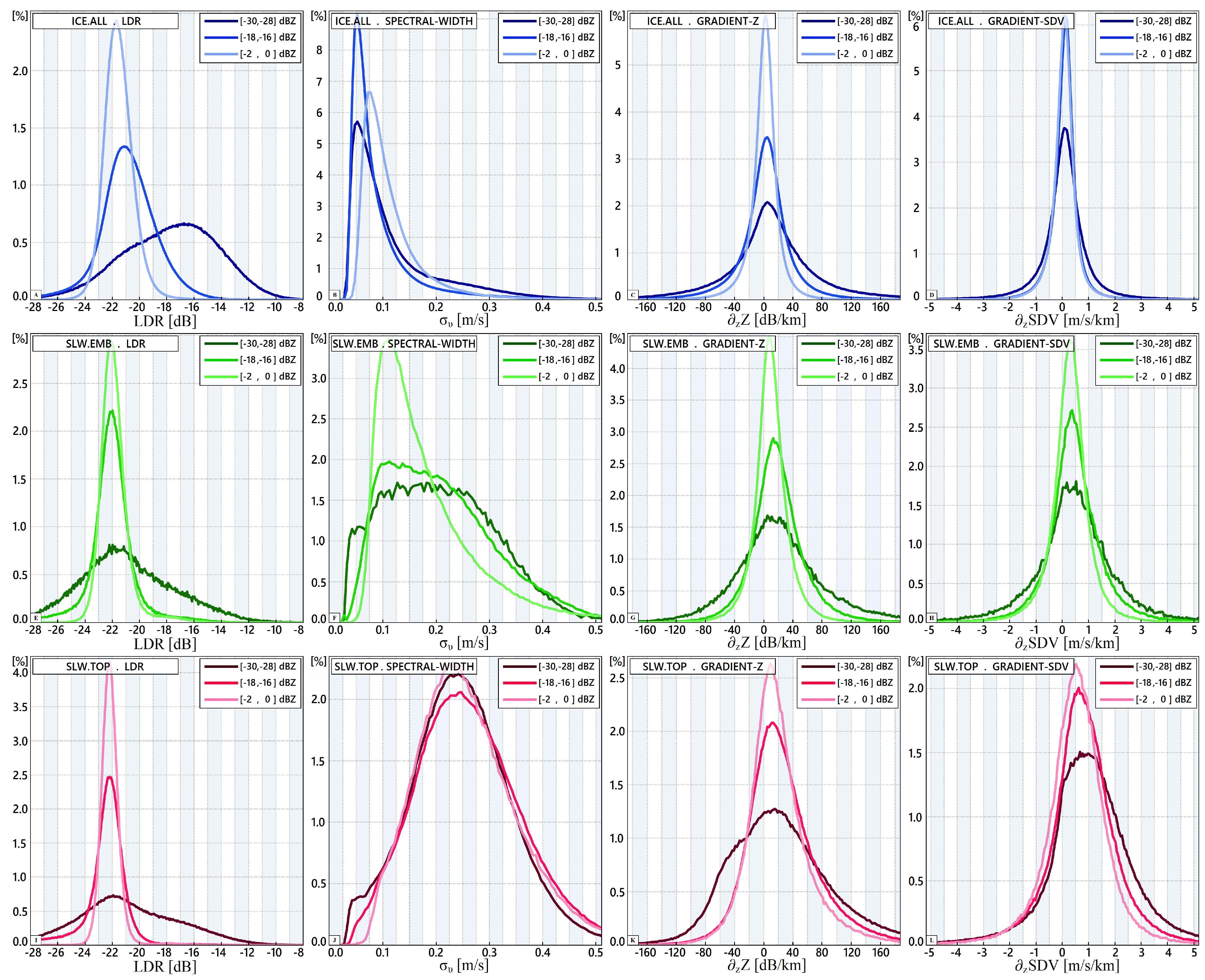
5.1. Climatological PDFs per Hydrometeor Phase

Figure 6 displays the climatological distributions of the examined NSA period. Each row pertains to a given cloud class and each column to each variable; rows 1, 2, and 3 are for “ice-all”, “liquid-embedded”, and “liquid-top”, respectively. Column 1 panels portray the L D R climatological distributions, column 2 the spectral width, with columns 3 and 4 the vertical gradients for Z and S D V . Only three reflectivity bin intervals are shown ( [ 30 , 28 ] , [ 18 , 16 ] , [ 2 , 0 ] dBZ) for clarity of presentation in Figure 6.
According to Equation (1), L D R depends on both VH and HH reflectivities. Reflectivity maintains an analogous relation with S N R so that at around −10 dB (in-cloud detection threshold assumed here) the correspondent reflectivities are no less than 40 dBZ (see Figure 3A). Sampling volumes of lower-end S N R s ( 0 dB) may result in more uncertain L D R evaluations. Still, this description pertains to a small data fraction of cloud edges as seen in Figure 3D, where the clustering in L D R 17 dB observed at the cloud tops after 1100 UTC is ostensibly greater than the L D R of all other in-cloud volumes. Climatologically, this is reflected in the L D R PDF panels (Figure 6A,E,I) for Z [ 30 , 28 ] dBZ, where (i) the right tails of the distributions reach values as high as 12 dB, and (ii) in the “ice-all” panel the distribution maximum is around 17 dB. Larger L D R s signify greater depolarization induced by the more asymmetrical particles, like pristine ice crystals, and therefore there is a physical basis for the climatological L D R PDF behavior at the smaller reflectivities. At progressively larger reflectivities, the L D R climatological clustering is seen near 22 dB, which is close to the KaZR antenna-induced L D R value. Smaller L D R s denote less depolarization attributed to more oblate scatterers, like water droplets and ice aggregates, met at greater reflectivities (see Figure 1). Here, in both Z-ranges [ 18 , 16 ] dBZ and [ 2 , 0 ] dBZ, the Figure 6 L D R PDF curves across all three cloud classes cluster similarly, suggesting (i) comparable depolarization in the broader Z-range of Z > 20 dBZ, (ii) positive asymmetries are only discerned in the “ice-all” L D R PDFs, and (iii) that the L D R narrow dynamic range undermines this variable’s applicability in the current context.
The panel (B) curves show that for “ice-all” the NSA spectral width climatological clustering is in σ v ( 0.00 , 0.15 ) m s 1 . The “liquid-embedded” σ v PDF curves (panel (F)) exhibit a behavior that is moderately reflectivity dependent; at progressively higher reflectivities both the mean values and dispersion decrease. The panel (J) σ v PDF curves for “liquid-top” showcase a reflectivity independence of the distribution parameters, as in “ice-all”. Yet, both panels (F), (J) exhibit a climatological clustering in σ v ( 0.1 , 0.4 ) m s 1 , which is discernibly elevated compared to “ice-all”.
Column 3, 4 panels ( z Z , z S D V ) illustrate that between “ice-all” and “liquid-embedded” the PDFs are morphologically quite similar, irrespective of reflectivity range. Conversely, the “liquid-top” distribution curves (Figure 6K,L) across all reflectivity ranges, exhibit positive asymmetries that skew their means towards elevated values for both gradients. Although positive skewness in both z Z and z S D V PDFs appears in the “liquid-embedded” class as well, it is more noticeable in the “liquid-top” distributions.

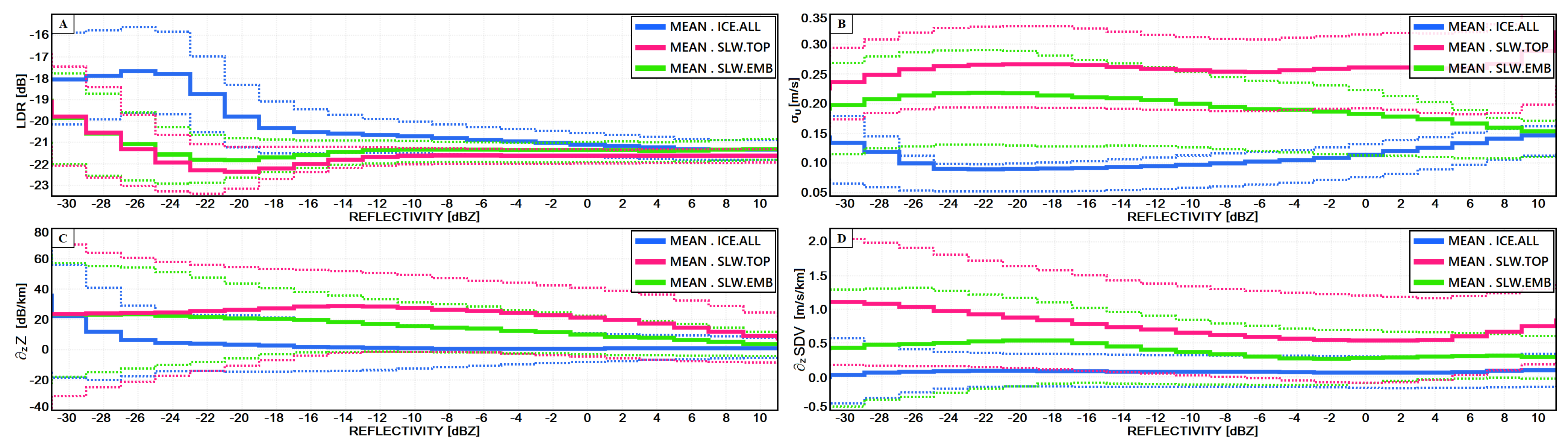
5.2. Phase Partition Thresholds

Figure 7 displays the reflectivity-segregated climatological PDF means of each radar variable and for each cloud class in Z [ 32 , + 12 ] dBZ. The 25% and 75% PDF percentiles of all three cloud classes across all four radar variables are also plotted in so further exemplifying the degree of overlap seen in those distributions. Figure 7A of the radar-based L D R indicates that the PDFs of the two liquid classes are highly similar (mean values and overall L D R 0.25 - L D R 0.75 dispersion almost indistinguishable). A point of interest is that up to Z 10 dBZ, a degree of separation between “ice-all” and “liquid-top” is maintained, as seen via the L D R 0.25 of the former and L D R 0.75 of the latter. Panel (B) for σ v exhibits good separation between “ice-all”/“liquid-embedded” irrespective of reflectivity. For this variable, the separation between “ice-all”/“liquid-top” is the most tangible, which, again, is observed via the ( σ v ) 0.25 of the cloud-top-liquid PDF against the ( σ v ) 0.75 for ice. Panel (C) of z Z displays greater mean values for “liquid-top” than “liquid-embedded”, of an overall behavior that, unlike in spectral width, is reflectivity dependent. The “liquid-top” z Z means commence from 25, maximize at 28, and gradually subside towards 10 dB km 1 at positive reflectivities. The “liquid-embedded” z Z means decrease monotonically, from 25 to 5 dB km 1 . This panel exhibits that for “ice-all” the mean value settles at z Z 0 dB km 1 . Reflectivity-gradient clustering in near-zero ranges points to cloudy domains wherein the downwelling volumetric growth is halted; phase transitions (i.e., deposition/sublimation or condensation/evaporation) are not likely to occur in those regimes because phase changes mark pronounced variations in reflectivity within narrow atmospheric layers. In the phase partition context, the “ice-all” habituation in z Z presents a characteristic behavior that may exclude the occurrence of water vapor condensation zones, as that is reflected via the climatological z Z PDF means for both liquid classes. Similar remarks are seen in panel (D), of the per-cloud-class z S D V climatological means. For “liquid-top”, these mean values do not fall below 0.5 m s 1 km 1 , whereas “liquid-embedded” cluster around 0.3 m s 1 km 1 . The “ice-all” class points to near-zero SDV vertical gradients, as is the case for the reflectivity ones.
The previous analysis already suggests that “liquid embedded” PDFs are less well separated than “liquid-top” from “ice-all” and that some variables (e.g., spectral width across all reflectivities and LDR for up to Z 10 dBZ) have more potential in distinguishing “ice-all” from “liquid-top” volumes. In the following, we will use the half-point of the climatological PDF means plotted in Figure 7 of the different cloud types as demarcation values between the ice/liquid phases. Such thresholds are used not on pointwise values of the examined radar observables but are applied to the mean values of the variables sampled in a local neighborhood. Such averaging should statistically move the sampled variables towards their climatological values. Therefore, differently from lidar state-of-the-art phase partitioning techniques that are applicable pixel by pixel on pointwise measurements, the radar technique proposed here exploits locally-sampled distribution parameters of radar observables. As a result, the technique should produce spatially coherent patches of clouds with the same phase.

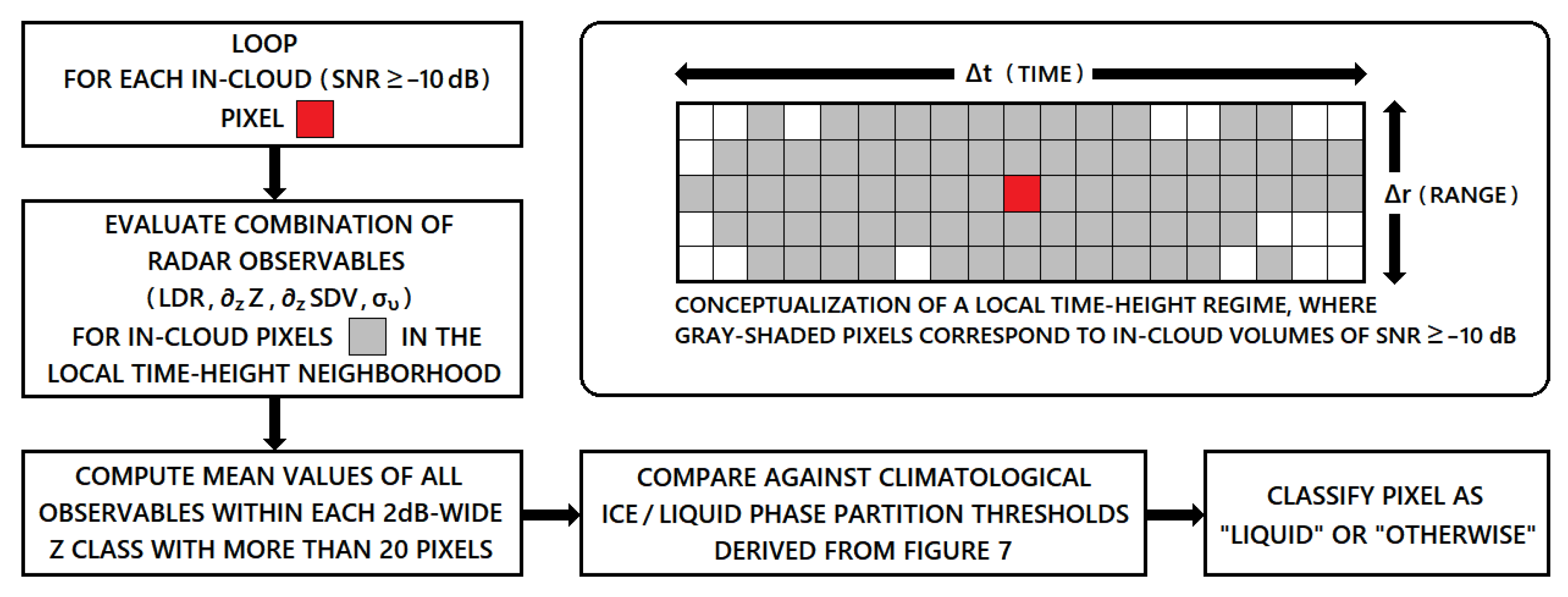
5.3. Radar-Based Cloud Mask Algorithm

The main steps of the algorithm are the following (see flowchart in Figure 8): (i) For an any given time-height domain (e.g., of a full day) the combined filtering of Z [ 32 , + 8 ] dBZ ∧ S N R 10 dB ∧ T d r y 0 ° C is applied across all four radar-based variables. (ii) For each pixel passing this criterion a local 10 min × 60 m sampling domain is considered, centered at it. (iii) For the application of the next steps at least half of the pixels in the local sampling domain must remain after the application of step (i). (iv) The pixels are binned according to 2 dB-wide reflectivity intervals in [ 32 , + 8 ] dBZ. When the pixel count across each 2-dB reflectivity bin is at least 20, the mean values of each radar-variable are computed. (v) The mean values of those locally-sampled distributions are compared against the phase partition thresholds. The phase of the pixel (centered at the local sampling domain) is attributed to “liquid” if more than half of the local means are less than the L D R climatological thresholds and greater than the climatological thresholds of the other radar-variables ( σ v , z Z , z S D V ). (vi) These steps are applied to all pixels thereby generating a binary radar-based cloud mask of two phase descriptors, “liquid” or “otherwise”.

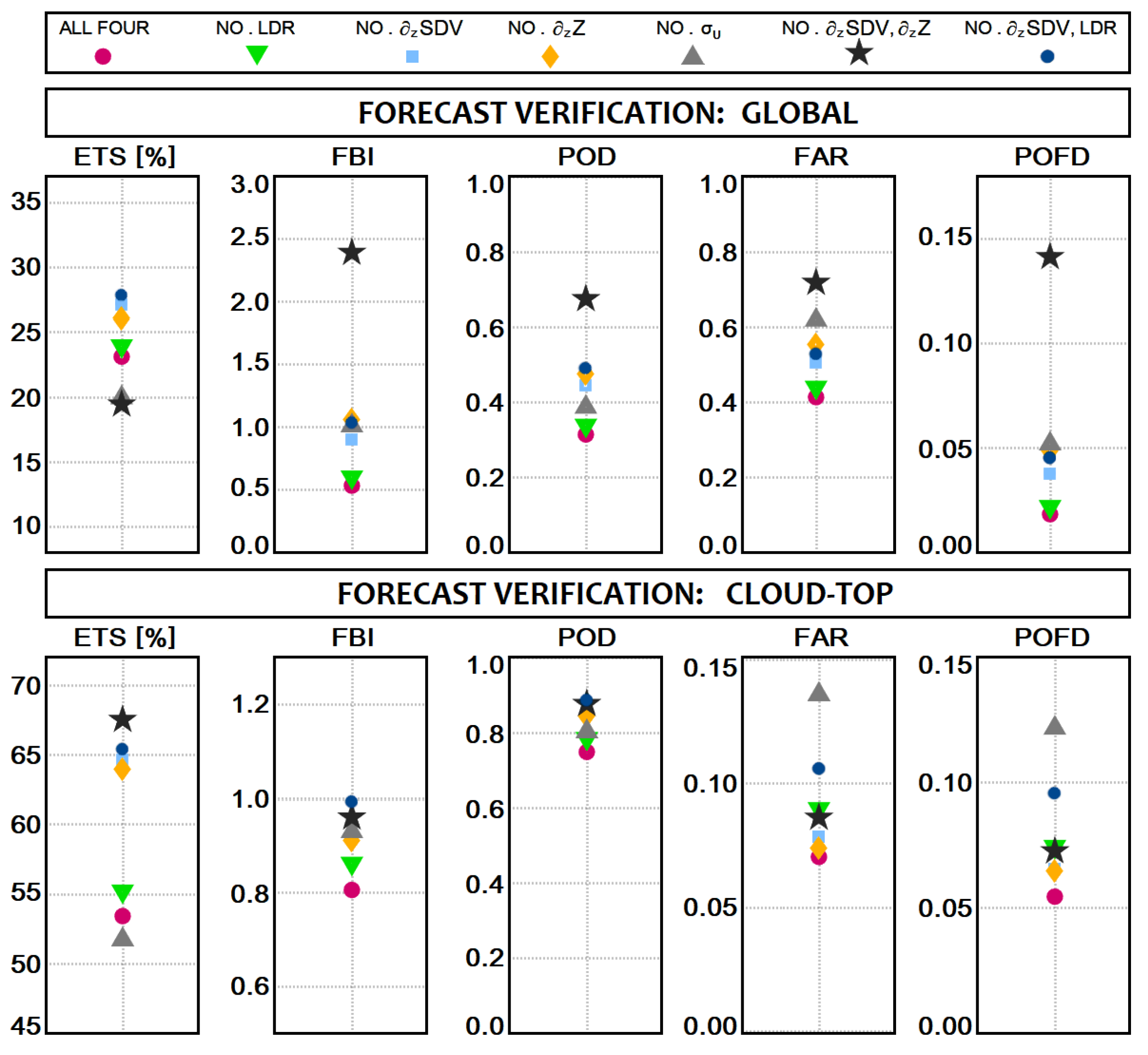
6. Forecast Verification Sensitivity Analysis

A sensitivity analysis of the effectiveness of the different combinations of the radar-based variables in the phase partitioning is carried out. To this end seven scenarios are considered for included variables in the technique’s execution: (i) all four, (ii) no L D R , (iii) no z S D V , (iv) no z Z , (v) no σ v , (vi) no z S D V and z Z (exclusion of both gradients), and (vii) no z S D V and L D R (no sedimentation/polarimetry).
Figure 9 portrays the application of the radar-based, cloud mask algorithm for the case previously explicated in Section 4.1. Seven combinations are considered (panels (A)–(G)) with the HSRL cloud phase mask (panel (H)) also shown for cross-comparison. Across panels (A)–(G) the same color scheme is applied: for the gamut of data-points wherein both radar and lidar are available the colors are magenta for the “radar-detected liquid” and green for “otherwise” (non-liquid as seen by the radar). For the volumes of an attenuated HSRL, the coloring changes to orange for the “radar-detected liquid” and gray for “otherwise”. The blue-colored pixels correspond to Z [ 32 , + 8 ] dBZ, wherein the algorithm is not applied due to the absence of phase separation thresholds at the lower or higher -end reflectivity ranges.
Figure 9 provides a general impression of the algorithm’s performance for each variable combination. Panels (A) all-four, (B) no L D R , (C) no z S D V , and (G) no z S D V and L D R behave similarly in highlighting “liquid-top” volumes during 0300-1030 UTC, at around 4 km. The SLW occurrence at 2 km is more clearly displayed in panels (C), (G). Panel (D) demonstrates a radar-based, “liquid-top” detection of a somewhat greater thickness than it appears in panel (H), while panel (E) highlights numerous misclassifications of ice-to-liquid when the spectral width is not incorporated. The most striking pattern of SLW overestimation is clearly seen in panel (F), in which case neither vertical gradient is applied.

6.1. Aggregate Statistics

The previously described algorithm was applied in 494 validation dates of the 2014–2019 NSA dataset period. Each validation date is visualized in the Figure 10 chart, all of which correspond to sub-freezing ambient temperatures. Dates of (i) a 24 h clear-sky state, (ii) a continual lidar extinction at the lowest altitudes (due to incidental ground fogs or low-level liquid water), and (iii) all bright-band signatures have been excluded.
The radar cloud mask is assessed via the lidar one, assumed as the truth. Two separate sets of filters are applied per sensor: for the radar those include Z [ 32 , + 8 ] dBZ ∧ S N R 10 dB ∧ T d r y 0   ° C (this defines the radar observation space, S R ), while for the lidar “non-attenuated” ∧ T d r y 0   ° C (this defines the lidar observation space, S L ). Therefore, the forecast verification can only occur for those volumes that are simultaneously observed by both sensors, i.e., S V S R S L ( S V ; validation space). Both cloud masks are binary; non-filtered pixels in the radar mask correspond to “liquid” or “non-liquid”, while in the lidar to “clear”, “aerosol”, “ice”, or “liquid” (Appendix A).
The forecast verification is quantified in terms of five statistical metrics [53]. These are the (i) Frequency Bias Index (FBI), (ii) Probability of Detection (POD), (iii) False Alarm Ratio (FAR), (iv) Probability of False Detection (POFD), and (v) Equitable Threat Score (ETS). These indices are evaluated from the four distinct populations of the contingencies (i) “hit” (radar, lidar)=(liquid, liquid), (ii) “false alarm” (radar, lidar)=(liquid, non-liquid), (iii) “miss” (radar, lidar)=(non-liquid, liquid), and (iv) “non-event” (radar, lidar)=(non-liquid, non-liquid), with the sum of all equal to the sample space size ( S V ).
In the contingency in Table 3, uppercase letters A, B, C, and D are assigned respectively to hit, false alarm, miss, and non-event. The five metrics are defined (i) FBI = ( A + B ) / ( A + C ) , (ii) POD = A / ( A + C ) , (iii) FAR = B / ( A + B ) , (iv) POFD = B / ( B + D ) , (v) ETS = ( A A r / A + B + C A r ) , where A r = ( A + B ) ( A + C ) / ( A + B + C + D ) (random hits population). The Frequency Bias Index (FBI 0 ) measures the degree of over-forecasting (>1) or under-forecasting (<1). POD [ 0 , 1 ] is the ratio of hits to the total lidar-detected “liquid” pixels. FAR [ 0 , 1 ] is the ratio of false alarms to the total radar-detected “liquid” pixels. POFD [ 0 , 1 ] is the ratio of false alarms to the total number of “non-liquid” pixels as observed by the lidar. Lastly, ETS [ 33 % , + 100 % ] is a metric that evaluates the overall skill level of the forecast. Perfect scores are achieved when FBI = POD = 1, FAR = POFD = 0, ETS = 100%. The forecast verification is implemented across two scenarios designated (i) “global”, for the entirety of the validation space S V and (ii) “cloud-top” for the pixel-fraction of S V that corresponds to the singular-highest radar and lidar -detected cloud tops that are simultaneously observed by both sensors, irrespective of phase.
Figure 11 panels visualize the aggregate statistics of all 494 validation dates separately for the global and the cloud-top forecast verification scenarios. In the upper row, panels appear the respective verification metrics of ETS, FBI, POD, FAR, and POFD for the global case, while in the lower row the corresponding ones for the cloud-top.
Figure 11 showcases ETSs of the global verification between 20% and 30%, depending on the variable combination. An ice/liquid phase partition of those skill levels is rather poor and marks the radar’s difficulty in correctly pinpointing embedded-in-ice SLW by application of this technique. One remark regarding the global verification FBI, POD, FAR, and POFD is that for the variable combination of “all-four” the corresponding metrics are at their lowest values. For this case FBI ≅ 0.5, exhibiting the most distinct SLW under-forecast, which is in accordance with the equally low POD ≅ 0.3. The FAR ≅ 0.4, POFD ≅ 0.02 for this combination reveal low ice-to-liquid misclassifications, although the number of hits is also the least. At the opposite end, “no z S D V and z Z ” (no gradients) results in a marked liquid-overestimation (FBI > 2), with the rest of the Figure 11 upper-row panels of this combination exhibiting the most numerous ice-to-liquid misclassifications throughout. The no-gradients run results in the minimum ETS (global) and shows that this approach should not be applied if at least one of the vertical gradients is not included.
The cloud-top aggregate statistics (lower-row Figure 11 panels) are quite dissimilar compared to the global. The ETSs for these cases are around 50–70%, and are therefore noticeably better compared to the global verification. The cloud-top FBI panel highlights values from 0.8 to 1 of a balanced “liquid-top” SLW forecasting (neither over-forecasted nor under-forecasted). Similarly, the POD panel displays a clustering of values close to unity, while the FAR and POFD do not exceed 0.15, thereby attaining close to perfect scores.
Table 4 charts in detail the forecast verification metrics (ETS, FBI, POD, FAR, POFD) in Z [ 32 , + 8 ] dBZ, for both global and cloud-top verification scenarios and for all seven radar-variable combinations. The key points of this table are (i) when including all four radar-variables in the global validation, the POD, FAR, and POFD are the least. This stems from the smallest number of hits and false alarms. Conversely, the number of misses is the greatest, which is reflected in the smallest FBI denoting a SLW under-forecast. Thus, the most constrained liquid-detection approach compared to the other six is the one where all four variables are considered. The same can be said for the cloud-top verification. (ii) When not including both vertical gradients in the global verification, both hits and false alarms are the largest throughout, with the least misses. This results in the largest FBI, POD, FAR, and POFD. In the cloud-top verification the contingencies are mitigated with less false alarms and misses, resulting in comparable metrics, if not better, with all other variable combinations. (iii) The seventh variable combination (use of σ v and z Z ) shows a good balance in all metrics for both global and cloud-top SLW-detection verifications. (iv) The runs that incorporate L D R s demonstrate highly similar statistics across all related verifications.
The aggregate statistics imply that if the objective is solely the detection of the SLW at cloud-tops, any of the variable combinations (i) no z S D V , (ii) no z Z , (iii) no z S D V and z Z , or (iv) no z S D V and L D R can be used. As the climatological “liquid-top” SLW-layer thickness is about 200 m (Section 3.3), radar-based cloud phase masks tailored to cloud-tops-only can be approximated via a resolution-dependent, liquid-pixel assignment at those snapshots where cloud-top SLW is actually detected. The inclusion of the radar-based L D R does not appear critical; therefore, this variable may be dropped without significant impact to the phase partition skill levels. One additional point is that S D V s stem from retrievals (the applied one is based on [49]), and are therefore affected by uncertainties that tend to increase in highly turbulent and convective scenarios. Because of that, z S D V may be less robust than the other variables when applied in the cloud-top SLW detection. Collectively, the optimal setup of the radar-based, phase partition algorithm, as applied in Z [ 32 , + 8 ] dBZ, is assigned to the pair of radar variables σ v and z Z that with a minimum number of variables shows SLW detection skill levels that are on par, or better, compared to the other combinations.

7. Summary

This study presented the formulation and assessment of a radar-only, moment-based methodology for the ice/liquid phase partitioning in arctic, mixed-phase conditions. The examined radar observables included linear depolarization ratio, spectral width, and vertical gradients of reflectivity and sedimentation velocity. The analysis covered a 5.5-year period of ARM NSA climate research facility data (January 2014–May 2019) collected by the polarimetric, Ka band Doppler profiler, the collocated HSRL, and radio sounding deployments.
Three cloud classes were formulated: (i) “ice-all”, (ii) “liquid-embedded”, and (iii) “liquid-top”. The “liquid-top” class corresponds to SLW that condenses atop clouds, whereas “liquid-embedded” to the liquid-cloud class that condenses among co-existing ice that partially inhibits its subsequent growth. According to Bergeron-Findeisen, relative humidity with respect to ice is less than for liquid. Therefore, in mixed-phase conditions should nucleation events (condensation, deposition) strain the water vapor availability, ice will grow preferentially to the liquid. Nevertheless, cloud condensation nuclei (CCN) and ice nuclei (IN) aerosol concentrations are highly impactful in the hydrometeor formation process; in IN-pristine conditions, liquid droplets atop clouds may initially grow uninhibited even if ice saturation ratios far surpass 100%. The phase discrimination workaround leaned on the hypothesis that the per-phase habituation in depolarization, velocity variability, and downwelling volumetric growth is discrepant enough that allows for an ice/liquid partitioning based on the clustering of radar observables like L D R , σ v , z Z , and z S D V within confined cloud domains.
The analysis concluded that radar-based polarimetry is not as critical as the lidar-based polarimetry. This statement leans on the premise that full radar-based LDR spectra may not be known, in which case moment-based methods like the one presented here can be considered as alternatives. Otherwise, radar-based polarimetry can be decisive in phase partitioning, as discussed in [31,33,34]. Moreover, derived information from the examination of the vertical gradients, particularly of reflectivity, is significant as is of the spectral width. This is viewed from the Section 6.1 aggregate statistics that demonstrated the most comprehensive SLW-detection skill levels in both global and cloud-top validation scenarios by application of just σ v and z Z . Overall, Doppler profilers entail a non-negligible phase partitioning skill that is considerably augmented when applied to the demarcation of cloud-top supercooled layers.
The study describes a radar-based phase partition methodology that can be regarded as a modular component applicable not only in high-latitude, mixed-phase cloud masking per se, but also in the refinement of the vertical distribution of path integrated liquid water amounts that are obtainable via MWR-based LWP retrievals (see, e.g., in [41]). That is, when cloud phase masks that rely on depolarization lidars, like the HSRL, are not available yet millimeter-radar attenuation correction because atmospheric propagation is necessitated, the radar-based phase partitioning can provide an alternative solution even if limited to cloud-tops only. In the context of research-oriented, multi-wavelength, multi-sensor cloud monitoring deployments for the quantitative retrieval of mixed-phase and ice microphysical properties the technique explicated here is of interest because it also pertains to signal attenuation correction when operating frequencies greater than 40 GHz are utilized. Therefore, to any research group the focus of which lies in ice and mixed-phase cloud property retrievals based on multi-wavelength conducts, W to G band cloud radars inclusive, the radar-based cloud phase masking may be of consideration given its capacity to demarcate lower-troposheric SLW, which affects the signal at higher frequencies in view of resulting path integrated attenuation amounts.
Note that the outlined technique has been tailored to a profiling sensor (chirp mode of the NSA KaZR) with hardware-specific characteristics like waveform and sensitivity. Other radars, ground-based or even spaceborne, entailing diversified calibrations, native resolutions, sensitivity, or deployment methods (in relation to antenna motions) may significantly alter key variables such as the reflectivity field or the spectral width, and therefore caution is advised in the generalization of the procedure proposed in this study.

Author Contributions

P.K. (Petros Kalogeras) did the full analysis and drafted the paper; A.B. supervised the work and helped reviewing the draft; P.K. (Pavlos Kollias) reviewed the paper. All authors have read and agreed to the published version of the manuscript.

Funding

The work was funded by the by US Atmospheric System Research (grant no. DESC0017967), P.K. (Pavlos Kollias) was supported by the US Department of Energy (DOE) Atmospheric System Research Program under contract DE-SC0012704.

Institutional Review Board Statement

Not applicable.

Informed Consent Statement

Not applicable.

Conflicts of Interest

The authors declare no conflict of interest. The funders had no role in the design of the study; in the collection, analyses, or interpretation of data; in the writing of the manuscript; or in the decision to publish the results.

Appendix A. HSRL Hydrometeor Phase Mask

The HSRL hydrometeor classification occurs using the combined measurements of backscattering coefficient β s (m 1 sr 1 ) and circular depolarization ratio ( C D R ). Table A1 presents the combined criteria of both β s and C D R that produce on a per-pixel basis the HSRL cloud phase mask, which is a binary field with four descriptors, each one corresponding to the related atmospheric class as shown in Table A1.
Table A1. HSRL atmospheric classification criteria in terms of backscattering coefficient ( β s ) and circular depolarization ratio ( C D R ). Symbol ∧ represents the logical intersection. Based on [29].
β s (m 1 sr 1 ) C D R CLASS
< 1 × 10 7 > 0.00 CLEAR
> 1 × 10 7     < 1 × 10 6 > 0.00 AEROSOL
> 1 × 10 6     < 3 × 10 5 < 0.25 AEROSOL
> 3 × 10 5 < 0.10 LIQUID
> 1 × 10 6     < 3 × 10 5 > 0.25 ICE
> 3 × 10 5 > 0.10 ICE

Appendix B. Vertical Gradients

The computational method for evaluating vertical gradients of any profiling radar field is in terms of the following three equations:
y i = 1 Δ h 4 5 ( y i + 1 y i 1 ) 1 5 ( y i + 2 y i 2 ) + 4 105 ( y i + 3 y i 3 ) 1 280 ( y i + 4 y i 4 ) + O ( Δ h 8 ) ,
y i = 1 Δ h 25 12 y i + 4 y i + 1 3 y i + 2 + 4 3 y i + 3 1 4 y i + 4 + O ( Δ h 4 ) ,
  y i = 1 Δ h 25 12 y i 4 y i 1 + 3 y i 2 4 3 y i 3 + 1 4 y i 4 + O ( Δ h 4 ) .
This numerical approach uses higher-order, first derivative, numerical formulas of one-way (forward, backward) or centered schemes. Equation (A1) pertains to the order-8 centered schemes (derived via superimpositions of forward and backward Taylor series expansions), while Equations (A2) and (A3) to the order-4 one-way schemes (derived from the differentiation of the Newton–Gregory polynomials). Index i denotes the spatial position in the data-grid (range bin), Δ h is the spatial step (gate spacing of 30 m), y represents the radar field, and y its first derivative. Vertical gradients are assumed positive with decreasing altitude if the original field intensifies and negative if it lessens. At cloud edges (at the four outermost pixels), the used formulas are the one-way; at cloud-bottoms via Equation (A2) (forward) that applies information only from the domain of the higher range bins, while at cloud-tops via Equation (A3) (backward). As the centered measurements are twice as accurate as the one-way, all other in-cloud gradients are evaluated pixel-wise by Equation (A1) that requires two-sided information from the nearest four neighboring data-points.

References

  1. Cober, S.G.; Isaac, G.A.; Korolev, A.V.; Strapp, J.W. Assessing Cloud-Phase Conditions. J. Appl. Meteorol. 2001, 40, 1967–1983. [Google Scholar] [CrossRef]
  2. Platt, C.M.R. Lidar Observation of a Mixed-Phase Altostratus Cloud. J. Appl. Meteorol. 1977, 16, 339–345. [Google Scholar] [CrossRef] [Green Version]
  3. Heymsfield, A.J.; Milosevich, L.M.; Slingo, A.; Sassen, K.; Starr, D.O. An observational and theoretical study of highly supercooled altocumulus. J. Atmos. Sci. 1991, 48, 923–945. [Google Scholar] [CrossRef] [Green Version]
  4. Gayet, J.F.; Asano, S.; Yamazaki, A.; Uchiyama, A.; Sinyuk, A.; Jourdan, O.; Auriol, F. Two case studies of winter continental-type water and mixed-phase stratocumuli over the sea 1. Microphysical and optical properties. J. Geophys. Res. Atmos.s 2002, 107, AAC 11–1–AAC 11–15. [Google Scholar] [CrossRef]
  5. Lubin, D. Thermodynamic phase of maritime Antarctic clouds from FTIR and supplementary radiometric data. J. Geophys. Res. Atmos. 2004, 109. [Google Scholar] [CrossRef] [Green Version]
  6. Hogan, R.J.; Behera, M.D.; O’Connor, E.J.; Illingworth, A.J. Estimate of the global distribution of stratiform supercooled liquid water clouds using the LITE lidar. Geophys. Res. Lett. 2004, 31. [Google Scholar] [CrossRef] [Green Version]
  7. Lubin, D.; Chen, B.; Bromwich, D.H.; Somerville, R.C.J.; Lee, W.H.; Hines, K.M. The Impact of Antarctic Cloud Radiative Properties on a GCM Climate Simulation. J. Clim. 1998, 11, 447–462. [Google Scholar] [CrossRef] [Green Version]
  8. Trenberth, K.E.; Fasullo, J.T.; Kiehl, J. Earth’s Global Energy Budget. Bull. Am. Meteorol. Soc. 2009, 90, 311–324. [Google Scholar] [CrossRef]
  9. Li, Z.X.; Le Treut, H. Cloud-radiation feedbacks in a general circulation model and their dependence on cloud modelling assumptions. Clim. Dyn. 1992, 7, 133–139, Provided by the SAO/NASA Astrophysics Data System. [Google Scholar] [CrossRef]
  10. Stephens, G.L.; Tsay, S.C.; Stackhouse, P.W.; Flatau, P.J. The Relevance of the Microphysical and Radiative Properties of Cirrus Clouds to Climate and Climatic Feedback. J. Atmos. Sci. 1990, 47, 1742–1754. [Google Scholar] [CrossRef]
  11. McCoy, D.T.; Hartmann, D.L.; Zelinka, M.D.; Ceppi, P.; Grosvenor, D.P. Mixed-phase cloud physics and Southern Ocean cloud feedback in climate models. J. Geophys. Res. Atmos. 2015, 120, 9539–9554. [Google Scholar] [CrossRef]
  12. Lawson, R.P.; Baker, B.A.; Schmitt, C.G.; Jensen, T.L. An overview of microphysical properties of Arctic clouds observed in May and July 1998 during FIRE ACE. J. Geophys. Res. Atmos. 2001, 106, 14989–15014. [Google Scholar] [CrossRef] [Green Version]
  13. Bennartz, R.; Shupe, M.D.; Turner, D.D.; Walden, V.P.; Steffen, K.; Cox, C.J.; Kulie, M.S.; Miller, N.B.; Pettersen, C. July 2012 Greenland melt extent enhanced by low-level liquid clouds. Nature 2013, 496, 83–86. [Google Scholar] [CrossRef]
  14. Kikuchi, M.; Okamoto, H.; Sato, K.; Suzuki, K.; Cesana, G.; Hagihara, Y.; Takahashi, N.; Hayasaka, T.; Oki, R. Development of Algorithm for Discriminating Hydrometeor Particle Types With a Synergistic Use of CloudSat and CALIPSO. J. Geophys. Res. Atmos. 2017, 122, 11022–11044. [Google Scholar] [CrossRef]
  15. Sun, Z.; Shine, K.P. Studies of the radiative properties of ice and mixed-phase clouds. Q. J. R. Meteorol. Soc. 1994, 120, 111–137. [Google Scholar] [CrossRef]
  16. Gregory, D.; Morris, D. The sensitivity of climate simulation to the specification of mixed phase clouds. Clim. Dyn. 1996, 12, 641–651. [Google Scholar] [CrossRef]
  17. Shupe, M.D.; Intrieri, J.M. Cloud Radiative Forcing of the Arctic Surface: The Influence of Cloud Properties, Surface Albedo, and Solar Zenith Angle. J. Clim. 2004, 17, 616–628. [Google Scholar] [CrossRef]
  18. Field, P.R. Aircraft Observations of Ice Crystal Evolution in an Altostratus Cloud. J. Atmos. Sci. 1999, 56, 1925–1941. [Google Scholar] [CrossRef]
  19. Wang, Z.; Sassen, K.; Whiteman, D.N.; Demoz, B.B. Studying Altocumulus with Ice Virga Using Ground-Based Active and Passive Remote Sensors. J. Appl. Meteorol. 2004, 43, 449–460. [Google Scholar] [CrossRef]
  20. Shupe, M.D.; Daniel, J.S.; de Boer, G.; Eloranta, E.W.; Kollias, P.; Long, C.N.; Luke, E.P.; Turner, D.D.; Verlinde, J. A Focus On Mixed-Phase Clouds. Bull. Am. Meteorol. Soc. 2008, 89, 1549–1562. [Google Scholar] [CrossRef] [Green Version]
  21. Hu, Y.; Rodier, S.; Xu, K.M.; Sun, W.; Huang, J.; Lin, B.; Zhai, P.; Josset, D. Occurrence, liquid water content, and fraction of supercooled water clouds from combined CALIOP/IIR/MODIS measurements. J. Geophys. Res. Atmos. 2010, 115. [Google Scholar] [CrossRef]
  22. Battaglia, A.; Delanoë, J. Synergies and complementarities of CloudSat-CALIPSO snow observations. J. Geophys. Res. Atmos. 2013, 118, 721–731. [Google Scholar] [CrossRef] [Green Version]
  23. Sassen, K. Deep Orographic Cloud Structure and Composition Derived from Comprehensive Remote Sensing Measurements. J. Clim. Appl. Meteorol. 1984, 23, 568–583. [Google Scholar] [CrossRef] [Green Version]
  24. Sassen, K. The Polarization Lidar Technique for Cloud Research: A Review and Current Assessment. Bull. Am. Meteorol. Soc. 1991, 72, 1848–1866. [Google Scholar] [CrossRef]
  25. Intrieri, J.M.; Shupe, M.D.; Uttal, T.; McCarty, B.J. An annual cycle of Arctic cloud characteristics observed by radar and lidar at SHEBA. J. Geophys. Res. Ocean. 2002, 107, SHE 5–1–SHE 5–15. [Google Scholar] [CrossRef]
  26. Miller, S.W.; Emery, W.J. An Automated Neural Network Cloud Classifier for Use over Land and Ocean Surfaces. J. Appl. Meteorol. 1997, 36, 1346–1362. [Google Scholar] [CrossRef]
  27. Baum, B.A.; Tovinkere, V.; Titlow, J.; Welch, R.M. Automated Cloud Classification of Global AVHRR Data Using a Fuzzy Logic Approach. J. Appl. Meteorol. 1997, 36, 1519–1540. [Google Scholar] [CrossRef] [Green Version]
  28. Wang, Z.; Sassen, K. Cloud Type and Macrophysical Property Retrieval Using Multiple Remote Sensors. J. Appl. Meteorol. 2001, 40, 1665–1682. [Google Scholar] [CrossRef]
  29. Shupe, M.D. A ground-based multisensor cloud phase classifier. Geophys. Res. Lett. 2007, 34. [Google Scholar] [CrossRef] [Green Version]
  30. Luke, E.P.; Kollias, P.; Shupe, M.D. Detection of supercooled liquid in mixed-phase clouds using radar Doppler spectra. J. Geophys. Res. Atmos. 2010, 115. [Google Scholar] [CrossRef] [Green Version]
  31. Luke, E.P.; Yang, F.; Kollias, P.; Vogelmann, A.M.; Maahn, M. New insights into ice multiplication using remote-sensing observations of slightly supercooled mixed-phase clouds in the Arctic. Proc. Natl. Acad. Sci. USA 2021, 118, e2021387118. [Google Scholar] [CrossRef] [PubMed]
  32. Silber, I.; Verlinde, J.; Wen, G.; Eloranta, E.W. Can Embedded Liquid Cloud Layer Volumes Be Classified in Polar Clouds Using a Single-Frequency Zenith-Pointing Radar? IEEE Geosci. Remote. Sens. Lett. 2019, 17, 222–226. [Google Scholar] [CrossRef]
  33. Kalesse, H.; de Boer, G.; Solomon, A.; Oue, M.; Ahlgrimm, M.; Zhang, D.; Shupe, M.D.; Luke, E.; Protat, A. Understanding Rapid Changes in Phase Partitioning between Cloud Liquid and Ice in Stratiform Mixed-Phase Clouds: An Arctic Case Study. Mon. Weather. Rev. 2016, 144, 4805–4826. [Google Scholar] [CrossRef]
  34. Oue, M.; Kollias, P.; Ryzhkov, A.; Luke, E.P. Toward Exploring the Synergy Between Cloud Radar Polarimetry and Doppler Spectral Analysis in Deep Cold Precipitating Systems in the Arctic. J. Geophys. Res. Atmos. 2018, 123, 2797–2815. [Google Scholar] [CrossRef]
  35. Kollias, P.; Bharadwaj, N.; Clothiaux, E.E.; Lamer, K.; Oue, M.; Hardin, J.; Isom, B.; Lindenmaier, I.; Matthews, A.; Luke, E.P.; et al. The ARM Radar Network: At the Leading-edge of Cloud and Precipitation Observations. BAMS 2020. [Google Scholar] [CrossRef] [Green Version]
  36. Verlinde, J.; Zak, B.D.; Shupe, M.D.; Ivey, M.D.; Stamnes, K. The ARM North Slope of Alaska (NSA) Sites. Meteorol. Monogr. 2016, 57, 8.1–8.13. [Google Scholar] [CrossRef]
  37. Widener, K.; Bharadwaj, N.; Johnson, K. Ka-Band ARM Zenith Radar (KAZR) Instrument Handbook; PNNL: Richland, WA, USA, 2012.
  38. Kollias, P.; Clothiaux, E.E.; Ackerman, T.P.; Albrecht, B.A.; Widener, K.B.; Moran, K.P.; Luke, E.P.; Johnson, K.L.; Bharadwaj, N.; Mead, J.B.; et al. Development and Applications of ARM Millimeter-Wavelength Cloud Radars. Meteorol. Monogr. 2016, 57, 17.1–17.19. [Google Scholar] [CrossRef]
  39. Eloranta, E.W. High Spectral Resolution Lidar. In High Spectral Resolution Lidar, in Lidar: Range-Resolved Optical Remote Sensing of the Atmosphere; Springer: New York, NY, USA, 2005; Chapter 5. [Google Scholar]
  40. Liebe, H.J. An updated model for millimeter wave propagation in moist air. Radio Sci. 1985, 20, 1069–1089. [Google Scholar] [CrossRef] [Green Version]
  41. Cadeddu, M.P.; Liljegren, J.C.; Turner, D.D. The Atmospheric radiation measurement (ARM) program network of microwave radiometers: Instrumentation, data, and retrievals. Atmos. Meas. Tech. 2013, 6, 2359–2372. [Google Scholar] [CrossRef] [Green Version]
  42. Lhermitte, R. Attenuation and Scattering of Millimeter Wavelength Radiation by Clouds and Precipitation. J. Atmos. Ocean. Technol. 1990, 7, 464–479. [Google Scholar] [CrossRef] [Green Version]
  43. Hogan, R.J.; Illingworth, A.J. The Potential of Spaceborne Dual-Wavelength Radar to Make Global Measurements of Cirrus Clouds. J. Atmos. Ocean. Technol. 1999, 16, 518–531. [Google Scholar] [CrossRef]
  44. Doviak, R.J.; Zrnicć, D.S. Doppler Radar and Weather Observations, 2nd ed.; Academic Press: San Diego, CA, USA, 1993; 562p. [Google Scholar]
  45. Görsdorf, U.; Lehmann, V.; Bauer-Pfundstein, M.; Peters, G.; Vavriv, D.; Vinogradov, V.; Volkov, V. A 35-GHz Polarimetric Doppler Radar for Long-Term Observations of Cloud Parameters—Description of System and Data Processing. J. Atmos. Ocean. Technol. 2015, 32, 675–690. [Google Scholar] [CrossRef]
  46. Di Girolamo, P.; Summa, D.; Cacciani, M.; Norton, E.G.; Peters, G.; Dufournet, Y. Lidar and radar measurements of the melting layer: Observations of dark and bright band phenomena. Atmos. Chem. Phys. 2012, 12, 4143–4157. [Google Scholar] [CrossRef] [Green Version]
  47. Myagkov, A.; Seifert, P.; Wandinger, U.; Bühl, J.; Engelmann, R. Relationship between temperature and apparent shape of pristine ice crystals derived from polarimetric cloud radar observations during the ACCEPT campaign. Atmos. Meas. Tech. 2016, 9, 3739–3754. [Google Scholar] [CrossRef] [Green Version]
  48. Bühl, J.; Seifert, P.; Myagkov, A.; Ansmann, A. Measuring ice- and liquid-water properties in mixed-phase cloud layers at the Leipzig Cloudnet station. Atmos. Chem. Phys. 2016, 16, 10609–10620. [Google Scholar] [CrossRef] [Green Version]
  49. Kalesse, H.; Kollias, P. Climatology of High Cloud Dynamics Using Profiling ARM Doppler Radar Observations. J. Clim. 2013, 26, 6340–6359. [Google Scholar] [CrossRef]
  50. Protat, A.; Williams, C.R. The Accuracy of Radar Estimates of Ice Terminal Fall Speed from Vertically Pointing Doppler Radar Measurements. J. Appl. Meteorol. Climatol. 2011, 50, 2120–2138. [Google Scholar] [CrossRef]
  51. Lamb, D.; Verlinde, J. Physics and Chemistry of Clouds, 1st ed.; Cambridge University Press: Cambridge, UK, 2011; 584p. [Google Scholar]
  52. Field, P.R.; Heymsfield, A.J.; Bansemer, A. Snow Size Distribution Parameterization for Midlatitude and Tropical Ice Clouds. J. Atmos. Sci. 2007, 64, 4346–4365. [Google Scholar] [CrossRef]
  53. Wilks, D. Forecast Verification. In Statistical Methods in the Atmospheric Sciences, 2nd ed.; Academic Press: Oxford, UK, 2006; Chapter 7. [Google Scholar]
Figure 1. Relative frequency diagram of the observed “liquid-top” layer vertical thickness for the NSA site (January 2014–May 2019).
Remotesensing 13 02891 g001
Figure 2. Relative frequency diagram as a function of the KaZR.MD reflectivity for the cloud classes “ice-all” (blue), “liquid-embedded” (green), and “liquid-top” (magenta), pertaining to the data-union of the examined NSA period (January 2014–May 2019). Samples are clustered in 2-dB reflectivity bins in [ 40 , + 20 ] dBZ.
Remotesensing 13 02891 g002
Figure 3. Time-height plots of the 24 January 2019 case for the KaZR.MD fields (A) measured reflectivity (Z), (B) observed mean Doppler velocity ( M D V ), (C) retrieved sedimentation velocity ( S D V ), (D) radar-based linear depolarization ratio ( L D R ), (E) spectral width ( σ v ), (F) reflectivity vertical gradient ( z Z ), and (G) sedimentation velocity vertical gradient ( z S D V ). The black-colored frame demarcates a cloud-top SLW region highlighted in detail in Figure 5.
Remotesensing 13 02891 g003
Figure 4. As in Figure 3 for the HSRL fields (A) binary cloud phase mask, (B) particulate’s backscattering coefficient ( β s ), and (C) circular depolarization ratio ( C D R ).
Remotesensing 13 02891 g004
Figure 5. Time series during 0353–1403 UTC, at the fixed altitude of 4.29 km (AMSL) of fields shown in Figure 3 and Figure 4: (A) radar-based linear depolarization ratio, (B) spectral width, (C) reflectivity vertical gradient, (D) S D V vertical gradient, (E) HSRL backscattering coefficient, (F) HSRL circular depolarization ratio.
Remotesensing 13 02891 g005
Figure 6. Relative frequency diagrams of the radar-based variables at three select reflectivity bins for the NSA dataset (January 2014–May 2019) corresponding to “ice-all” (blue), “liquid-embedded” (green), and “liquid-top” (magenta) cloud classes. Each row pertains to each cloud class. Column 1 panels (A,E,I) portray the PDFs for L D R , column 2 (B,F,J) spectral width ( σ v ), column 3 (C,G,K) reflectivity-gradient ( z Z ), and column 4 (D,H,L) S D V -gradient ( z S D V ). Each curve color corresponds to the reflectivity bin as indicated in the panel legends.
Remotesensing 13 02891 g006
Figure 7. Climatological PDF mean values of the cloud classes “ice-all” (solid blue), “liquid-embedded” (solid green), and “liquid-top” (solid magenta) as a function of the KaZR.MD reflectivity in [ 32 , + 12 ] dBZ for the radar fields of L D R , σ v , z Z , z S D V (panels (AD), respectively). The PDF 25% and 75% percentiles are additionally plotted via the dotted lines of the same color for each respective phase. 5.5-year period of NSA observations is included (11 January 2014–29 May 2019).
Remotesensing 13 02891 g007
Figure 8. Flow chart illustrating the key execution steps in the radar-based, phase partition algorithm (full description in the text).
Remotesensing 13 02891 g008
Figure 9. Time-height plots of the radar-based cloud mask pertaining to the case shown in Figure 3. The panels correspond to the following variable inclusion runs in Z [ 32 , + 8 ] dBZ: (A) all four, (B) no L D R , (C) no z S D V , (D) no z Z , (E) no σ v , (f) σ v and L D R (no gradients), (G) σ v , and z Z (no sedimentation/polarimetry). Panel (H) portrays the lidar phase mask.
Remotesensing 13 02891 g009
Figure 10. Validation dates chart of the 494 days of the 2014–2019 NSA dataset used in the phase partition study. Each color corresponds to a given year (2014; cyan, 2015; yellow, 2016; magenta, 2017; blue, 2018; green, 2019; orange). Each per-day box is segregated into six parts, for each year. Gray-colored boxes outline dates where no validation is performed due to (i) 24 h clear-sky conditions, (ii) complete lidar extinction at near-ground altitudes due to low-level clouds, or (iii) incidental bright bands (melting events) during the Alaskan Summertime.
Remotesensing 13 02891 g010
Figure 11. Per-radar-variable combinations plots of the overall radar-based, phase partition skill levels in terms of ETS, FBI, POD, FAR, and POFD, for the global (row 1) and cloud-top (row 2) forecast verification scenarios. The plot markers denote each radar-variable combination as highlighted in the legend.
Remotesensing 13 02891 g011
Table 1. NSA KaZR.MD system main technical features and site location.
FACILITYNSA (C1)
SYSTEMKaZR.MD
POLARIZATIONHH, VH
FREQUENCY (GHz)34.89
WAVELENGTH (m)8.59×10 3
NYQUIST VELOCITY (m s 1 )5.96
PULSE REPETITION TIME (s)3.61×10 4
PULSE REPETITION FREQUENCY (Hz)2771
GATE SPACING (m)29.98
INTEGRATION TIME (s)3.70
LATITUDE ( ° N)71.32
LONGITUDE ( ° E) 156.61
ANTENNA ALTITUDE MSL (m)7
NOMINAL COVERAGE MSL (m)695–17,484
Table 2. Annual SLW occurrence with respect to its presence relative to ice for each year of NSA observations (2019 corresponds to a 5-month period, up to May). Cloud-top and embedded-in-ice SLW durations are presented in columns 2 and 3, respectively. Column 4 charts the aggregate ice layer duration for each period. All values are in hrs with the number given in parentheses the percentages of the annual total (8760 h).
YEARSLW OCCURRENCE (h/year)ICE LAYER
CLOUD-TOPEMBEDDEDOCCURRENCE (h/year)
20141028 (11.74%)480 (5.48%)3005 (34.30%)
2015810 (9.25%)434 (4.95%)3070 (35.05%)
2016840 (9.59%)452 (5.16%)2450 (27.97%)
2017843 (9.62%)461 (5.26%)3127 (35.70%)
2018904 (10.32%)398 (4.54%)3056 (34.89%)
2019454 (5.18%)222 (2.53%)1290 (14.73%)
Table 3. Contingency table for the forecast verification: four possible eventualities are distinguished in (a) “hit”, (b) “false alarm”, (c) “miss”, and (d) “non-event”, according to the per-pixel comparison between the radar and lidar cloud phase masks.
RADAR-DETECTEDHSRL-OBSERVED LIQUID
LIQUIDYESNO
YES(A) HIT(B) FALSE ALARM
NO(C) MISS(D) NON-EVENT
Table 4. Global and cloud-top forecast verification metrics (ETS, FBI, POD, FAR, and POFD) for different radar observable combinations (different sub-blocks), of the algorithm’s implementation in Z [ 32 , + 8 ] dBZ.
USE OFETS [%]FBIPODFARPOFD
L D R , σ v ,
z S D V , z Z
GLOBAL
23.100.5340.3130.4130.018
CLOUD-TOP
53.410.8050.7480.0700.054
σ v ,
z S D V , z Z
GLOBAL
23.930.6020.3380.4390.022
CLOUD-TOP
55.200.8610.7840.0900.074
L D R , σ v ,
z Z
GLOBAL
27.130.8980.4450.5050.038
CLOUD-TOP
64.660.9200.8480.0780.066
L D R , σ v ,
z S D V
GLOBAL
26.081.0610.4740.5530.049
CLOUD-TOP
63.940.9110.8440.0740.065
L D R ,
z S D V , z Z
GLOBAL
19.941.0110.3860.6180.052
CLOUD-TOP
51.740.9290.8030.1360.122
L D R , σ v GLOBAL
19.432.3910.6750.7180.141
CLOUD-TOP
67.510.9590.8770.0860.073
σ v ,
z Z
GLOBAL
27.871.0370.4890.5290.045
CLOUD-TOP
65.420.9920.8870.1060.096
Publisher’s Note: MDPI stays neutral with regard to jurisdictional claims in published maps and institutional affiliations.

