
Application of TLS Remote Sensing Data in the Analysis of the Load-Carrying Capacity of Structural Steel Elements


Abstract
:1. Introduction
- Terrestrial laser scanning (TLS) is a method using ground-based equipment. The scanner usually performs an even rotation around two perpendicular axes. Using a laser for a few to tens of minutes acquires up to several hundred million points. The resulting point cloud is presented in grayscale (intensity of beam reflection) or with assigned real colors. Due to the size and price of the service, TLS is widely used not only in the sciences involved in engineering, but also in art, history and forestry [10].
- Airborne laser scanning (ALS) is the idea can be summed up by the principle of laser distance measurement from the deck of a flying craft, such as an airplane, a helicopter or, more recently, a drone. The measurement system works with GPS to determine the position of the machine in space. Additionally, the position of the measurement platform is monitored by the inertial navigation system (INS). As a result of the measurement, a spatial model of the surface is generated [11].
- Mobile laser scanning (MLS) is a method that brings a measuring device on board a vehicle. A car, truck or train can be adapted to MLS. There are also systems carried by humans. This type of measurement allows for efficient reconstruction of the interiors of industrial halls, urban layout of a city, landscape, facades of buildings or the arrangement and assessment of the condition of roads and rails [12].
- Satellite laser scanning (SLS) is the first satellite working in the Geoscience Laser Altimeter System program was ICESat. The device works from orbit, about 600 km from the surface of the earth. The beam diameter falling on the ground is about 70 m. The spacing of the research grid is about 172 m. The satellite began its work with a view to observing polar regions [13].
2. Materials and Methods
2.1. Analyzed Object
2.2. Terrestrial Laser Scanning
2.3. Ultrasonic Corrosion Testing
2.4. Processing
2.5. FEM
3. Results
3.1. Corrosion Degree Measurement
3.2. Process Results
3.3. Nominal Mesh Analysis
3.4. Comparative Analysis of Reduced Meshes
3.5. Using a Reduced Mesh for FEA Calculations
4. Discussion
5. Conclusions
Author Contributions
Funding
Data Availability Statement
Conflicts of Interest
References
- Fenves, S.J. Computer-Aided Design in Civil Engineering. Proc. IEEE 1981, 69, 1240–1248. [Google Scholar] [CrossRef]
- Janowski, A.; Renigier-Biłozor, M.; Walacik, M.; Chmielewska, A. Remote measurement of building usable floor area—Algorithms fusion. Land Use Policy 2021, 100. [Google Scholar] [CrossRef]
- Um, D. Rendering Theory in Solid Modeling and Applications; Springer: Cham, Switzerland, 2018; pp. 173–191. [Google Scholar]
- Gimenez, L.; Hippolyte, J.L.; Robert, S.; Suard, F.; Zreik, K. Review: Reconstruction of 3D building information models from 2D scanned plans. J. Build. Eng. 2015, 2, 24–35. [Google Scholar] [CrossRef]
- Miller, R.B.; Small, C. Cities from space: Potential applications of remote sensing in urban environmental research and policy. Environ. Sci. Policy 2003, 6, 129–137. [Google Scholar] [CrossRef]
- Adamopoulos, E.; Rinaudo, F.; Ardissono, L. A Critical Comparison of 3D Digitization Techniques for Heritage Objects. ISPRS Int. J. Geo Inf. 2020, 10, 10. [Google Scholar] [CrossRef]
- Daneshmand, M.; Helmi, A.; Avots, E.; Noroozi, F.; Alisinanoglu, F.; Arslan, H.S.; Gorbova, J.; Haamer, R.E.; Ozcinar, C.; Anbarjafari, G. 3D scanning: A comprehensive survey. arXiv 2018, arXiv:1801.08863. [Google Scholar]
- Li, M.; Nan, L. Feature-preserving 3D mesh simplification for urban buildings. ISPRS J. Photogramm. Remote Sens. 2021, 173, 135–150. [Google Scholar] [CrossRef]
- Mrówczyńska, M. Neural networks and neuro-fuzzy systems applied to the analysis of selected problems of geodesy. Comput. Assist. Mech. Eng. Sci. 2011, 18, 161–173. [Google Scholar]
- Aryan, A.; Bosché, F.; Tang, P. Planning for terrestrial laser scanning in construction: A review. Autom. Constr. 2021, 125. [Google Scholar] [CrossRef]
- Sabatini, R.; Richardson, M.A.; Gardi, A.; Ramasamy, S. Airborne laser sensors and integrated systems. Prog. Aerosp. Sci. 2015, 79, 15–63. [Google Scholar] [CrossRef]
- Wang, C.; Wen, C.; Dai, Y.; Yu, S.; Liu, M. Urban 3D modeling with mobile laser scanning: A review. Virtual Real. Intell. Hardw. 2020, 2, 175–212. [Google Scholar] [CrossRef]
- Zhou, H.; Chen, Y.; Hyyppä, J.; Li, S. An overview of the laser ranging method of space laser altimeter. Infrared Phys. Technol. 2017, 86, 147–158. [Google Scholar] [CrossRef]
- Oleniacz, G.; Skrzypczak, I.; Ślęczka, L.; Świętoń, T.; Rymar, M. Survey of the Urban Bell in the Belfry of St. Trinity Church in Krosno. Rep. Geod. Geoinform. 2017, 103, 38–45. [Google Scholar] [CrossRef] [Green Version]
- Panah, R.S.; Kioumarsi, M. Application of building information modelling (BIM) in the health monitoring and maintenance process: A systematic review. Sensors 2021, 21, 837. [Google Scholar] [CrossRef]
- Ding, Z.; Liu, S.; Liao, L.; Zhang, L. A digital construction framework integrating building information modeling and reverse engineering technologies for renovation projects. Autom. Constr. 2019, 102, 45–58. [Google Scholar] [CrossRef]
- Wałach, D.; Dybeł, P.; Cała, M.; Jaskowska-Lemańska, J. Evaluation of Load Capacity of Shaft Collar Subject to Unintended Exceptional Loads. Arch. Min. Sci. 2015, 60, 613–624. [Google Scholar] [CrossRef] [Green Version]
- Piątkowski, M. Impact of truss girder geometrical imperfections on roof bracing load. MATEC Web Conf. 2019, 262, 09008. [Google Scholar]
- Brinken, D.; Kogut, T. Development of architectural and construction documentation and the study of roof distortion based on terrestrial laser scanning data (in Polish). Arch. Fotogram. Kartogr. Teledetekcji 2018, 30, 43–53. [Google Scholar]
- Suchocki, C.; Błaszczak-Bak, W.; Damiecka-Suchocka, M.; Jagoda, M.; Masiero, A. On the use of the OptD method for building diagnostics. Remote Sens. 2020, 12, 1806. [Google Scholar] [CrossRef]
- Markiewicz, J.; Łapiński, S.; Kot, P.; Tobiasz, A.; Muradov, M.; Nikel, J.; Shaw, A.; Al-Shamma’a, A. The Quality Assessment of Different Geolocalisation Methods for a Sensor System to Monitor Structural Health of Monumental Objects. Sensors 2020, 20, 2915. [Google Scholar] [CrossRef] [PubMed]
- Kermarrec, G.; Kargoll, B.; Alkhatib, H. Deformation analysis using B-spline surface with correlated terrestrial laser scanner observations-a bridge under load. Remote Sens. 2020, 12, 829. [Google Scholar] [CrossRef] [Green Version]
- Mukupa, W.; Roberts, G.W.; Hancock, C.M.; Al-Manasir, K. A non-destructive technique for health assessment of fire-damaged concrete elements using terrestrial laser scanning. J. Civ. Struct. Heal. Monit. 2016, 6, 665–679. [Google Scholar] [CrossRef] [Green Version]
- Suchocki, C.; Katzer, J.; Rapiński, J. Terrestrial laser scanner as a tool for assessment of saturation and moisture movement in building materials. Period. Polytech. Civ. Eng. 2018, 62, 1–6. [Google Scholar] [CrossRef] [Green Version]
- Fiolek, P.; Jakubowski, J. Local buckling of highly corroded hot-rolled box-section beams. J. Constr. Steel Res. 2019, 157, 359–370. [Google Scholar] [CrossRef]
- PN-EN 14127. Non-Destructive Testing—Ultrasonic Thickness Measurements; European Committee for Standardization: Bruxelles, Belgium, 2011. [Google Scholar]
- Cała, M.; Stopkowicz, A.; Kowalski, M.; Blajer, M.; Cyran, K.; D’Obyrn, K. Stability analysis of underground mining openings with complex geometry. Stud. Geotech. Mech. 2016, 38, 25–32. [Google Scholar] [CrossRef] [Green Version]
- Yang, H.; Xu, X.; Neumann, I. The benefit of 3D laser scanning technology in the generation and calibration of FEM models for health assessment of concrete structures. Sensors 2014, 14, 21889–21904. [Google Scholar] [CrossRef] [Green Version]
- Karnati, S.; Hoerchler, J.; Flood, A.; Liou, F. Incorporation of automated ball indentation methodology for studying powder bed fabricated 304L stainless steel. Solid Freeform Fabrication 2018. In Proceedings of the 29th Annual International Solid Freeform Fabrication Symposium—An Additive Manufacturing Conference SFF 2018, Austin, TX, USA, 13–15 August 2018; pp. 1349–1365. [Google Scholar]
- Autodesk Support “Equivalent Stress in a Nonlinear Analysis with Autodesk Nastran”. Available online: https://knowledge.autodesk.com/support/fusion-360/troubleshooting/caas/sfdcarticles/sfdcarticles/Equivalent-stress-in-a-nonlinear-analysis-with-Autodesk-Nastran.html (accessed on 12 February 2021).
- Kuchta, K.; Tylek, I. Design models of girders intermediate stiffeners in post-buckling range (in Polish). J. Civ. Eng. Environ. Archit. 2015, 62, 243–261. [Google Scholar] [CrossRef]
- Giaccone, D.; Fanelli, P.; Santamaria, U. Influence of the geometric model on the structural analysis of architectural heritage. J. Cult. Herit. 2020, 43, 144–152. [Google Scholar] [CrossRef]
- Bartoli, G.; Betti, M.; Bonora, V.; Conti, A.; Fiorini, L.; Kovacevic, V.C.; Tesi, V.; Tucci, G. From TLS data to FE model: A workflow for studying the dynamic behavior of the Pulpit by Giovanni Pisano in Pistoia (Italy). Procedia Struct. Integr. 2020, 29, 55–62. [Google Scholar] [CrossRef]
- Soudarissanane, S.; Lindenbergh, R.; Gorte, B. Reducing the error in terrestrial laser scanning by optimizing the measurement set-up. Int. Arch. Photogramm. Remote Sens. Spat. Inf. Sci. 2008, XXXVII, 615–620. [Google Scholar]
- Leśniak, A.; Górka, M.; Skrzypczak, I. Barriers to BIM Implementation in Architecture, Construction, and Engineering Projects—The Polish Study. Energies 2021, 14, 2090. [Google Scholar] [CrossRef]


| Section | Spot | Average Measurement | Standard Thickness | Corrosion Degree |
|---|---|---|---|---|
| IPN 400 | Web | 13.46 | 14.4 | 6.53% |
| Flange | 19.02 | 21.60 | 11.94% |
| Nominal | 1.0 mm | 2.5 mm | 5.0 mm | 7.5 mm | 10.0 mm | 12.5 mm | 15.0 mm | |
|---|---|---|---|---|---|---|---|---|
| Points | 15,510,891 | 1,607,352 | 261,432 | 70,621 | 28,283 | 16,342 | 10,157 | 6937 |
| Triangles | 5,421,449 | 2,910,750 | 491,015 | 137,910 | 55,857 | 31,252 | 19,294 | 13,213 |
| Point cloud file size (KB) | 549,424 | 66,837 | 10,910 | 2948 | 1181 | 683 | 425 | 290 |
| Cumulated Absolute | Nominal | 1.0 mm | 2.5 mm | 5.0 mm | 7.5 mm | 10.0 mm | 12.5 mm | 15.0 mm |
|---|---|---|---|---|---|---|---|---|
| 90% | 3.89 | 3.81 | 4.02 | 3.63 | 3.41 | 3.89 | 6.04 | 6.24 |
| 95% | 4.80 | 4.78 | 4.95 | 4.45 | 4.17 | 4.93 | 6.53 | 6.63 |
| 98% | 5.51 | 5.49 | 5.61 | 5.33 | 5.00 | 6.07 | 6.69 | 7.36 |
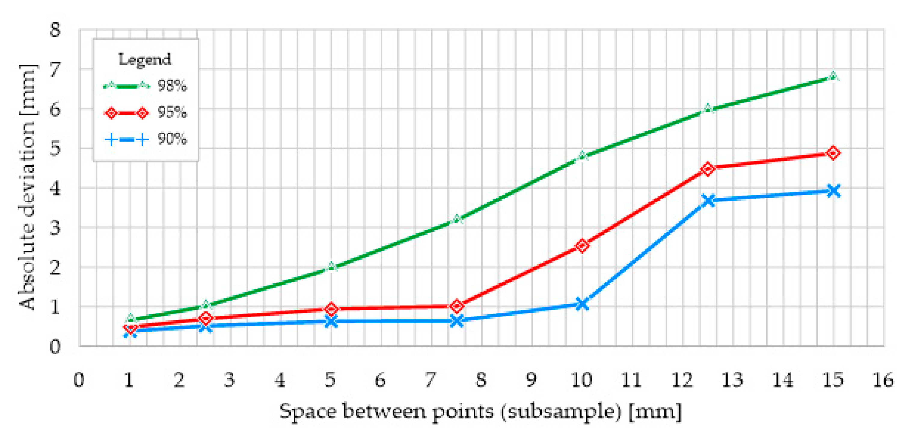
| Cumulated Absolute | 1 mm | 2.5 mm | 5 mm | 7.5 mm | 10 mm | 12.5 mm | 15 mm |
|---|---|---|---|---|---|---|---|
| 90% | 0.38 | 0.51 | 0.63 | 0.64 | 1.07 | 3.68 | 3.93 |
| 95% | 0.48 | 0.69 | 0.94 | 1.01 | 2.55 | 4.49 | 4.88 |
| 98% | 0.65 | 1.01 | 1.96 | 3.18 | 4.78 | 5.96 | 6.80 |
Publisher’s Note: MDPI stays neutral with regard to jurisdictional claims in published maps and institutional affiliations. |
© 2021 by the authors. Licensee MDPI, Basel, Switzerland. This article is an open access article distributed under the terms and conditions of the Creative Commons Attribution (CC BY) license (https://creativecommons.org/licenses/by/4.0/).
Share and Cite
Wałach, D.; Kaczmarczyk, G.P. Application of TLS Remote Sensing Data in the Analysis of the Load-Carrying Capacity of Structural Steel Elements. Remote Sens. 2021, 13, 2759. https://doi.org/10.3390/rs13142759
Wałach D, Kaczmarczyk GP. Application of TLS Remote Sensing Data in the Analysis of the Load-Carrying Capacity of Structural Steel Elements. Remote Sensing. 2021; 13(14):2759. https://doi.org/10.3390/rs13142759
Chicago/Turabian StyleWałach, Daniel, and Grzegorz Piotr Kaczmarczyk. 2021. "Application of TLS Remote Sensing Data in the Analysis of the Load-Carrying Capacity of Structural Steel Elements" Remote Sensing 13, no. 14: 2759. https://doi.org/10.3390/rs13142759