Article

DSDet: A Lightweight Densely Connected Sparsely Activated Detector for Ship Target Detection in High-Resolution SAR Images

1
National Laboratory of Radar Signal Processing, Xidian University, Xi’an 710071, China
2
Institute of Automation, Chinese Academy of Sciences, Beijing 100190, China
*
Author to whom correspondence should be addressed.
Remote Sens. 2021, 13(14), 2743; https://doi.org/10.3390/rs13142743
Submission received: 13 June 2021 / Revised: 5 July 2021 / Accepted: 9 July 2021 / Published: 13 July 2021

Abstract

:
Traditional constant false alarm rate (CFAR) based ship target detection methods do not work well in complex conditions, such as multi-scale situations or inshore ship detection. With the development of deep learning techniques, methods based on convolutional neural networks (CNN) have been applied to solve such issues and have demonstrated good performance. However, compared with optical datasets, the number of samples in SAR datasets is much smaller, thus limiting the detection performance. Moreover, most state-of-the-art CNN-based ship target detectors that focus on the detection performance ignore the computation complexity. To solve these issues, this paper proposes a lightweight densely connected sparsely activated detector (DSDet) for ship target detection. First, a style embedded ship sample data augmentation network (SEA) is constructed to augment the dataset. Then, a lightweight backbone utilizing a densely connected sparsely activated network (DSNet) is constructed, which achieves a balance between the performance and the computation complexity. Furthermore, based on the proposed backbone, a low-cost one-stage anchor-free detector is presented. Extensive experiments demonstrate that the proposed data augmentation approach can create hard SAR samples artificially. Moreover, utilizing the proposed data augmentation approach is shown to effectively improves the detection accuracy. Furthermore, the conducted experiments show that the proposed detector outperforms the state-of-the-art methods with the least parameters (0.7 M) and lowest computation complexity (3.7 GFLOPs).

Graphical Abstract

1. Introduction

Synthetic aperture radar (SAR) has the unique capability of earth observation in all-weather conditions, regardless of day and night, which gives it an important place in marine exploration [1,2,3,4,5]. As a multitude of spaceborne SAR sensor platforms (e.g., RADARSAT-2, TerraSAR-X [6], and GF-III) are put into operation, high-resolution SAR images are no longer difficult acquire [7,8], which promotes the use of SAR imaging in ocean monitoring.
Marine ship target detection in SAR images plays an important role in sustainable fishing, marine ecosystem protection, and military target strikes. The traditional SAR ship target detection framework can be mainly divided into four stages: land-sea segmentation, preprocessing, prescreening, and discrimination [9,10], for which researchers have developed a variety of methods. Since the detection for land areas results in a large number of false alarms, and since dealing with these false alarms greatly increases the burden on the system, land-sea segmentation serves as an essential pretreatment. For most of the general land-sea segmentation methods, such as geographic information system (GIS), snake model [11], and Otsu [12,13], prior knowledge as well as various handcraft features are used to segment the SAR image. In order to improve detection performance, researchers have proposed preprocessing methods to enhance the ship targets’ characteristics. Weighted information entropy [14] and visual attention mechanism [15,16] serve as two such methods.
Among the four detection stages, prescreening is the crucial step [17] whose primary purpose is to locate targets. Actually, many ship detection methods only contain this step [18]. Among existing detection methods, CFAR based methods [19] have been widely investigated [20,21,22,23,24,25]. This type of method determines the detection threshold based on a pre-established clutter statistical model, which has the characteristic of constant false alarms [26,27]. These statistical methods strongly rely on the statistical distribution of sea clutters. However, such models are easily affected by ocean currents, climate, and imaging systems, which reduces the robustness of CFAR [10]. To alleviate the sea clutter model’s mismatch risk, researchers have explored many clutter distribution models. However, with the increasing complexity of the models, parameter estimation becomes a challenge and even constrains the practical application of CFAR technology.
Discrimination is used by an operator to eliminate non-ship targets based on the classification features extracted in the prescreening areas. Length-width ratio [10], geometric shape, scale-invariant feature transform (SIFT) [28], and histogram of oriented gradient (HOG) [29] are the commonly used features. However, these handcraft features do not work well in complex inshore areas.
In recent years, due to the significant strides in deep learning in the field of computer vision, i.e., image classification [30], object detection [31,32], and image segmentation [33,34], researchers try to introduce deep learning methods in ship detection. Deep learning methods detect the position of ships by spontaneously learning the ships’ characteristics through a labeled dataset. They do not require land-sea segmentation and have demonstrated satisfactory effects in multi-scale and inshore ship detection tasks. Faster R-CNN [35] and You Only Look Once (YOLOv1-v3) [36,37,38] are two classic algorithms that represent the two-stage and one-stage detectors, respectively, laying the foundation for the basic architecture for current mainstream detection algorithms. Recently, many SAR ship detection methods based on these architectures have been proposed [39,40]. A dense network was constructed by Jiao et al. [41] to extract additional features at different levels. Additionally, Cui et al. [42] added an attention network in a feature pyramid to solve the problem of multi-scale ship detection. Wang et al. [43] improved the original SSD method by introducing an angle regression branch and aggregating semantic information. Moreover, Lin et al. [44] improved the Faster R-CNN and concatenated three-level features to obtain multi-scale feature maps. Yang et al. [45] detected ship targets in four different level features. In addition, to further improve the detection performance and address the influence of multi-scale and complex backgrounds, Zhao et al. [46] employed receptive fields block and the convolutional block attention module (CBAM) [47] to build a top-down feature pyramid. Furthermore, Fu et al. [48] added level-based attention and spatial-based attention networks into the feature pyramid network to enhance the feature extraction ability of the detector.
Although current CNN-based ship detection methods have attained compelling results, certain problems still require further elucidation. Recent deep learning-based ship detectors mainly focus on detection accuracy. Good performance always comes with a larger number of parameters as well as a heavy computational burden. However, few studies focus on reducing the computation complexity. Accordingly, how to balance the detection performance and the computation complexity is a problem.
Moreover, most recent approaches rely on pre-defined anchor boxes, which makes them achieve adequate performances [33,39]. However, it should be noted that the anchor-based detectors suffer from some drawbacks. First, many hyper-parameters are introduced when designing these anchor boxes. To achieve good detection performance, these pre-defined anchors require complex manual calibration of the hyper-parameters. Second, ship targets have large-scale variations (e.g., size and orientation). To adapt to this variation, a few different pre-defined anchors should be designed for the detectors. However, it can be observed that the orientations of ship targets are arbitrary, and the corresponding bounding boxes also have enormous change. The pre-defined anchors cannot effectively cover this change. Meanwhile, to acquire better performance, anchors are densely placed on the image. Considering the sparsity of the ships, redundant pre-defined anchors will increase the computational burden. Therefore, anchor-free methods may be potentially better in ship detection tasks, which directly determine the geometric shape by extracting the semantic information of the target.
Furthermore, as a data-hungry approach, deep learning demands a large number of training samples to ensure its performance and generalization ability. Compared with optical datasets, the number of samples in SAR datasets is much smaller, which limits the detection performance. Data augmentation is an efficient way to address these issues. Crop, rotation, saturation, bilateral blurring, MixUp, CutMix and Mosaic are the representative conventional data augmentation methods. However, such methods cannot improve the detection performance to a satisfactory extent. Many novel data augmentation methods have been developed to improve the SAR classification performance [49,50,51]. However, similar studies in the field of SAR ship detection have hardly been conducted.
In response to the aforementioned problems, this paper proposes DSDet for ship target detection in high-resolution SAR images, as illustrated in Figure 1. First, a style embedded ship sample data augmentation network (SEA) is constructed to augment the dataset. Then, a lightweight densely connected sparsely activated network (DSNet) is devised as the backbone. Furthermore, based on the proposed backbone, a low-cost one-stage anchor-free detector is presented, achieving a balance between performance and computation complexity.
The proposed detection framework provides the following contributions:
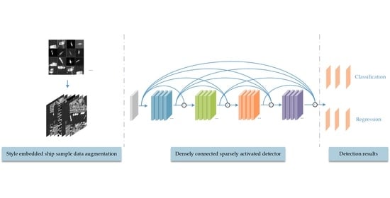
  • A new SAR ship sample data augmentation framework based on generative adversarial network (GAN) is proposed, which can purposefully generate abundant hard samples, simulate various hard situations in marine areas, and improve detection performance. Additionally, as data augmentation is only applied in the training stage, it does not incur extra inference costs;
  • A cross-dimension attention style embedded ship sample generator, as well as a max-patch discriminator, are constructed;
  • A lightweight densely connected sparsely activated detector is constructed, which achieves a competitive performance among state-of-the-art detection methods;
  • The proposed method is proposal-free and anchor-free, thereby eliminating the complicated computation of the intersection over union (IoU) between the anchor boxes and ground truth boxes during training. As a result, this method is also completely free of the hyper-parameters related to anchor boxes, which improves its flexibility compared to its anchor-based counterparts.
The remainder of this paper is organized according to the following manner. The style embedded ship sample data augmentation is introduced in Section 2. Section 3 presents a detailed description of the lightweight densely connected sparsely activated detection method. Then, the comparative experimental results with real SAR images are provided and analyzed in Section 4. Finally, the paper’s conclusion is given in Section 5.

2. Style Embedded Ship Sample Data Network

Usually, a conventional object detector is trained offline. Therefore, researchers always prefer to take this advantage by developing better training methods to make the object detector attain better accuracy without increasing the inference cost [52]. Conventional data augmentation methods crop, rotate, or blur the original sample, whereas hard samples are not augmented. They still cannot be detected efficiently. To solve this issue, this section constructs a novel ship sample augmentation method. The concept of this approach is to create hard samples artificially and purposefully. Specifically, ship slices are embedded into SAR images to simulate the various hard situations encountered during detection. However, simply embedding the ship slices into SAR images cannot simulate a real SAR image as the embedded slices are not in harmony with the surrounding environment. To address this problem, a style embedded ship sample data augmentation network is constructed. Figure 2 shows the flow chart of the proposed sample augmentation method.
Given a real SAR image I , the pre-prepared ship slice images are embedded into I so as to obtain the embedded image I e . To improve the generated results, this paper proposed a two-channel (original SAR image and embedded SAR image) input mechanical. Next, the ship mask M is made, indicating the regions where the embedded ships are located. Mask M is only used in the training stage to help improve the final result. The purpose of the ship sample augmentation method is to train a model that reconstructs I g to be closed to the real SAR image. To achieve this goal, a GAN framework is utilized. As shown in Figure 2, the method consists of two parts: generator G and discriminator D.
Specifically, the real SAR image and the embedded SAR image are treated as positive and negative samples, respectively. On the one hand, the discriminator is trained to distinguish positive images from negative images. On the other hand, the generator is expected to produce a harmonized image that can fool the discriminator. The discriminator and generator improve the performance during the confrontation. Details are described as follows.

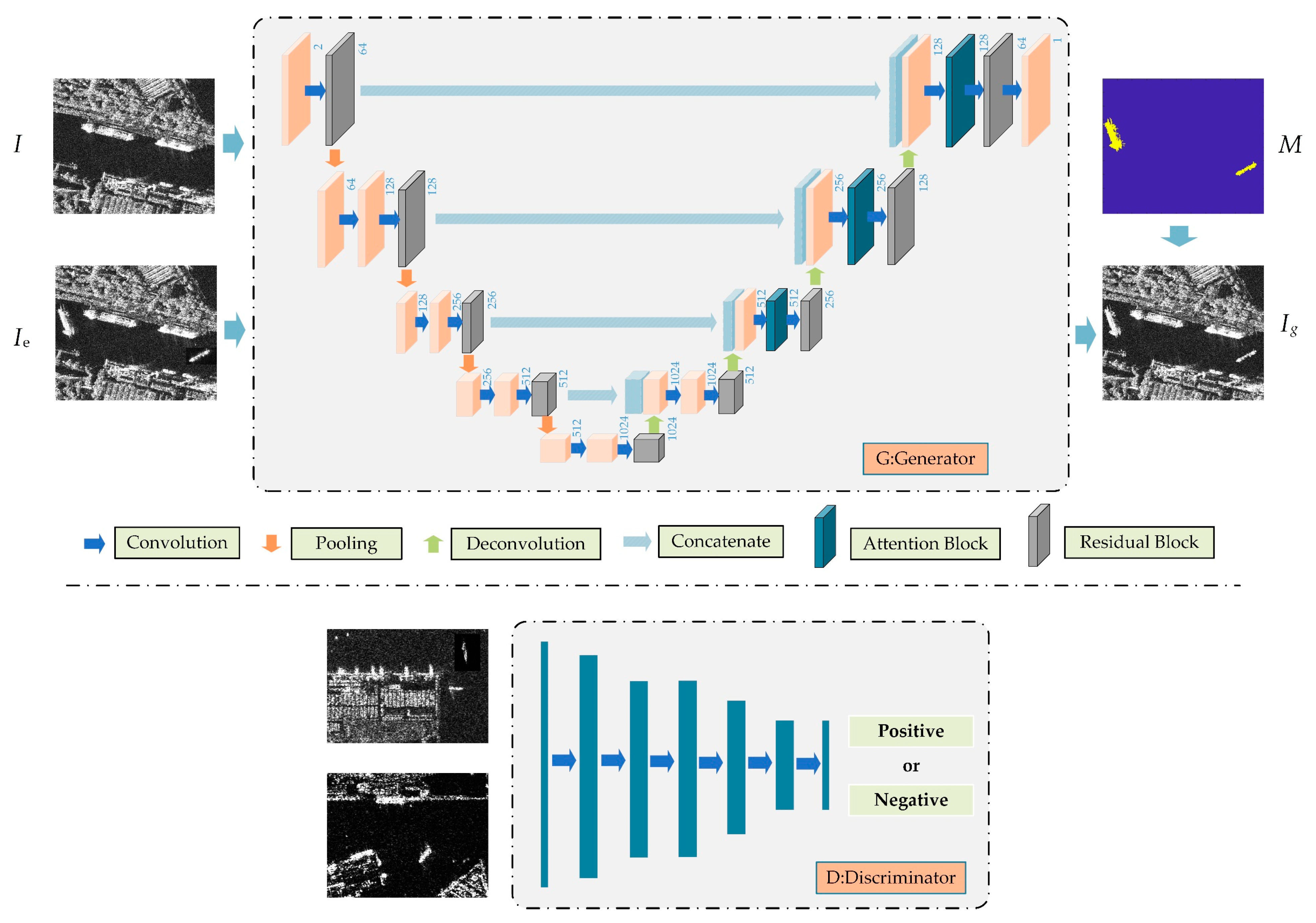
2.1. Cross-Dimension Attention Style Embedded Ship Sample Generator

Based on U-Net [53], a cross-dimension attention style embedded ship sample generator is constructed in this section. The architecture of the network is shown in Figure 3. It follows the framework of the encoder-decoder. The encoder module utilizes classic convolution to extract features, while the decoder module utilizes deconvolution to expand the spatial resolution of the features and concatenates the same stage features from the encoder module. The concatenation operator in U-Net realizes the interaction between shallow features and deep features. Notably, the importance of features in the shallow and deep levels is different [54], and we hope the generator pays more attention to the embedded ships. As a result, to aggregate the features and improve the generated result, attention block and residual block are inserted, as depicted in Figure 2. The details of the network are shown in Figure 3.
The cross-dimension aggregation attention module is realized by capturing the interaction between ( C , W ) , ( C , H ) and ( H , W ) dimensions of the input features, respectively [54]. Figure 4 shows the structure of this module. The inputted feature map F i n C × H × W goes through three branches. Taking the second branch as an example, the input feature F i n C × H × W is rotated through 90° clockwise along the W axis. F 2 H × W × C is the rotated feature. Then, adaptive pooling is applied to preserve a rich representation of the feature while simultaneously shrinking its depth, which is expressed as:
F 2 p o o l 2 × W × C = [ M a x p o o l ( F i n ) 2 , A v g p o o l ( F i n ) 2 ]
Next, the pooled feature is processed through a standard convolution layer and a sigmoid activation layer. After this step, the intermediate output is subsequently rotated through 90° anticlockwise along the W axis to obtain F 2 C × 1 × W . Similarly, the output of the other two branches are F 1 and F 3 .
Finally, the residual module is utilized to obtain the aggregation output, shown as follow:
F o u t = { A v e r a g e ( F i n F 1 + F i n F 2 + F i n F 3 ) }
The generated image I g = G ( I , I e ) is enforced to be close to the real SAR image via:
L p i x e l = I I g 2 | ( r e g i o n = ! M ) + I e I g 2 | ( r e g i o n = M )
where · 2 is the L2-norm. r e g i o n = M represents the region where the embedded ships are located. r e g i o n = ! M represents the region without the ships. It should be noted that mask M is only used in the training stage to help improve the final result.

2.2. Max-Patch Discriminator

Discriminator D is designed to help generator G generate more plausible SAR images. In this section, a max-patch discriminator is constructed, which consists of seven convolution layers. After each convolution layer, LeakyReLU activation and instance normalization layers are applied. Sigmoid activation is placed after the last layer. The architecture of the network is shown in Table 1.
Voting is used to determine whether the input is positive or negative. Specifically, the response values of the network are sorted, then the max N values are selected to calculate the average, which is taken as the final discrimination result. N is set as 25 in this paper.
Cross entropy is leveraged for training, which is given by:
L D = log ( D ( I ) ) log ( 1 D ( G ( I , I e ) ) )
L G = log ( D ( G ( I , I e ) ) )
where D and G denote the discriminator and the generator, respectively. D ( ) and G ( ) are their outputs. L D and L G represent the discrimination quality loss and generation quality loss, respectively.
The overall loss function of the training process is defined as a weighted sum of the losses, which is expressed as:
G l o s s = argmin ( λ 1 L p i x e l + λ 2 L G )
D l o s s = argmin ( L D )
where λ 1 and λ 2 are set as 1 in this paper. G l o s s and D l o s s represent the generator loss and discriminator loss, respectively.

3. Lightweight Densely Connected Sparsely Activated Detector

In this section, firstly, the convolution module is introduced. Then, the lightweight backbone network is constructed. Finally, the detection framework is described in detail.

3.1. Convolution Module

The conventional convolution neural network is widely used in modern network architectures, such as ResNet [55], GoogLeNet [56], and Darknet [36,37,38], which is used by most of the object detectors in extracting features. However, good feature extraction ability is always associated with a large number of parameters and high computational complexity. The group convolution and the depthwise convolution are two architectures that reduce the computational complexity by changing the convolution density between all channels. The architectures of the conventional convolution, the group convolution and the depthwise convolution are shown in Figure 5.
According to Figure 5a, the conventional convolution’s filter should process each feature map to generate a new layer. For Figure 5a, the conventional convolution has 8 × 4 = 32 convolution operators. Compared with the conventional convolution, the group convolution has a lower computational complexity. In regard to Figure 5b, the group convolution has 4 × 4 = 16 convolution operators. The depthwise convolution only needs to convolute one input channel. Hence, for Figure 5c, the depthwise convolution merely has 8 × 1 = 8 convolution operators. To reduce the computational complexity, the group convolution and the depthwise convolution are adopted to construct the backbone.

3.2. The Architecture of DSNet Backbone

Target detection requires a wealth of information. In deep convolution networks, the degree of information abundance varies from low to high, and the special resolution varies from high to low. With the increases of network depth and decrease of spatial resolution, a single layer cannot provide enough information. How to better integrate the information between different stages and blocks of the network is a problem that needs further consideration.
Reusing features in deep networks via dense connection is an effective way to achieve high computational efficiency [57]. The counter-intuitive effect of the dense connected mode is that it requires fewer parameters than traditional convolutional neural networks as it does not need to relearn redundant features. A densely connected mode can improve the flow of information through the network, which makes training easier. Each layer has a direct path from the loss function and the input information directly to the gradient, which allows for deeper supervision. Furthermore, a dense connection has a regularization effect, which reduces overfitting on smaller training data sets [57].
Since a densely connected model reuses shallow features, as the network depth increases, the number of network layers increases and the computational complexity also increases significantly. To solve such a problem DSNet is constructed, which adopts a densely connected model to reuse shallow features and utilizes sparse convolution (e.g., group convolution and depthwise convolution) networks to activate the feature layers. Moreover, the output channels of each convolutional layer are shuffled to ensure communication between different groups. The sparse activate module of this architecture is shown in Figure 6.
Figure 7 shows the architecture of DSNet. H S A ( · ) is the sparse active module. In addition, the number of pixels occupied by the ship target in SAR image is usually relatively small. Hence, two networks with different spatial resolutions refer to as DSNet 1.0× and DSNet 2.0× are constructed, respectively. Details of the DSNet can be found in Appendix A.

3.3. The Location of Bounding Box

The geometric shape of the ship target is a long ellipse, and the orientation is arbitrary. Therefore, the corresponding bounding boxes undergo a large change (e.g., extreme aspect ratios). Figure 8 shows the typical SAR ship images. The design of the anchors is empirical, which cannot fully describe the shape of ship targets. Although the regression branch can slightly amend the anchor box, the anchor-based framework still has lower flexibility, and ships with a peculiar shape may be lost. Therefore, an anchor-free framework could be more suitable for ship detection.
Depending on how to encode the bounding box’s location, anchor-free methods can be divided into point-grouping detectors and point-vector detectors [58]. Point-grouping detectors use two individual branches to detect key points and their offset maps. These key points can then be grouped together by the offset maps. The point-vector detectors determine the bounding box of targets by the key point and its vector. The encoded location of the bounding box is illustrated in Figure 9.
Considering point-grouping methods need to cluster the detected corner points, which suffer from mismatching in the case of densely distributed conditions [57], the point-vector bounding box is accepted in this paper.
Anchor-based detectors use the pixel position on the input image as the anchor’s center point to regress the bounding box, amending the preset anchors. In contrast, DSDet regards the locations of bounding boxes as training samples instead of anchor boxes and directly regresses the bounding box at the location. All the points in the ground truth boxes are regarded as positive samples. This is different from anchor-based methods which only select the high IoU score anchor boxes as the positive samples.
The predicted bounding box is encoded by a four-dimension (4-D) vector ( x t , y t , x b , y b ) . Here ( x t , y t ) and ( x b , y b ) denote the coordinates of the left-top and right-bottom corners of the bounding box. The 4-D training target v = ( l , t , r , b ) is utilized to regress the bounding box, which is calculated by:
l = x x t , t = y y t , r = x b y ,   b = y b y .
where ( x , y ) is the coordinate of the pixel point.

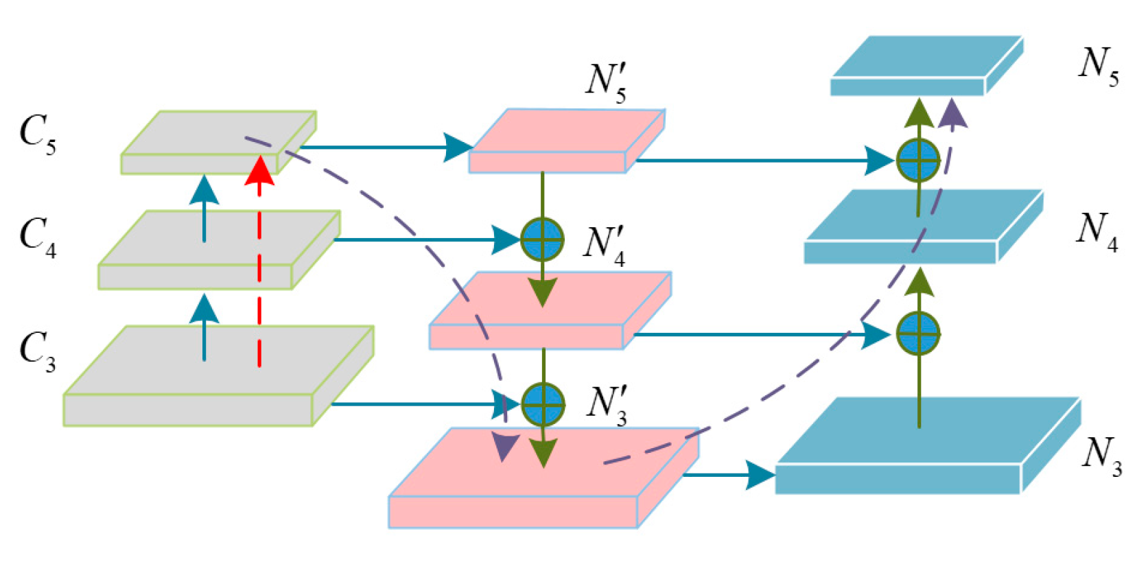
3.4. Deep Feature Fusion Pyramid

Early methods only employed one stage feature map to detect targets. High-level feature maps have large receptive fields and can capture richer semantic information. However, it is hard for them to detect small-scale targets due to their low spatial resolution. In contrast, low-level feature maps have richer spatial information but provide less semantic information, enabling high localization accuracy but worse classification performance. This imbalance between different levels reduces multi-scale ship detection performance. Therefore, it is a natural choice to construct a feature pyramid using different levels of features to detect targets. Furthermore, different level features capture different context information. The important features of targets may not distribute in a single level. Hence, features at different levels should be appropriately fused.
Based on the considerations above, this paper introduces a deep feature fusion pyramid, which aims to let small proposals access the fusion pyramid exploiting more useful contextual information and large proposals acquire rich spatial information.
The structure is illustrated in Figure 10, for which DSNet is taken as the backbone of the detector. The output of stages 3–5 are utilized to detect targets. As shown in Figure 1, the output of stages 3–5 in the network is defined as { C 3 , C 4 , C 5 } . { N 3 , N 4 , N 5 } denotes the feature levels generated by the feature fusion pyramid. The augmented path starts from the lowest level C 3 and gradually approaches C 5 . From C 3 to C 5 , the spatial size is gradually down-sampled with a factor of 2.
In order to reduce the computational complexity, the feature fusion pyramid is simplified by using fewer convolution operations. In particular, for feature level 3~4, feature map C i first passes through a 1 × 1 convolutional layer. Then, each element in this layer is added with the up-sampled high-level feature to obtain an intermediate feature N i . Finally, intermediate feature N i is processed via down-top path to generate N i . This process is summarized as:
N i = { C o n v 1 × 1 ( C i ) + u p _ s a m p l e d ( N i + 1 ) } , ( i = 3 , 4 ) N 5 = { C o n v 1 × 1 ( C 5 ) ) } , N i = { N i + d o w n _ s a m p l e d ( N i 1 ) } , ( i = 4 , 5 ) N 3 = { N 3 } .

3.5. Loss Function

At the end of the detection, a non-maximum suppression (NMS) process is adopted to select the position of the targets. NMS process ranks all detection results according to their classification confidence and selects the highest classification score bounding box as the final position of the targets. This process has the risk that low classification confidence but high-quality bounding boxes may be filtered. To address this issue, generalized focal loss [59] is introduced in the loss function. The total loss function is constructed as:
( { q x , y } , { b x , y } ) = 1 N p o s x , y q u a ( q x , y , q x , y * ) + 1 N p o s x , y r e g ( b x , y , b x , y * ) .
The training loss function consists of two parts: q u a and r e g . They represent the quality loss and regression loss, respectively. Here, N p o s is the number of positive samples, while q x , y and q x , y * denote the quality prediction score and the ground truth label, respectively. The ground truth label q x , y * represents the IoU score of the regressed box. The quality loss adopts quality focal loss [59] to measure the difference between the predicted quality and the ground truth label. denotes the positive region. b x , y and b x , y * denote the predicted location and the ground truth box.
q u a ( q x , y , q x , y * ) = ( q x , y * q x , y ) β ( ( 1 q x , y * ) log ( 1 q x , y ) + q x , y * log ( q x , y ) )
where β is set as 2.
Distance-IoU loss [60] and distribution focal loss [59] are adopted to measure the distance between the predicted box and the ground truth box, which are calculated by:
r e g ( b x , y , b x , y * ) = λ 3 D I o U + λ 4 D F L
D I o U = 1 I o U + | C B B g t | | C |
I o U = | B B g t | | B B g t |
where B and B g t represent the predicted box and ground the truth box. C is the smallest box covering B and B g t . λ 3 and λ 4 are set as 0.3 and 2, respectively.
The relative offsets from the location to the four sides of a bounding box are adopted as the regression targets, as shown in Figure 9c. g is the regressed label. Given the range of label g with minimum g 0 and maximum g n ( g 0 < g < g n ), the range [ g 0 , g n ] is divided into a set { g 0 , g 1 , , g n } . The estimated regression value g ^ can be calculated by:
g ^ = i = 0 n P ( g i ) g i , i = 0 n P ( g i ) = 1
P ( ) can be easily implemented through a SoftMax S ( ) layer consisting of n + 1 units, with P ( g i ) being denoted as S i for simplicity. n is set as 7, and the interval is 1. Then, the loss function can be expressed as follow:
D F L ( S i , S i + 1 ) = ( ( g i + 1 g ) log ( S i ) + ( g g i ) log ( S i + 1 ) )
where g i and g i + 1 are the nearest to the label g ( g i < g < g i + 1 ).

4. Experiments and Discussions

In this section, experiments with real SAR images are carried out to assess the competence of the proposed method. In the following experiments, the dataset and evaluation metrics are introduced first. Then, the performance of the ship sample augmentation method is illustrated. Additionally, detailed experiments of the proposed lightweight detection network are conducted.

4.1. Dataset

The SSDD [61] and HRSID dataset [8] are selected to evaluate the proposed method. SSDD is the first public SAR ship detection dataset, which is mainly provided by Radarsat-2, TerraSAR-X, and Sentinel-1 sensors, taken in Yantai, China, and Visakhapatnam, India, with the resolution of 1 m–15 m. It contains a large number of ship targets in the sea and coastal areas. In SSDD, there are 1160 images and 2456 ships with an average of 2.12 ships per image. The training subset contains 928 images, and the test subset contains 232 images.
HRSID is a large SAR ship detection dataset published recently. It contains multi-scale ships labeled with bounding box in various environments, including different scenes, sensor types and polarization modes. Statistically, there are 5604 cropped SAR images and 16,951 annotated ships in HRSID. The average number of ships per image is 3. Table 2 shows the main parameters of SSDD and HRSID.
In the data augmentation experiment, half of the training data in SSDD are randomly selected as positive samples and the other half are used to embed ship slices to train the generator. The training epoch is 50, and the optimizer is Adam who has a learning rate of 0.0004. Beta 1 and beta 2 are set as 0.9 and 0.999, respectively.
The detector model is pre-trained on the COCO dataset [62]. In the following experiment, the training epoch is 100, and the stochastic gradient descent (SGD) algorithm is used as the optimizer. The initial learning rate is set as 0.1, and it decays in the 50th and 75th, adopting 0.01 and 0.001, respectively.

4.2. Evaluation Criteria

In order to quantitatively evaluate the detection performance of the network, the following evaluation criteria are used.
The detection precision and recall are the basic performance evaluation criteria of the traditional detection algorithms. The definitions are expressed by:
P r e c i s i o n = T P T P + F P
R e c a l l = T P T P + F N
where TP is the number of truly detected ships, FP is the number of backgrounds detected as ships, and FN represents the number of ships detected as the background. The true detected ship is defined as the target whose IoU between its bounding box and ground truth is higher than 0.5.
High precision and recall rate is difficult to meet at the same time, hence, AP shown in Equation (19) is adopted to evaluate the overall performance of the detection methods.
A P = 0 1 P ( R ) d R
where P denotes precision, and R represents recall. AP is the primary challenge metric with the calculation of average IoU, which has ten IoU thresholds distributed from 0.5 to 0.95 with a step of 0.05. AP50 is the AP score when the IoU threshold is chosen as 0.5. Similarly, AP75 is the AP score when the IoU threshold is chosen as 0.75. Aps, APm, and APl denote the objects with small (area < 32 2 pixels), medium ( 32 2 < area < 64 2 pixels), and large ( 64 2 < area) size.

4.3. The Performance of the Ship Sample Augmentation Method

4.3.1. The Generated Results of the Proposed Method

Figure 11 shows the generation performance of the proposed sample augmentation method. Figure 11a shows the original SAR images; Figure 11b shows the embedded SAR images that simulate the various states of ship targets in the inshore and offshore areas; Figure 11c illustrates the generated images. Evidently, the embedded ships are very inconsistent with the surrounding environment (as shown in Figure 11b). On the contrary, ships in the generated images are observed to be consistent with the surrounding environment, which demonstrates the effectiveness of the proposed augmentation method.

4.3.2. The Comparison of the Generated Results between the Proposed Method and U-Net

In order to verify the effectiveness of the proposed generator’s network, the proposed network is compared with U-Net. Figure 12a shows the embedded SAR images, while Figure 12b depicts the results of U-Net and Figure 12c illustrates the results of the proposed method. According to Figure 12, the proposed network has a superior generation performance than U-Net. It can be observed that the proposed method not only preserves the details of the ship targets but also integrates the targets and the background well, which demonstrates the outperformance of the proposed method.

4.3.3. The Effectiveness of the Proposed Two-Channel Input Mechanical

To verify the effectiveness of the proposed two-channel input mechanical, an experiment is conducted. Figure 13 shows the results of the single-channel (only the embedded SAR image) input and two-channel input. Evidently, the results of the two-channel input exhibit better performance. The reason is that the two-channel input mechanical increases the available information of the generator so that the generator can easily find the embedded targets from the comparison and make it harmonious with the surrounding environment. On the contrary, the single-channel input mechanical is unable to specify the target areas for the generator, which increases the learning difficulty of the generator.

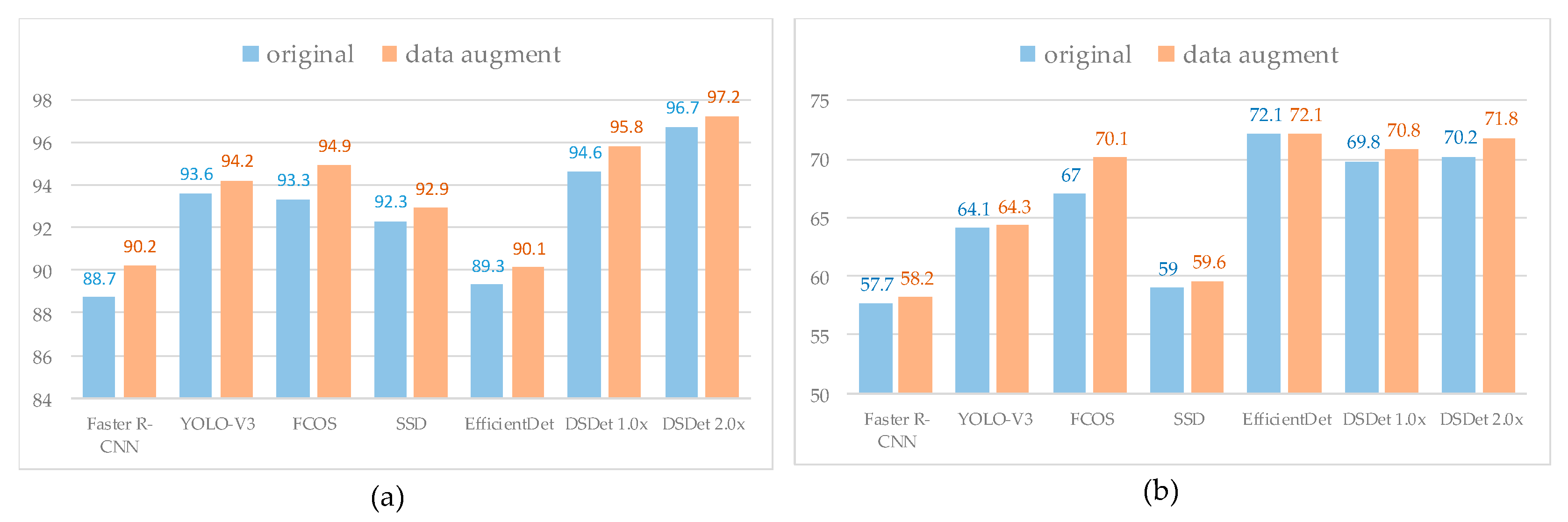
4.4. The Results of Ship Detection on SSDD

4.4.1. Accuracy

To evaluate the performance of the proposed method, comparison experiments on Faster R-CNN [35], YOLO-V3 [38], FCOS [58], SSD [63], and EfficientDet [64] are conducted. The comparison results of the detection performance are quantitatively shown in Table 3. The results in bold signify the best result of the corresponding index. It can be observed from Table 3 that the AP, AP50, AP75, APs, APm, and APl of DSNet with backbone DSNet 1.0× are 59.8%, 94.6%, 69.8%, 55.0%, 66.9%, and 61.8%, respectively. Meanwhile, the AP, AP50, AP75, APs, APm, and APl of DSNet with backbone DSNet 2.0× are found to be 60.5%, 96.7%, 70.2%, 56.3%, 68.1%, and 58.9%, respectively. Compared with DSNet 1.0×, DSNet 2.0× exhibits better performance, which demonstrates that using features with high spatial resolution can improve the detection performance.
Without considering the data augmentation method, the proposed DSDet (DSNet 2.0×) obtains the highest performance in the AP, AP50, and APs, garnering a 1.2%, 3.1%, and 1.7% improvement compared to the highest performance of the comparison methods. As for AP75 and APm, the performance of the proposed DSDet (DSNet 2.0×) is noted to be slightly lower than the highest performance of the comparison method, with a rather small gap. In terms of the overall performance, the proposed method demonstrates obvious advantages. Moreover, when using the proposed data augmentation approach, the proposed method exhibits obvious superior performance in almost all evaluation criteria.
Figure 14 shows the effect of the proposed data augmentation method on AP50 and AP75. The proposed data augmentation approach gains 1.5%, 0.6%, 1.6%, 6.3%, 0.6%, 0.8%, 1.2% and 0.5% in terms of AP50 for Faster R-CNN, YOLO-V3, FCOS, SSD, EfficientDet, DSNet 1.0×, and DSNet 2.0×, respectively. Moreover, the AP75 values of Faster R-CNN, YOLO-V3, FCOS, SSD, DSNet 1.0×, and DSNet 2.0× also gain 0.5%, 0.2%, 3.1%, 0.6%, 1.0%, 0.8% and 1.6% improvement, respectively. Actually, the AP, APs, APm, and APl performances are also significantly improved, which means the small, medium, and large targets’ detection accuracies are also improved, as shown in Table 3. Evidently, the proposed data augmentation approach can effectively improve the detection performance.

4.4.2. Computational Complexity

The visualization results under different metrics are given in Figure 15 to illustrate the complexity and accuracy of the proposed method. Here, compared with the comparison methods, the proposed detector has the least number of parameters (0.7 M), while the number of parameters in Faster R-CNN, YOLO-V3, FCOS, SSD, EfficientDet are 60.3 M, 61.5 M, 32.1 M, 23.8 M, and 20.5 M, respectively. The second smallest detector EfficientDet is still larger than the proposed DSDet 1.0× by 29-fold. This signifies that the weight of the proposed method is far lighter than all other methods. Besides, the proposed detector receives the lowest computational complexity (3.7 GFLOPs, 14.3 GFLOP), while that of Faster R-CNN, YOLO-V3, FCOS, SSD, EfficientDet are 134.4 GFLOPs, 87.7 GFLOPs, 121.1 GFLOPs, 127.8 GFLOPs, 107.5 GFLOPs, respectively. The second-lightest YOLO-V3 is still heavier than the proposed DSDet 1.0× by 24-fold. Moreover, the accuracy of the proposed detector is also the highest. In general, the above results demonstrate that, compared with the comparison methods, the proposed detector has the highest accuracy, lowest computational complexity, and least number of parameters.

4.5. Results of Ship Detection on HRSID

To verify the robustness and migration capacity of the proposed detector in different datasets, the detection performance of the proposed detector is further tested in HRSID dataset. HRSID provides abundant baselines. We use these baselines to verify the detection performance. Table 4 shows the comparison of different detectors on the HRSID dataset. According to Table 4, compared with other baselines, HRSDNet with backbone HRFPN-W40 has the best overall performance, whose AP, AP50, AP75, APs, APm, and APl criteria are 69.4%, 89.3%, 79.8%, 70.3%, 71.1% and 28.9%, respectively. The detection accuracy of RetinaNet with backbone ResNet-100 + FPN is noted to be much lower than the other baselines. The AP, AP50, AP75, APs, APm and APl of RetinaNet with backbone ResNet-100 + FPN are 59.8%, 84.8%, 67.2%, 60.4%, 62.7%, and 26.5%, respectively.
Additionally, the AP, AP50, AP75, APs, APm and APl of DSNet with backbone DSNet 2.0× are found to be 60.5%, 90.7%, 74.6%, 66.8%, 64.0%, and 7.6%, respectively. The performance of the proposed DSDet was slightly lower than the highest performance baseline HRSDNet. Despite the slight sacrifice in accuracy, the model parameter and model size of the proposed detector is rather small, which are the 1/130.2 and 1/130 of the HRSDNet with backbone HRFPN-W40. In terms of the model parameter and model size, the proposed detector outperforms all comparison detectors by a large margin. Moreover, the proposed detector also attains the highest accuracy in AP50. In general, the proposed detector has a competitive overall performance with the least number of parameters and model size among the state-of-the-art detectors.

5. Conclusions

Compared with optical datasets, the number of samples in SAR datasets is much smaller. Moreover, most state-of-the-art CNN-based ship target detectors are computationally expensive. To address these issues, this paper proposes a SAR ship sample data augmentation method as well as a lightweight densely connected sparsely activated detector. The proposed sample data augmentation framework can purposefully generate abundant hard samples, simulate various hard situations in marine areas, and improve detection performance. In addition, dense connection and sparse convolution modules are utilized to construct the backbone. Based on the proposed backbone, a low-cost one-stage anchor-free detector is presented. The validity of the proposed method is then confirmed on the public datasets SSDD and HRSID. The experimental results indicated that the proposed data augmentation method can evidently improve the detection performance. Benefiting from the lightweight design of the detection network, the proposed detector achieves competitive performance compared to other state-of-the-art detectors with the least number of parameters and lowest computation complexity.
Ship instance segmentation in SAR images under complex sea conditions is an important research topic in the field of detection. The proposed lightweight detector can be remolded to construct a low-cost SAR ship instance segmentation method. Consequently, our future studies will focus on the ship instance segmentation for high-resolution SAR images.

Author Contributions

Conceptualization, K.S., Y.L. and M.X.; methodology, K.S.; software, K.S.; validation, K.S., X.M.; formal analysis, Y.H.; writing—original draft preparation, K.S.; writing—review and editing, Y.H.; funding acquisition, Y.L. All authors have read and agreed to the published version of the manuscript.

Funding

This work was supported by the National Natural Science Foundation of China under Grant 61971326.

Data Availability Statement

No new data were created or analyzed in this study. Data sharing is not applicable to this article.

Acknowledgments

We owe many thanks to the authors of HRSID and SSDD for providing the SAR image dataset. We would like to thank the anonymous reviewers for their valuable comments to improve the paper quality.

Conflicts of Interest

The authors declare no conflict of interest.

Appendix A

Table A1. The structure of the DSNet 1.0×.
StageInput SizeOperatorOutput SizeOutput Channel Number
{Kernel size, Convolution type, Channel number, Group number, Stride}
1 512 × 512 { 3 × 3 ,   Conv ,   12 ,   1 ,   2 } × 1 256 × 256 12
2 256 × 256 { 1 × 1 ,   GConv , 6 , 6 , 2 3 × 3 ,   DWConv , 6 , 6 , 1 1 × 1 ,   Conv , 6 , 1 , 1 } × 1 128 × 128 18
{ 1 × 1 ,   GConv , 6 , 6 , 1 3 × 3 ,   DWConv , 6 , 6 , 1 1 × 1 ,   Conv , 6 , 1 , 1 } × 1 24
3 128 × 128 { 1 × 1 ,   GConv , 12 , 6 , 2 3 × 3 ,   DWConv , 12 , 12 , 1 1 × 1 ,   Conv , 12 , 1 , 1 } × 1 64 × 64 36
{ 1 × 1 ,   GConv , 12 , 6 , 1 3 × 3 ,   DWConv , 12 , 12 , 1 1 × 1 ,   Conv , 12 , 1 , 1 } × 2 60
{ 1 × 1 ,   GConv , 24 , 6 , 1 3 × 3 ,   DWConv , 24 , 24 , 1 1 × 1 ,   Conv , 24 , 1 , 1 } × 2 108
{ 1 × 1 ,   GConv , 36 6 , 1 3 × 3 ,   DWConv , 36 36 1 1 × 1 ,   Conv , 36 1 , 1 } × 2 180
{ 1 × 1 ,   GConv , 48 6 , 1 3 × 3 ,   DWConv , 48 48 1 1 × 1 ,   Conv , 48 1 , 1 } × 1 228
{ 1 × 1 ,   GConv , 192 6 , 1 3 × 3 ,   DWConv , 48 48 1 1 × 1 ,   Conv , 48 1 , 1 } × 1 276
{ 1 × 1 ,   GConv , 60 , 6 , 1 3 × 3 ,   DWConv , 60 , 60 , 1 1 × 1 ,   Conv , 60 , 1 , 1 } × 1 336
4 64 × 64 { 1 × 1 ,   GConv , 96 , 6 , 2 3 × 3 ,   GConv , 24 , 24 , 1 1 × 1 ,   Conv , 24 , 1 , 1 } × 1 32 × 32 360
{ 1 × 1 ,   GConv , 96 , 6 , 1 3 × 3 ,   GConv , 24 , 24 , 1 1 × 1 ,   Conv , 24 , 1 , 1 } × 2 408
{ 1 × 1 ,   GConv , 192 , 6 , 1 3 × 3 ,   GConv , 48 , 48 , 1 1 × 1 ,   Conv , 48 , 1 , 1 } × 2 504
{ 1 × 1 ,   GConv , 288 , 6 , 1 3 × 3 ,   GConv , 72 , 72 , 1 1 × 1 ,   Conv , 72 , 1 , 1 } × 1 576
5 32 × 32 { 1 × 1 ,   GConv , 192 , 6 , 2 3 × 3 ,   GConv , 48 , 48 , 1 1 × 1 ,   Conv , 48 , 1 , 1 } × 1 16 × 16 624
{ 1 × 1 ,   GConv , 192 , 6 , 1 3 × 3 ,   GConv , 48 , 48 , 1 1 × 1 ,   Conv , 48 , 1 , 1 } × 2 720
{ 1 × 1 ,   GConv , 384 , 6 , 1 3 × 3 ,   GConv , 96 , 96 , 1 1 × 1 ,   Conv , 96 , 1 , 1 } × 2 912
{ 1 × 1 ,   GConv , 576 , 6 , 1 3 × 3 ,   GConv , 144 , 144 , 1 1 × 1 ,   Conv , 144 , 1 , 1 } × 1 1056
The difference between DSNet 1.0× and DSNet 2.0× is that the resolutions of the stages in DSNet 2.0× are 256 × 256 , 256 × 256 , 128 × 128 , 64 × 64 , 32 × 32 .

References

  1. Wang, X.; Chen, C. Ship detection for complex background SAR images based on a multi-scale variance weighted image entropy method. IEEE Geosci. Remote Sens. Lett. 2017, 14, 184–187. [Google Scholar] [CrossRef]
  2. Brusch, S.; Lehner, S.; Fritz, T.; Soccorsi, M.; Soloviev, A.; Schie, V. Ship surveillance with TerraSAR-X. IEEE Trans. Geosci. Remote Sens. 2011, 49, 1092–1103. [Google Scholar] [CrossRef]
  3. Gao, G.; Liu, L.; Zhao, L.; Shi, G.; Kuang, G. An adaptive and fast CFAR algorithm based on automatic censoring for target detection in high-resolution SAR images. IEEE Trans. Geosci. Remote Sens. 2009, 47, 1685–1697. [Google Scholar] [CrossRef]
  4. An, W.; Xie, C.; Yuan, X. An improved iterative censoring scheme for CFAR ship detection with SAR imagery. IEEE Trans. Geosci. Remote Sens. 2014, 52, 4585–4595. [Google Scholar]
  5. Gao, G.; Shi, G. CFAR ship detection in nonhomogeneous sea clutter using polarimetric SAR data based on the notch filter. IEEE Trans. Geosci. Remote Sens. 2017, 55, 4811–4824. [Google Scholar] [CrossRef]
  6. Pitz, W.; Miller, D. The TerraSAR-X satellite. IEEE Trans. Geosci. Remote Sens. 2010, 48, 615–622. [Google Scholar] [CrossRef]
  7. Wang, X.; Chen, C. Adaptive ship detection in SAR images using variance WIE-based method. Signal Image Video Process. 2016, 10, 1219–1224. [Google Scholar] [CrossRef]
  8. Wei, S.; Zeng, X.; Qu, Q.; Wang, M.; Su, H.; Shi, J. HRSID: A high-resolution SARimages dataset for ship detection and instance segmentation. IEEE Access 2020, 8, 120234–120254. [Google Scholar] [CrossRef]
  9. Zhang, T.; Zhang, X.; Ke, X.; Zhan, X.; Shi, J.; Wei, S.; Pan, D.; Li, J.; Su, H.; Zhou, Y.; et al. LS-SSDD-v1.0: A deep learning dataset dedicated to small ship detection from large-scale Sentinel-1 SAR images. Remote Sens. 2020, 12, 2997. [Google Scholar] [CrossRef]
  10. Ao, W.; Xu, F.; Li, Y.; Wang, H. Detection and discrimination of ship targets in complex background from spaceborne ALOS-2 SAR images. IEEE J. Sel. Top. Appl. Earth Obs. Remote Sens. 2018, 11, 536–550. [Google Scholar] [CrossRef]
  11. Park, H.; Schoepflin, T.; Kim, Y. Active contour model with gradient directional information: Directional snake. IEEE Trans. Circ. Syst. Video Technol. 2001, 11, 252–256. [Google Scholar] [CrossRef]
  12. Otsu, N. A threshold selection method from gray-level histograms. IEEE Trans. Syst. Man Cybern. 1979, 9, 62–66. [Google Scholar] [CrossRef] [Green Version]
  13. Liao, P.; Chen, T.; Chung, P. A fast algorithm for multilevel thresholding. J. Inf. Sci. Eng. 2001, 17, 713–727. [Google Scholar]
  14. Li, T.; Liu, Z.; Xie, R.; Ran, L. An improved superpixel-level CFAR detection method for ship targets in high-resolution SAR images. IEEE J. Sel. Top. Appl. Earth Obs. Remote Sens. 2018, 11, 184–194. [Google Scholar] [CrossRef]
  15. Zhai, L.; Li, Y.; Su, Y. Inshore ship detection via saliency and context information in high-resolution SAR images. IEEE Geosci. Remote Sens. Lett. 2016, 13, 1870–1874. [Google Scholar] [CrossRef]
  16. Jian, M.; Lam, K.; Dong, J.; Shen, L. Visual-path-attention-aware saliency detection. IEEE Trans. Cybern. 2019, 45, 1575–1586. [Google Scholar] [CrossRef]
  17. El-Darymli, K.; McGuire, P.; Power, D.; Moloney, C. Target detection in synthetic aperture radar imagery: A state-of-the-art survey. J. Appl. Remote Sens. 2013, 7, 7–35. [Google Scholar]
  18. Zhao, Z.; Ji, K.; Xing, X.; Zou, H.; Zhou, S. Ship surveillance by integration of space-borne SAR and AIS—Review of current research. J. Navigat. 2014, 67, 177–189. [Google Scholar] [CrossRef]
  19. Robey, F.; Fuhrmann, D.; Kelly, E.; Nitzberg, R. A CFAR adaptive matched filter detector. IEEE Trans. Aerosp. Electron. Syst. 1992, 28, 208–216. [Google Scholar] [CrossRef] [Green Version]
  20. Hou, B.; Chen, X.; Jiao, L. Multilayer CFAR detection of ship targets in very high resolution SAR images. IEEE Geosci. Remote Sens. Lett. 2015, 12, 811–815. [Google Scholar]
  21. Yu, W.; Wang, Y.; Liu, H.; He, J. Superpixel-based CFAR target detection for high-resolution SAR images. IEEE Geosci. Remote Sens. Lett. 2016, 13, 730–734. [Google Scholar] [CrossRef]
  22. Cui, X.; Su, Y.; Chen, S. A saliency detector for polarimetric SAR ship detection using similarity test. IEEE J. Sel. Top. Appl. Earth Obs. Remote Sens. 2019, 12, 3423–3433. [Google Scholar] [CrossRef]
  23. Wang, C.; Bi, F.; Zhang, W.; Chen, L. An intensity-space domain CFAR method for ship detection in HR SAR images. IEEE Geosci. Remote Sens. Lett. 2017, 14, 529–533. [Google Scholar] [CrossRef]
  24. Pappas, O.; Achim, A.; Bull, D. Superpixel-level CFAR detectors for ship detection in SAR imagery. IEEE Geosci. Remote Sens. Lett. 2018, 15, 1397–1401. [Google Scholar] [CrossRef] [Green Version]
  25. Schwegmann, C.; Kleynhans, W.; Salmon, B. Manifold adaptation for constant false alarm rate ship detection in South African oceans. IEEE J. Sel. Top. Appl. Earth Obs. Remote Sens. 2015, 8, 3329–3337. [Google Scholar] [CrossRef] [Green Version]
  26. Goldstein, G. False-alarm regulation in log-normal and Weibull clutter. IEEE Trans. Aerosp. Electron. Syst. 1973, 9, 84–92. [Google Scholar] [CrossRef]
  27. Stacy, E. A generalization of the gamma distribution. Ann. Math. Stat. 1962, 33, 1187–1192. [Google Scholar] [CrossRef]
  28. Dellinger, F.; Delon, J.; Gousseau, Y.; Michel, J.; Tupin, F. SAR-SIFT: A SIFT-like algorithm for SAR images. IEEE Trans. Geosci. Remote Sens. 2014, 53, 453–466. [Google Scholar] [CrossRef] [Green Version]
  29. Dalal, N.; Triggs, B. Histograms of oriented gradients for human detection. In Proceedings of the IEEE Conference on Computer Vision and Pattern Recognition, San Diego, CA, USA, 20–25 June 2005; pp. 886–893. [Google Scholar]
  30. Ince, T.; Kiranyaz, S.; Gabbouj, M. Evolutionary RBF classifier for polarimetric SAR images. Expert Syst. Appl. 2012, 39, 4710–4717. [Google Scholar] [CrossRef]
  31. Ren, S.; He, K.; Girshick, R.; Sun, J. Faster R-CNN: Towards real-time object detection with region proposal networks. IEEE Trans. Pattern Anal. Mach. Intell. 2017, 39, 1137–1149. [Google Scholar] [CrossRef] [Green Version]
  32. Girshick, R.; Donahue, J.; Darrel, T.; Malik, J. Rich feature hierarchies for accurate object detection and semantic segmentation. In Proceedings of the IEEE Conference on Computer Vision and Pattern Recognition, Columbus, OH, USA, 23–28 June 2014; pp. 580–587. [Google Scholar]
  33. He, K.; Gkioxari, G.; Dollár, P.; Girshick, R. Mask R-CNN. In Proceedings of the IEEE Conference on Computer Vision, Venice, Italy, 22–29 October 2017; pp. 2961–2969. [Google Scholar]
  34. Chen, K.; Pang, J.; Wang, J.; Xiong, Y.; Li, X.; Sun, S.; Feng, W.; Liu, Z.; Shi, J.; Ouyang, W.; et al. Hybrid task cascade for instance segmentation. In Proceedings of the IEEE Conference on Computer Vision and Pattern Recognition, Long Beach, CA, USA, 15–20 June 2019; pp. 4974–4983. [Google Scholar]
  35. Girshick, R. Fast R-CNN. In Proceedings of the IEEE Conference on Computer Vision, Santiago, Chile, 7–13 December 2015; pp. 1440–1448. [Google Scholar]
  36. Redmon, J.; Divvala, S.; Girshick, R.; Farhadi, A. You only look once: Unified real-time object detection. In Proceedings of the IEEE Conference on Computer Vision and Pattern Recognition, Las Vegas, NV, USA, 27–30 June 2016; pp. 779–788. [Google Scholar]
  37. Redmon, J.; Farhadi, A. YOLO9000: Better faster stronger. In Proceedings of the IEEE Conference on Computer Vision and Pattern Recognition, Honolulu, HI, USA, 21–26 July 2017; pp. 7263–7271. [Google Scholar]
  38. Redmon, J.; Farhadi, A. YOLOv3: An incremental improvement. arXiv 2018, arXiv:1804.02767. [Google Scholar]
  39. Fan, W.; Zhou, F.; Bai, X.; Tao, M.; Tian, T. Ship detection using deep convolutional neural networks for PolSAR images. Remote Sens. 2019, 11, 2862. [Google Scholar] [CrossRef] [Green Version]
  40. Zhang, T.; Zhang, X. High-speed ship detection in SAR images based on a grid convolutional neural network. Remote Sens. 2019, 11, 1206. [Google Scholar] [CrossRef] [Green Version]
  41. Jiao, J.; Zhang, X.; Sun, H.; Yang, X.; Gao, X.; Hong, W.; Fu, K.; Sun, X. A densely connected end-to-end neural network for multi-scale and multiscene SAR ship detection. IEEE Access 2018, 6, 20881–20892. [Google Scholar] [CrossRef]
  42. Cui, Z.; Li, Q.; Cao, Z.; Liu, N. Dense attention pyramid networks for multi-scale ship detection in SAR images. IEEE Trans. Geosci. Remote Sens. 2019, 57, 8983–8997. [Google Scholar] [CrossRef]
  43. Wang, J.; Lu, C.; Jiang, W. Simultaneous ship detection and orientation estimation in SAR images based on attention module and angle regression. Sensors 2018, 18, 2851. [Google Scholar] [CrossRef] [Green Version]
  44. Lin, Z.; Ji, K.; Leng, X.; Kuang, G. Squeeze and excitation rank faster R-CNN for ship detection in SAR images. IEEE Geosci. Remote Sens. Lett. 2018, 16, 751–755. [Google Scholar] [CrossRef]
  45. Yang, R.; Wang, G.; Pan, Z.; Lu, H.; Zhang, H.; Jia, X. A novel false alarm suppression method for CNN-based SAR ship detector. IEEE Geosci. Remote Sens. Lett. 2019, 16, 751–755. [Google Scholar]
  46. Zhao, Y.; Zhao, L.; Xiong, B.; Kuang, G. Attention receptive pyramid network for ship detection in SAR images. IEEE J. Sel. Top. Appl. Earth Obs. Remote Sens. 2020, 13, 2738–2756. [Google Scholar] [CrossRef]
  47. Woo, S.; Park, J.; Lee, J.; Queon, I. CBAM: Convolutional block attention module. In Proceedings of the European Conference on Computer Vision, Munich, Germany, 4–8 September 2018; pp. 3–19. [Google Scholar]
  48. Fu, J.; Sun, X.; Wang, Z.; Fu, K. An anchor-free method based on feature balancing and refinement network for multi-scale ship detection in SAR images. IEEE Trans. Geosci. Remote Sens. 2021, 59, 1331–1344. [Google Scholar] [CrossRef]
  49. Li, L.; Wang, C.; Zhang, H.; Zhang, B. SAR image ship object generation and classification with improved residual conditional generative adversarial network. IEEE Geosci. Remote Sens. Lett. 2020. [Google Scholar] [CrossRef]
  50. Lv, J.; Liu, Y. Data augmentation based on attributed scattering centers to train robust CNN for SAR ATR. IEEE Access 2019, 7, 25459–25473. [Google Scholar] [CrossRef]
  51. Cui, Z.; Zhang, M.; Cao, Z.; Cao, C. Image data augmentation for SAR sensor via generative adversarial nets. IEEE Access 2019, 7, 42255–42268. [Google Scholar] [CrossRef]
  52. Bochkovskiy, A.; Wang, C.; Liao, H. YOLOv4: Optimal speed and accuracy of object detection. arXiv 2020, arXiv:2004.10934. [Google Scholar]
  53. Ronneberger, O.; Fischer, P.; Brox, T. U-Net: Convolutional Networks for Biomedical Image Segmentation. In Medical Image Computer-Assisted Intervention-MICCAI 2015, 18th International Conference, Munich, Germany, 5–9 October 2015; Springer: Cham, Switzerland, 2015; pp. 234–241. [Google Scholar]
  54. Misra, D.; Nalamada, T.; Arasanipalai, A. Rotate to attend: Convolutional triplet attention module. arXiv 2020, arXiv:2010.03045. [Google Scholar]
  55. He, K.; Zhang, X.; Ren, S.; Sun, J. Deep residual learning for image recognition. In Proceedings of the IEEE Conference on Computer Vision and Pattern Recognition, Las Vegas, NV, USA, 27–30 June 2016; pp. 770–778. [Google Scholar]
  56. Szegedy, C.; Liu, W.; Jia, Y.; Sermanet, P.; Reed, S.; Anguelov, D.; Erhan, D.; Vanhoucke, V.; Rabinovich, A. Going deeper with convolutions. In Proceedings of the IEEE Conference on Computer Vision and Pattern Recognition, Boston, MA, USA, 7–12 June 2015; pp. 1–9. [Google Scholar]
  57. Huang, G.; Liu, Z.; Maaten, L.; Weinberger, Q. Densely connected convolutional networks. In Proceedings of the IEEE Conference on Computer Vision and Pattern Recognition, Hononlulu, HI, USA, 21–26 July 2017; pp. 2269–3361. [Google Scholar]
  58. Tian, Z.; Shen, C.; Chen, H.; He, T. FCOS: Fully convolutional one-stage object detection. In Proceedings of the IEEE Conference on Computer Vision, Seoul, Korea, 27 October–2 November 2019; pp. 9626–9635. [Google Scholar]
  59. Li, X.; Wang, W.; Wu, L.; Chen, S.; Hu, X.; Li, J.; Tang, J.; Yang, J. Generalized focal loss: Learning qualified and distributed bounding boxes for dense object detection. arXiv 2020, arXiv:2006.04388. [Google Scholar]
  60. Zheng, Z.; Wang, P.; Liu, J.; Ren, D. Distance-IoU loss: Faster and better learning for bounding box regression. In Proceedings of the AAAI Conference on Artificial Intelligence, New York, NY, USA, 7–12 February 2019; pp. 12993–13000. [Google Scholar]
  61. Li, J.; Qu, C.; Peng, S.; Deng, B. Ship detection in SAR images based on convolutional neural network. Syst. Eng. Electron. 2018, 40, 1953–1959. [Google Scholar]
  62. Lin, T.; Maire, M.; Belongie, S.; Hays, J.; Perona, P.; Ramanan, D.; Dollár, P.; Zitnick, C. Microsoft COCO: Common objects in context. arXiv 2014, arXiv:1405.0312. [Google Scholar]
  63. Liu, W.; Anguelov, D.; Erhan, D.; Szegedy, C.; Reed, S.; Fu, C.; Berg, A. SSD: Single shot multibox detector. In Proceedings of the 14th European Conference on Computer Vision, Amsterdam, The Netherlands, 11–14 October 2016; pp. 21–37. [Google Scholar]
  64. Tan, M.; Pang, R.; Le, Q. EcientDet: Scalable and efficient object detection. arXiv 2019, arXiv:1911.09070. [Google Scholar]
  65. Wang, J.; Chen, K.; Xu, R.; Change, L.; Lin, D. CARAFE: Content-aware reassembly of features. arXiv 2019, arXiv:1905.02188. [Google Scholar]
  66. Lin, T.; Goyal, P.; Girshick, R.; He, K.; Dollár, P. Focal loss for dense object detection. In Proceedings of the International Conference on Computer Vision, Venice, Italy, 22–29 October 2017; pp. 2999–3007. [Google Scholar]
  67. Huang, Z.; Huang, L.; Gong, Y.; Huang, C.; Wang, X. Mask scoring RCNN. In Proceedings of the IEEE Conference on Computer Vision and Pattern Recognition, Long Beach, CA, USA, 15–20 June 2019; pp. 6402–6411. [Google Scholar]
  68. Wei, S.; Su, H.; Ming, J.; Wang, C.; Yan, M.; Kumar, D.; Shi, J.; Zhang, X. Precise and robust ship detection for high-resolution SAR imagery based on HR-SDNet. Remote Sens. 2020, 12, 167. [Google Scholar] [CrossRef] [Green Version]
Figure 1. Architecture of the proposed method.
Remotesensing 13 02743 g001
Figure 2. Style embedded ship sample data augmentation network.
Remotesensing 13 02743 g002
Figure 3. Illustration of the proposed attention module. (a) Original U-Net structure; (b) Proposed network.
Remotesensing 13 02743 g003
Figure 4. Cross-dimension aggregation.
Remotesensing 13 02743 g004
Figure 5. The architectures of convolution network. (a) Conventional convolution. (b) Group convolution. (c) Depthwise convolution.
Remotesensing 13 02743 g005
Figure 6. The sparse activate module. GConv: group convolution. DWConv: depthwise convolution.
Remotesensing 13 02743 g006
Figure 7. The architecture of DSNet.
Remotesensing 13 02743 g007
Figure 8. The typical SAR ship images. (a) shows the inshore ship targets. (b) shows the offshore ship targets. Red rectangles are used to mark the target regions.
Remotesensing 13 02743 g008
Figure 9. Encoded location of the bounding box. (a) shows one of the point-grouping forms. The predicting head detects the left-top and right-bottom corners, and groups them together by an offset map. (b) shows the center point-vector detectors form. (c) shows the instance point-vector detectors form. It regards all the points in the ground truth boxes as positive samples.
Remotesensing 13 02743 g009
Figure 10. Deep feature fusion pyramid.
Remotesensing 13 02743 g010
Figure 11. The generation performance. (a) The original SAR images. (b) The embedded SAR images. (c) The generated images of the proposed method.
Remotesensing 13 02743 g011
Figure 12. The comparison of the generated results between the proposed method and U-Net. (a) The embedded SAR images. (b) The results of the U-Net. (c) The results of the proposed method.
Remotesensing 13 02743 g012
Figure 13. The effectiveness of the proposed two-channel input operator. (a) The embedded SAR images. (b) The results of the single-channel input. (c) The results of the two-channel input.
Remotesensing 13 02743 g013
Figure 14. The effect of the proposed data augmentation method. (a) Impact of data augmentation on AP50 (%). (b) Impact of data augmentation on AP75 (%).
Remotesensing 13 02743 g014
Figure 15. Illustration of the complexity and accuracy. (a) AP50 vs. GFLOPs. (b) AP50 vs. Parameter (M). FLOPs: floating-point of operations (giga multiply add calculations, GMACs [9]). Input size is set uniformly as 800 × 800 to calculate the computation complexity.
Remotesensing 13 02743 g015
Table 1. The architecture of the Discriminator.
LayerTypeSizeNumberStrideOutputParameter
0Input512 × 512
1Conv4 × 4321512 × 512544
2MaxPool2256 × 256
3Conv3 × 3321256 × 2569248
4MaxPool2128 × 128
5Conv3 × 3321128 × 1289248
6Conv3 × 3641128 × 12818,496
7MaxPool264 × 64
8Conv3 × 332164 × 6418,464
9MaxPool232 × 32
10Conv3 × 332132 × 329248
11Conv3 × 31216 × 16289
Table 2. The main parameters of SSDD and HRSID.
ParameterSSDDHRSID
SatelliteRadarSat-2, TerraSAR-X, Sentinel-1Sentinel-1B, TerraSAR-X, TanDem
PolarizationHH, HV, VV, VHHH, VV, HV
LocationYantai, VisakhapatnamHouston, Sao Paulo, etc.
Resolution (m)1–150.5, 1, 3
Cover width (km)~10~4
Image size (pixel)800 × 800
Number of training images9283642
Number of testing images2321962
Total number of ships245616,951
Table 3. The comparison of the accuracy of different detectors on the SSDD dataset.
MethodBackboneAP (%)AP50 (%)AP75 (%)APs (%)APm (%)APl (%)
Faster R-CNNResNet-100 + FPN52.088.757.749.956.434.2
ResNet-100 + FPN + †53.190.258.253.655.440.4
YOLO-V3DarkNet-5356.993.664.152.065.164.7
DarkNet-53 + †57.894.264.353.568.468.8
FCOSResNet-50 + FPN58.893.367.052.968.367.8
ResNet-50 + FPN + †61.594.970.153.468.068.2
SSDVGG1655.292.359.048.366.263.6
VGG16 + †56.792.959.648.167.166.1
EfficientDetEfficientNet-D459.389.372.154.666.571.1
EfficientNet-D4 + †59.390.172.155.366.470.4
DSDetDSNet 1.0×59.894.669.855.066.961.8
DSNet 1.0× + †60.995.870.856.468.967.4
DSNet 2.0×60.596.770.256.368.158.9
DSNet 2.0× + †61.597.271.856.569.465.1
† means the proposed data augmentation method. In this paper 200 SAR images are augmented.
Table 4. Comparison of different detectors on the HRSID dataset.
MethodBackboneParameters (M)Model Size (M)AP (%)AP50 (%)AP75 (%)APs (%)APm (%)APl (%)
Faster R-CNNResNet-50 + FPN41.3330.263.586.773.364.465.116.4
ResNet-100 + FPN60.3482.463.986.773.664.866.224.2
Cascade R-CNN [65]ResNet-50 + FPN69.1552.666.687.776.467.567.728.8
ResNet-100 + FPN88.1704.866.887.976.667.567.527.7
RetinaNet [66]ResNet-50 + FPN36.3290.06084.767.260.960.926.8
ResNet-100 + FPN55.3442.359.884.867.260.462.726.5
Mask R-CNN [33]ResNet-50 + FPN43.9351.265.088.075.266.166.117.3
ResNet-100 + FPN62.9503.465.488.175.766.368.023.2
Mask Scoring R-CNN [67]ResNet-50 + FPN60.1481.164.187.67565.365.822.2
ResNet-100 + FPN79.1633.164.988.675.466.267.319.6
Cascade Mask R-CNN [36]ResNet-50 + FPN77.0615.667.588.577.468.667.422.6
ResNet-100 + FPN96.0767.867.688.877.468.469.923.9
Hibrid Task Cascade [36]ResNet-50 + FPN79.9639.368.287.778.86971.238.1
ResNet-100 + FPN99.0791.668.487.778.869.27231.9
HRSDNet [68]HRFPN-W3274.8598.168.688.47969.67025.2
HRFPN-W4091.2728.269.489.379.870.371.128.9
DSDetDSNet 1.0×0.75.659.890.373.365.562.223.1
DSNet 2.0×0.75.660.590.774.666.864.07.6
Publisher’s Note: MDPI stays neutral with regard to jurisdictional claims in published maps and institutional affiliations.

