Article

A V-SLAM Guided and Portable System for Photogrammetric Applications

1
3D Optical Metrology (3DOM) Unit, Bruno Kessler Foundation (FBK), Via Sommarive, 18, 38123 Trento, Italy
2
Department of Information Engineering and Computer Science (DISI), Universitá degli Studi di Trento, Via Sommarive, 9, 38123 Trento, Italy
*
Author to whom correspondence should be addressed.
Remote Sens. 2021, 13(12), 2351; https://doi.org/10.3390/rs13122351
Submission received: 24 April 2021 / Revised: 10 June 2021 / Accepted: 11 June 2021 / Published: 16 June 2021
(This article belongs to the Special Issue Advances in Mobile Mapping Technologies)

Abstract

:
Mobile and handheld mapping systems are becoming widely used nowadays as fast and cost-effective data acquisition systems for 3D reconstruction purposes. While most of the research and commercial systems are based on active sensors, solutions employing only cameras and photogrammetry are attracting more and more interest due to their significantly minor costs, size and power consumption. In this work we propose an ARM-based, low-cost and lightweight stereo vision mobile mapping system based on a Visual Simultaneous Localization And Mapping (V-SLAM) algorithm. The prototype system, named GuPho (Guided Photogrammetric System), also integrates an in-house guidance system which enables optimized image acquisitions, robust management of the cameras and feedback on positioning and acquisition speed. The presented results show the effectiveness of the developed prototype in mapping large scenarios, enabling motion blur prevention, robust camera exposure control and achieving accurate 3D results.

Graphical Abstract

1. Introduction

Nowadays there is a strong demand for fast, cost-effective and reliable data acquisition systems for the 3D reconstruction of real-world scenarios, from land to underwater structures, natural or heritage sites [1]. Mobile mapping systems (MMSs) [1,2,3] probably represent today the most effective answer to this need. Many MMSs have been proposed since the late 80s differing in size, platform (vehicle-based, aircraft-based, drone-mounted), portability (backpack, handheld, trolley [4]) and employed sensors (laser scanners, cameras, GNSS, IMU, rotary encoders or a combination of them).
While most of the available MMSs for the 3D mapping purposes are based on laser scanning [1], systems exclusively based on photogrammetry [5,6,7,8,9,10,11,12] have always attracted great interest for their significant minor cost, size and power consumptions. Nevertheless, image-based systems are highly influenced, in addition to the object texture and surface complexity, by the imaging geometry [13,14,15,16], image sharpness [17,18] as well as image brightness/contrast/noise [19,20,21].
During the past years, great efforts have been made to increase the effectiveness and the correctness of the image acquisitions in the field. In GNSS-enabled environments it is common to take advantage of real-time kinematic positioning (RTK) to acquire the imagery along pre-defined flight/trajectory plans [22,23,24] to ensure a complete and robust image coverage of the object. However, enabling guided acquisitions in GNSS-denied scenarios, such as indoor, underwater or in urban canyons, is still an open and difficult problem. Existing localization technologies (such as, for example, motion capture systems, Ultra-Wide Band (UWB) [25] in indoor, acoustic systems in underwater environments) are expensive and/or generally require a time-consuming system set up and calibration. Moreover, these environments are often characterized by challenging illumination conditions that require both robust auto exposure algorithms [26,27] and careful acquisitions to avoid motion blur.
We present an ARM-based, low-cost portable prototype of a MMS based on stereo vision that exploits Visual Simultaneous Localization and Mapping (V-SLAM) to keep track of its position and attitude during the survey and enable a guided and optimized acquisition of the images. V-SLAM algorithms [28,29,30,31] were born in the robotic community and have enormous potential: they act as a standalone local positioning system and they also enable a real-time 3D awareness of the surveyed scene. In our system (Figure 1), the cameras send high frame rate (5 Hz) synchronized stereo pairs to a microcomputer, where they are down-scaled on the fly and fed into the V-SLAM algorithm that updates both the position of the MMS and the coarse 3D reconstruction of the scene. These quantities are then used by our guidance system not only to provide distance and motion blur feedback, but also to decide whether to keep and save the corresponding high-resolution image, according to the desired image overlap of the acquisition. Moreover, the known depth and image location of the stereo matched tie-points are used to reduce the image domain considered by the auto exposure algorithm, giving more importance to objects/areas lying at the target acquisition distance. Finally, the system can also be set to drive the acquisition of a third higher resolution camera triggered by the microcomputer when the device has reached a desired position. To the best of our knowledge, our system is the first example of a portable camera-based MMS that integrates a real-time guidance system designed to cover both geometric and radiometric image aspects without assuming coded targets or external reference systems. The most similar work to our prototype is Ortiz-Coder at al. [9], where the integrated V-SLAM algorithm has been used to provide both a real-time 3D feedback of the acquired scenery and select the dataset images. This work, however, does not include a proper guidance system that covers both geometric and radiometric image issues (i.e., distance and motion blur feedback, image overlap control or guided auto exposure), it has a limited portability as it requires a consumer laptop to run the V-SLAM algorithm, and does not provide metric results due to the monocular setup of the system. Table 1 reports a concise panorama of the most representative and/or recent portable MMS in both commercial and research domains. The table reports, in addition to the format of MMS and the sensor configuration, also the system architecture of the main unit and, in case of camera-based devices, whether the system includes a real-time guidance system.
The experiments, carried out in controlled conditions and in a real-case outdoor and challenging scenarios, have confirmed the effectiveness of the proposed system in enabling optimized and less error prone image acquisitions. We hope that these results could inspire the development of more advanced vision MMSs capable of deeply understanding the acquisition process and of actively [32,33] helping the involved operators to better accomplish their task.

1.1. Brief Introduction to Visual SLAM

V-SLAM algorithms have witnessed a growing popularity in recent years and nowadays are being used in different cutting-edge fields ranging from autonomous navigation (from ubiquitous recreational UAVs to the more sophisticated robots used for scientific research and exploration on Mars), autonomous driving and virtual and augmented reality, to cite a few. The popularity of V-SLAM is mainly motivated by its capabilities to enable both position and context awareness using solely efficient, lightweight and low-cost sensors: cameras. V-SLAM has been highly democratized in the last decade and many open-source implementations are currently available [37,38,39,40,41,42,43,44]. V-SLAM methods can be roughly seen [28] as the real-time counterparts of Structure from Motion (SfM) [45,46] algorithms. Both indeed estimate the camera position and attitude, called localization in V-SLAM and the 3D structure of the imaged scene, called mapping in V-SLAM, solely from image observations. They differ however in the input format and processing type: SfM is generally a batch process, and it is designed to work on sparse and time unordered bunches of images. V-SLAM instead processes high frame rate, and time ordered sets of images in a real-time and sequential manner, making use of the estimated motion and dead reckoning technique to improve tracking. Real-time is generally achieved through a combination of lower image resolutions, background optimizations with fewer parameters, local image subsets [38] and/or faster binary feature detectors and descriptors [47,48,49]. On the highest-level, V-SLAM algorithms are usually categorized in direct [39,40] and indirect [37,38,42,43,44,49] methods, and in filter-based [37] or graph-based methods [38,42,43,44,49]. We refer the reader to other surveys [28,29,30] to have a better and deep review about V-SLAM.

1.2. Paper Contributions

The main contributions of the article are:
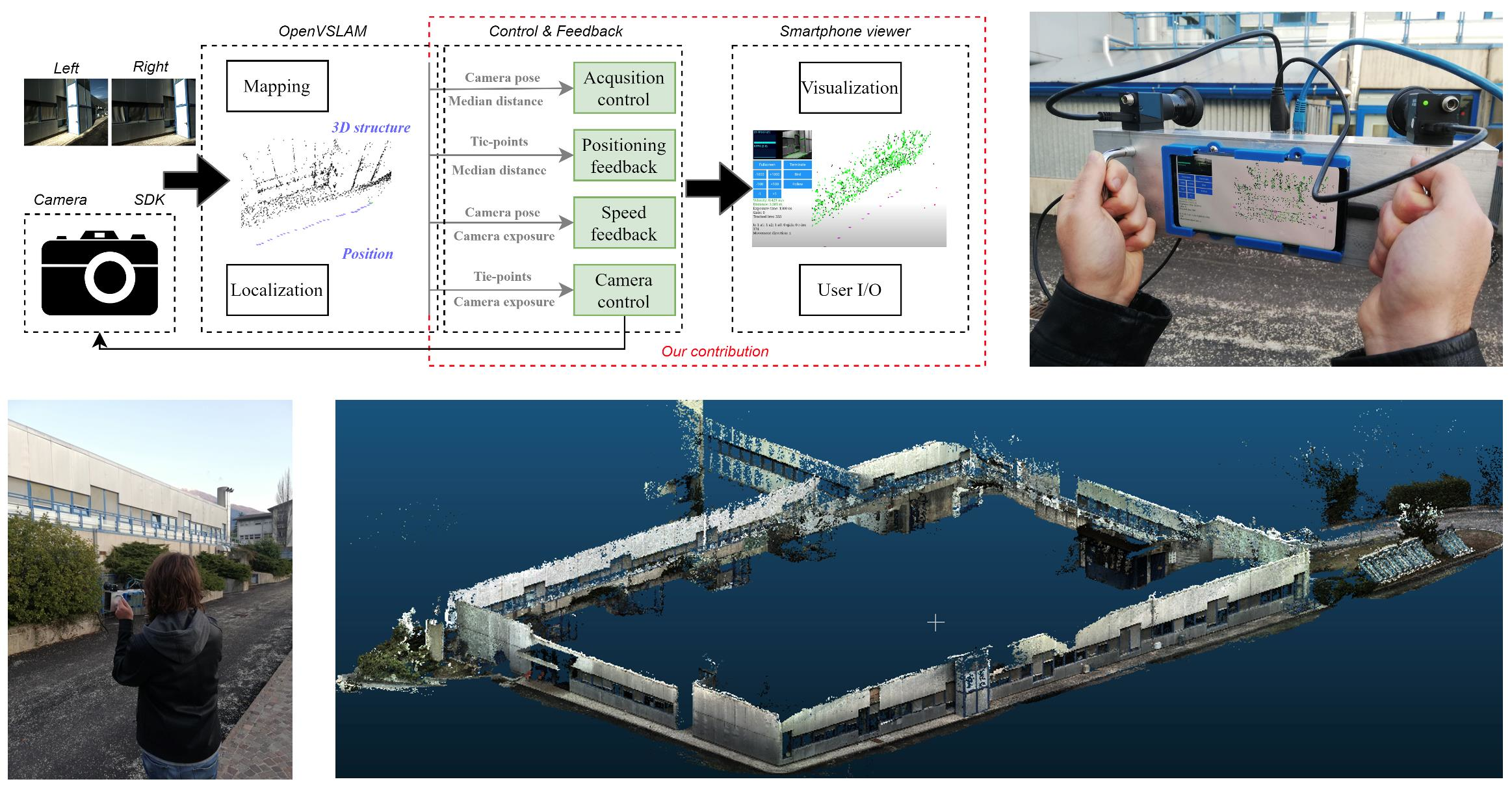
  • Realization of a flexible, low-cost and highly portable V-SLAM-based stereo vision prototype—named GuPho (Guided Photogrammetric System)—that integrates an image acquisition system with a real-time guidance system (distance from the target object, speed, overlap, automatic exposure). To the best of our knowledge, this is the first example of a portable system for photogrammetric applications with a real-time guidance control that does not use coded targets or any other external positioning system (e.g., GNSS, motion capture).
  • Modular system design based on power efficient ARM architecture: data computation and data visualization are split among two different systems (Raspberry and smartphone) and they can exploit the full computational resources available on each device.
  • An algorithm for assisted and optimized image acquisition following photogrammetric principles, with real-time positioning and speed feedback (Section 2.3.1, Section 2.3.3 and Section 2.3.3).
  • A method for automatic camera exposure control guided by the locations and depths of the stereo matched tie-points, which is robust in challenging lighting situations and prioritizes the surveyed object over background image regions (Section 2.3.4).
  • Experiments and validation on large-scale scenarios with long trajectory (more than 300 m) and accuracy analyses in 3D space by means of laser scanning ground truth data (Section 3).

2. Proposed Prototype

2.1. Hardware

A sketch of the hardware components is shown in Figure 2. The main computational unit of the system is a Raspberry Pi 4B. It is connected via USB3 to two synchronized global shutter 1 Mpixel (1280 × 1024) cameras placed in stereo configuration. They are produced by Daheng Imaging (model MER-131-210U3C) and mount 4 mm F2.0 lenses (model LCM-5MP-04MM-F2.0-1.8-ND1). The choice of this hardware was made for the high flexibility in terms of possible imaging configurations (great variety of available lenses), software and hardware synchronization, low power consumption and overall cost of the device (about 1000 Eur). The stereo baseline and angle can be adapted as needed making the system flexible to different use scenarios. The system output is displayed to the operator on a smartphone or tablet connected to the Raspberry with an Ethernet cable. This choice relieves the Raspberry from managing a GUI and leaves more resources to the V-SLAM algorithm. The very low demanding power of the ARM architectures and cameras allows the system to be powered by a simple 10,400 mAh 5 V 3.0 A power bank, which guarantees approximately two hours of continuous working activity.

2.2. Software

The proposed prototype builds upon OPEN-V-SLAM [43], which is derived from ORB-SLAM2 [42]. OPEN-V-SLAM is an indirect, graph-based V-SLAM method that uses Oriented FAST and Rotated BRIEF (ORB) [49] for data association, g2o [50] for local and global graph optimizations and DBow2 [51] for re-localization and loop detection. In addition to achieving state of the art performances in terms of accuracy, and supporting different camera models (perspective, fisheye, equirectangular) and camera configurations (monocular, stereo, RGB-D), the code of this algorithm is well modularized, making the process of integrating the guidance system much easier. Moreover, it exploits Protobuf, Socket.io, and Tree.js frameworks to easily supports the visualization of the system output inside a common web browser. This feature allows to split computation and visualization on different devices. With the aforementioned hardware (Section 2.1) and software configurations, the system can perform can work at 5 Hz using stereo pair images at half linear resolution (640 × 512 pixel).

2.3. Guidance System

A high-level overview of the system is shown in Figure 3. It is composed of three different modules (dashed boxes): (i) the camera module that manages the imaging sensors, (ii) the OPEN-V-SLAM module that embeds the localization/mapping operations and our guidance system and (iii) the viewer module that shows to the operator the system controls and output.
The realized guidance system is divided in four units:
  • Acquisition control.
  • Positioning feedback.
  • Speed feedback.
  • Camera control.
The first two units are aimed at helping the operator to acquire an ideal imaging configuration according to photogrammetric principles, thus respecting a planned acquisition distance and a specific amount of overlap between consecutive images. The last two are instead targeted at avoiding motion blur and obtaining correctly exposed images.
Let us introduce some notation before presenting more in detail the four modules of the guidance system. Let t denotes the time index of a stereo pair. At a given time t , let L t , R t be the left and right images and T t L and T t R their estimated camera poses. Finally, let d t be the estimated depth (distance to the surveyed object along the optical axis of the camera). In our approach, d t is computed as the median depth of the stereo matched tie-points between L t and R t . Thanks to the system calibration (interior and relative orientation of the cameras), all the estimated variables have a metric scale.

2.3.1. Acquisition Control

In current vision-based MMSs, it is common to acquire and store images at high frame rate (1 Hz, 2 Hz, 5 Hz, 30 Hz) and delegate at post acquisition methods [52] the task of selecting the images to use in the 3D reconstruction. This approach is extremely memory and power inefficient, especially when the images are saved in raw format.
Our prototype exploits OPEN-V-SLAM to optimize the acquisition of the images and keep their overlap constant. Let ( L s , R s ) be the last selected and stored image pair. Given a new image pair ( L t , R t ) and known their camera poses ( T t L , T t R ), the pair is considered part of the acquisition, and stored, if the baseline between the camera center of L t (resp. R t ) and the camera center of L s (resp. R s ) is bigger than a target baseline b t . b t is adapted in real-time according to the estimated distance to the object d t . More formally, b t is defined as:
b t = { w ( d t f ) ( 1 O x ) , i f   m o v e m e n t   a l o n g   c a m e r a   X   a x i s h ( d t f ) ( 1 O y ) , i f   m o v e m e n t   a l o n g   c a m e r a   Y   a x i s k , i f   m o v e m e n t   a l o n g   c a m e r a   Z   a x i s
where w and h are, respectively, the width and height of the camera sensor, f the focal length of the camera, k a constant value depending on the planned ground sample distance (GSD-Section 2.3.2), and O x , O y the target image overlaps, respectively, along the X and Y axes in decimals. The different cases ensure that the same image overlap is enforced when the movement occurs along the shortest or the longest dimension of the image sensor (Figure 4). The movement direction is detected in real-time from the largest direction cosine between the camera axes and the displacement vector between the camera centers of L t (resp. R t ) and L t 1 (resp. R t 1 ). For simplicity, the movement along the camera Z axis (forward, backward) is managed differently using a preset constant baseline k , settable by the user for the specific requirements of the acquisition. This is, in any case, an uncommon situation in standard photogrammetric acquisitions, and mostly typical of acquisitions carried out in narrow tunnels/spaces with fisheye lenses [53]. During the acquisition, the user can visualize the 3D camera poses of the selected images along with the 3D sparse reconstruction of the scenery.

2.3.2. Positioning Feedback

The ground sample distance (GSD) [54] is the leading acquisition parameter when planning a photogrammetric survey. It theoretically determines the size of the pixel in object space and, consequently, the distance between the camera and the object, measured along the optical axis. Its value is typically set based on specific application requirements.
Our system allows users to specify a target GSD range ( G S D m i n ,   G S D m a x ) and helps them to satisfy it throughout the entire image acquisition process. Usually, the GSD of an image is not uniformly distributed and depends on the 3D structure of the imaged scene. Areas lying closer to the camera will have a smaller GSD than areas lying farther away. To properly manage these situations, the system computes the GSD in multiple 2D image locations exploiting the depth of the stereo matched tie-points. The latter are then visualized over the image in the viewer, and colored based on their GSD value. Red tie-points are those having a GSD bigger than G S D m a x , green those having a GSD in the target range, and blue those having a GSD smaller than G S D m i n . This gives the user an easy-to-understand feedback about his/her actual positioning even on a limited sized display. Moreover, when the pair ( L s ,   R s ) has been deemed as part of the image acquisition by the acquisition control (Section 2.3.1), the system automatically updates the average GSD of the 3D tie-points, or landmarks in the V-SLAM terminology, matched/seen at the time s by the stereo pair ( L s ,   R s ) . In this way it is possible to finely triangulate the GSD of the acquired images over the sparse 3D point cloud of OPEN-V-SLAM. The latter can be visualized in real-time in the viewer and, exploiting the same color scheme as above, it can help the user to have a global awareness of the GSD of the acquired images, thus detecting areas where the target GSD was not achieved.

2.3.3. Speed Feedback

Motion blur can significantly worsen the quality of image acquisitions performed in motion. It occurs when the camera, or the scene objects, move significantly during the exposure phase. The exposure time, i.e., the time interval during which the camera sensor is exposed to the light, is usually adjusted, either manually or automatically, during the acquisition. This is accomplished to compensate for different lighting conditions and avoid under/over-exposed images. Consequently, also the acquisition speed should be adapted, especially when the scene is not well illuminated, and the exposure time is relatively long.
Rather than detecting motion-blur with image analysis techniques [55,56,57], our system tries to prevent it by monitoring the speed of the acquisition device and by warning the user with specific messages on the screen (e.g., using traffic light conventionally colored messages, such as “slow down” or “speed increase possible”). This approach avoids costly image analysis computations and exploits the computations already accomplished by the V-SLAM algorithm. The speed at time t , v t , is computed dividing the space travelled by the cameras, the Euclidean norm of the last two frames of the left camera centers L t and L t 1 , by the elapsed time interval. For this computation, a main assumption and simplification here is accomplished considering the imaging sensor parallel to the main object’s surface, which is typically the case in photogrammetric surveys. A speed warning is raised when:
δ t max ( G S D m i n ,   G S D m i n D )
where δ t is the space travelled by the cameras at speed v t during the current exposure time, and G S D m i n D is the GSD of the closest stereo-matched tie-point. A filtering strategy that uses the 5-th percentile of stereo matched distances is used to avoid computing the GSD on outliers. The logic behind this control is that the camera should move, during the exposure time, less than the target GSD. This ensures that the smallest details remain sharp in the images. The max function is used to avoid false warnings when the closest element in the scene is farther than the minimum GSD.

2.3.4. Camera Control for Exposure Correction

The literature of automatic exposure (AE) algorithms is quite rich, and each solution has been usually conceived to fit a particular scenario. For example, in photogrammetric acquisitions, the surveyed object should have the highest priority, even at the cost of worsening the image content of foreground and background image regions. However, distinguishing in the images the surveyed object from the background requires in general a semantic image understanding such as for example using convolutional neural networks (CNNs) [58]. Deploying CNNs on embedded systems is currently an open problem [59] for the limited resource capabilities of these systems. As a workaround, our device assumes that the stereo matched tie-points with a depth value within the target acquisition range (Section 2.3.2) are distributed, in the image, over the surveyed object. This allows us to smartly select the image regions considered by the AE algorithm, masking away the foreground and background areas that will not contribute to the computation of the exposure time. The image regions are built considering 5 × 5 pixel windows around the locations of the stereo-matched tie-points whose estimated distance lie in the target acquisition range. The optimal exposure time is then computed on the masked image using a simple histogram-based algorithm very similar to [60]. The exposure time is incremented (resp. decremented) by a fixed value Γ when the mean sample value of the brightness histogram is below (resp. above) the middle gray.

3. Experiments

The following sections present indoor and outdoor experiments realized to evaluate the camera synchronization and calibration, guidance system (positioning, speed and exposure control) and accuracy performances of the developed handheld stereo system. All the tests were performed live on the onboard ARM architecture of the system. The stereo images are downscaled to 640 × 512 pixel (half linear resolution) and rectified before being fed to OPEN-V-SLAM.

3.1. Camera Syncronization and Calibration

In the current implementation of the system, the acquisition of the stereo image pair is synchronized with software triggers, although hardware triggers are possible. We have measured a maximum synchronization error between the left and the right image of 1 ms. This has been tested recording for several minutes the display of a simple millisecond counter system using, on both cameras, a shutter speed of 0.5 ms (Figure 5a).
OPEN-V-SLAM, similar to many other V-SLAM implementations, does not perform, for efficiency reasons, self-calibration during the bundle adjustment iterations. Therefore, both the interior parameters of the cameras, and, in stereo setups, the relative orientation and baseline of the cameras, must be estimated beforehand. The calibration has been accomplished by means of bundle adjustment with self-calibration, exploiting test of photogrammetric targets with known 3D coordinates and accuracy. The calibration procedure was carried out twice: one with camera focused at 1 m for the positioning and speed feedback test (Section 3.2), and one with the cameras focused at the hyperfocal distance (1.2 m with circle of confusion of 0.0048 mm and f2.8) for the exposure (Section 3.3) and accuracy (Section 3.4) tests. In the former case we used a small 500 × 1000 mm test field composed of several resolution wedges, Siemens stars, color checkboards and circular targets placed at different heights (Figure 5b). In the latter case we used a bigger test field (Figure 5c) with 82 circular targets. In both cases, the test fields were imaged from many positions (respectively, 116 and 62 stereo pairs) and orientations (portrait, landscape) to ensure optimal intersection geometry and reduce parameter correlations. In both scenarios, some randomly generated patterns were added to help the orientation of the cameras within the bundle adjustment approach. Table 2 reports the estimated exterior camera parameters with their standard deviations.
Finally, to enable a more accurate feedback on the GSD (Section 3.2), the actual modulation transfer function (MTF) of the lens was measured using an ad-hoc test chart [61]. The chart includes photogrammetric targets that allow the relative pose of the camera to be determined with respect to the chart plane and, consequently, a better estimation of the actual GSD as well as other optical characteristics such as the depth of field. The test chart uses slant-edges according to the ISO 12233 standard. Moreover, it includes resolution wedges along the diagonals with metric scale that allow a direct visual estimation of the limiting resolution of the lens. In our experiment we compared the expected nominal GSD at the measured distance from the chart against the worst of radially and tangentially resolved patterns along the diagonals of the chart as shown in Figure 6. We estimated a ratio of about 2 considering both left and right cameras that was then used in the implemented system for a more accurate positioning feedback that is based on actual spatial resolution values attainable by our low-cost MMS.

3.2. Positioning and Speed Feedback Test

In this experiment the system positioning (Section 2.3.2) and speed (Section 2.3.3) feedback are evaluated in a controlled scenario. The experiment is structured as follow: (i) set a target GSD range of 1–2 mm; (ii) use the small test field (Figure 5b) as target object and start the image acquisition outside of the target GSD range; (iii) move closer to the object until the system says that we are in the target acquisition range; (iv) start different strips over the test field at constant distance alternating strips predicted in the speed range with strips predicted out of the speed range.
Figure 7a shows the system interface at the beginning of the test. On the top left corner there is the live stream of the left camera with the GSD-colored tie-points. Below, under the control buttons, are reported the speed of the device, the median distance to the object, the exposure and gain values of the cameras and the number of 3D tie-points matched by the image. On the right of the interface there is the 3D viewer in which are displayed the GSD-colored point cloud, the current system position (green pyramid) and the 3D positions of the acquired images (pink pyramids). The distance feedback is given at multiple levels: in the tie-point of the live image, in the median distance panel and in the 3D point cloud. All these indicators are red since we are out of the target range. Figure 7b confirms the correct feedback of the system. The thickest lines of the Siemens stars are 2.5 mm thick but they are not clearly visible. Figure 7c depicts the interface upon reaching, according to the system, the target acquisition range. All the indicators (tie-points, current distance and 3D point cloud) are green. Figure 7d confirms again the system prediction and details with 2 mm resolution can be clearly seen.
Figure 7e,f show a close view of the resolution chart in the middle of the test field during the horizontal strips over the object. The former images are taken from strips predicted in speed range, while the latter ones from strips predicted out of range. From these images it is very clear to see how, in the second case, motion blur occurred along the movement direction and evidently reduced the visible details. Despite being the image taken from a distance where theoretically it should be possible to distinguish details at 2 mm, motion blur has made even details at 2.5 hardly visible. On the other hand, when we respected the speed suggested by the system, the images remained sharp satisfying the target acquisition GSD of 2 mm.

3.3. Camera Control Test

This section reports how a camera automatic exposure (AE-Section 2.3.4) can be boosted by the V-SLAM algorithm in challenging lighting conditions. A typical situation is when the target object is imaged against a brighter or darker background. Our prototype was used to acquire two consecutive datasets of a building in situations of sky backlight. The two datasets, acquired with the same movements and trajectories, differ a few minutes between each other, so the illumination practically remained the same. The first dataset is processed using the camera auto exposure algorithm, whereas the second sequence uses the proposed masking procedure. A visual comparison of the acquired images in the first (Figure 8a) and second dataset (Figure 8b) clearly highlights the advantages brought by the proposed masking procedure to support the auto exposure in giving more importance to objects having a specific distance. Having set, for the acquired datasets, a target GSD range between 0.002 and 0.02 m, the masked images have been built in the neighborhoods of the tie-points with depth values between 0.83 and 8.3 m. Figure 8c plots the exposure time of the cameras in the two tests, where it is possible to notice, after the tenth frame, the different behavior of the AE algorithm. Figure 8d shows one of the test images with the extracted tie-points: it can be observed how they are properly distributed on the surveyed object. On the other hand, when the exposure was adjusted on the full image, it was significantly influenced by the sky brightness and underexposed the building.

3.4. Accuracy Test

A large-scale surveying scenario is used to evaluate the image selection procedure and the potential accuracy of the proposed V-SLAM-based device. The surveyed object is a FBK’s building, which spans approximately 40 × 60 m (Figure 9a). The acquisition device was handheld by an operator who surveyed the object by keeping the camera sensors mostly parallel to the building facades. To collect 3D ground truth data, the building was scanned with a Leica HDS7000 (angular accuracy of 125 μrad, range noise 0.4 mm RMS at 10 m) from 21 stations along its perimeter at an approximate distance of 10 m. All the scans were manually cleaned from the vegetation and co-registered (Figure 9b) with a global iterative closest point (ICP) algorithm implemented in MeshLab [62]. The final median RMS of the residuals from the alignment transformation was about 4 mm.
The image acquisition was performed by setting the device to acquire images in raw format with 80% overlap and a GSD range between 3 and 30 mm. The acquisition started and ended from the same positions and it lasted roughly 18 min, following device feedback on distance-to-object and speed. The overall trajectory was estimated, after a successful loop closure, about 315 m long. Along the trajectory, the acquisition control selected and saved 271 image pairs (white dots in Figure 10a). For a comparison, the common acquisition strategy of taking images at 1Hz would have acquired approximately 1080 images. The derived V-SLAM-based point cloud is color-coded with the average GSD of the selected images. The acquisition frequency was adapted to the distance to the structure, hence the irregular distance among the image pairs. Some areas of the building, such as 1 and 2 in Figure 10a, were not acquired at the target GSD due to physical limitations to reach closer positions while walking. On the other hand, a van parked in the middle of the street (area 3 in Figure 10a) forced to change the planned trajectory. This unexpected event was automatically managed by the developed algorithm that adapted the baseline in realtime to consider the shorter distance from the building.
The acquired stereo pairs were then processed offline to obtain the dense point cloud of the structure, following two approaches:
  • Directly using the camera poses estimated by our system, without further refining.
  • Re-estimating the camera poses with photogrammetric software, fixing the stereo baseline between corresponding pairs to impose the scale.
The two dense points clouds were then aligned with the laser ground truth using five selected and distributed areas (Figure 10b), achieving a final alignment error of 0.02 m (case 1.) and 0.019 m (case 2.). Agisoft Metashape was used to orient the images (case 2.) and perform the dense reconstruction (cases 1. and 2.). Finally, we computed a cloud to mesh distance between the two dense point clouds and the laser ground truth. In both cases, the errors range from a few centimeters in the south and east part of the building, to some 20 cm in the north and west ones (Figure 10c and Figure 11). In case 1., the distribution of the signed distances has a mean of 0.003 m and a standard deviation of 0.070 m (Figure 12a), with 95% of the differences bounded in the interval [−0.159, 0.166] m. The case 2. returned a slightly better error distribution (Figure 12b), with a mean value of −0.009 m, a standard deviation of 0.054 m and 95% of the differences falling in the interval [−0.144, 0.114] m. In addition to reporting the global error distribution of the building, which is significantly related to the outcome of the ICP algorithm, the local accuracy of the derived dense point cloud is also estimated using the LME (length measurement error) and RLME (relative length measurement error) [63] between seven segments (Figure 13), manually selected both on the dense point cloud obtained from the V-SLAM poses and the ground truth. The results are reported in Table 3.

4. Discussion

The presented experiments showed the main advantages brought by the proposed device. Tests to validate positioning and speed feedback (Section 3.2) have shown how the system enables a precise and easy-to-understand GSD guidance. The GSD is displayed for the current position of the device but also on the final sparse point cloud. The system also detects situations of motion blur which helps an user to prevent them. Within the camera control test (Section 3.3), exploiting the tight integration with the hardware, we took advantage of the known depth of the stereo tie-points to optimize the camera auto exposure, guiding its attention to areas that matter for the acquisition. Finally, the accuracy test (Section 3.4) showed how an image acquisition properly optimized with the scene geometry avoids over or under selections (common in time-based acquisitions) and allows to achieve satisfactory 3D results in a big and challenging scenario (Figure 10c and Figure 11). The obtained error of a few centimeters, and a RLME error around 0.5%, against the laser scanning ground truth, highlights both the quality of the image acquisition and the accuracy level reached by the developed device. The achieved results are truly inspiring if we consider the important size of the trajectory (more than 300 m), the not always collaborative surface of the building (windows, glasses and panels with poor texture-Figure 9b) and the real-time estimation of the camera poses using a simple Raspberry Pi 4. Some parts of the building, especially in the highest parts, present holes and are less accurate, but for those areas we would have required a UAV to properly record the structure with more redundancy and stronger camera network geometry. Obviously, the V-SLAM approach is meant for real-time applications therefore, considering the dimensions of the outdoor case study, we could consider satisfactory the achieved accuracy results.

5. Conclusions and Future Works

The paper presented the GuPho (Guided Photogrammetric System) prototype, a handheld, low-cost, low-powered synchronized stereo vision system that combines Visual SLAM with an optimized image acquisition and guidance system. This solution can work, theoretically, in any environment without assuming GNSS coverage or pre-calibration procedures. The combined knowledge of the system’s position and the generated 3D structure of the surveyed scene have been used to design a simple but effective real-time guidance system aimed at optimizing and making image acquisitions less error-prone. The experiments showed the effectiveness of this system to enable GSD-based guidance, motion blur prevention, robust camera exposure control and an optimized image acquisition control. The accuracy of the system has been tested in a real and challenging scenario showing an error ranging from few centimeters to some twenty centimeters in the areas not properly reached during the acquisitions. These results are even more interesting if we consider that they have been achieved with a low-cost device (ca. 1000 EUR), walking at ca 30 cm/sec, processing the image pairs in real-time at 5Hz with a simple Raspberry Pi 4. Moreover, the automatic exposure adjustment, GSD and speed control proved to be very efficient and capable of adapting to unexpected environmental situations. Finally, time-constrained applications could take advantage of the already oriented images, thanks to the V-SLAM algorithm, to speed up further processing such as the estimation of dense 3D point clouds. The built map can be stored and reutilized for successive revisiting and monitoring surveys, making the device a precise and low-cost local positioning system. Once that the survey in the field is completed, full resolution photogrammetric 3D reconstructions could be carried out on more powerful resources, such as workstations or Cloud/Edge computing, with the additional advantage of speeding up the image orientation task by reusing the approximations computed by the V-SLAM algorithm. Thanks to the system modular design, the application domain of the proposed solution could be easily extended to other scenarios, e.g., structure monitoring, forestry mapping, augmented reality or supporting rescue operations in case of disasters, facilitated also by the system easy portability, relatively low-cost and competitive accuracy.
As future works, in addition to carrying out evaluation tests in a broader range of case studies covering outdoor, indoor and potentially underwater scenarios, we will add the possibility to trigger a third high resolution camera according to the image selection criteria that will consider the calibration parameters of the third camera. We will also improve the image selection by also considering the camera rotations and by detecting already acquired areas. We are also investigating how to improve, possibly taking advantage of edge computing (5G), the real-time quality feedback of the acquisition, either with denser point clouds or with augmented reality. Finally, we are very keen to explore the applicability of deep learning to make the system more aware of the content of the images, potentially boosting the real-time V-SLAM estimation, the control of the cameras (exposure and white-balance) and the guidance system. At the end, we will investigate the use of Nvidia Jetson devices, or possibly the edge computing (5G), to allow the system to take advantage of state-of-the-art image classification/segmentation/enhancement methods offered by deep learning.

Author Contributions

The article presents a research contribution that involved authors in equal measure. Conceptualization, A.T., F.M. and F.R.; methodology, A.T. and F.M.; investigation, A.T., F.M. and R.B.; software, A.T., F.M. and R.B.; validation, A.T. and F.M.; resources, A.T.; data curation, A.T.; writing–original draft preparation, A.T.; writing–review and editing, A.T., F.M., R.B. and F.R.; supervision, F.M. and F.R.; project administration, F.R.; funding acquisition, F.R. All authors have read and agreed to the published version of the manuscript.

Funding

This work is partly supported by EIT RawMaterials GmbH under Framework Partnership Agreement No. 19018 (AMICOS. Autonomous Monitoring and Control System for Mining Plants).

Institutional Review Board Statement

Not applicable.

Informed Consent Statement

Not applicable.

Data Availability Statement

Not applicable.

Conflicts of Interest

The authors declare no conflict of interest.

References

  1. Riveiro, B.; Lindenbergh, R. (Eds.) Laser Scanning: An Emerging Technology in Structural Engineering, 1st ed.; CRC Press: Boca Raton, FL, USA, 2019. [Google Scholar] [CrossRef]
  2. Puente, I.; González-Jorge, H.; Martínez-Sánchez, J.; Arias, P. Review of mobile mapping and surveying technologies. Measurement 2013, 46, 2127–2145. [Google Scholar] [CrossRef]
  3. Toschi, I.; Rodríguez-Gonzálvez, P.; Remondino, F.; Minto, S.; Orlandini, S.; Fuller, A. Accuracy evaluation of a mobile mapping system with advanced statistical methods. Int. Arch. Photogramm. Remote Sens. Spat. Inf. Sci. 2015, 40, 245. [Google Scholar] [CrossRef] [Green Version]
  4. Nocerino, E.; Rodríguez-Gonzálvez, P.; Menna, F. Introduction to mobile mapping with portable systems. In Laser Scanning; CRC Press: Boca Raton, FL, USA, 2019; pp. 37–52. [Google Scholar]
  5. Hassan, T.; Ellum, C.; Nassar, S.; Wang, C.; El-Sheimy, N. Photogrammetry for Mobile Mapping. GPS World 2007, 18, 44–48. [Google Scholar]
  6. Burkhard, J.; Cavegn, S.; Barmettler, A.; Nebiker, S. Stereovision mobile mapping: System design and performance evaluation. Int. Arch. Photogramm. Remote Sens. Spat. Inf. Sci. 2012, 5, 453–458. [Google Scholar] [CrossRef] [Green Version]
  7. Holdener, D.; Nebiker, S.; Blaser, S. Design and Implementation of a Novel Portable 360 Stereo Camera System with Low-Cost Action Cameras. Int. Arch. Photogramm. Remote Sens. Spat. Inf. Sci. 2017, 42, 105. [Google Scholar] [CrossRef] [Green Version]
  8. Blaser, S.; Nebiker, S.; Cavegn, S. System design, calibration and performance analysis of a novel 360 stereo panoramic mobile mapping system. ISPRS Ann. Photogramm. Remote Sens. Spat. Inf. Sci. 2017, 4, 207. [Google Scholar] [CrossRef] [Green Version]
  9. Ortiz-Coder, P.; Sánchez-Ríos, A. An Integrated Solution for 3D Heritage Modeling Based on Videogrammetry and V-SLAM Technology. Remote Sens. 2020, 12, 1529. [Google Scholar] [CrossRef]
  10. Masiero, A.; Fissore, F.; Guarnieri, A.; Pirotti, F.; Visintini, D.; Vettore, A. Performance Evaluation of Two Indoor Mapping Systems: Low-Cost UWB-Aided Photogrammetry and Backpack Laser Scanning. Appl. Sci. 2018, 8, 416. [Google Scholar] [CrossRef] [Green Version]
  11. Al-Hamad, A.; Elsheimy, N. Smartphones Based Mobile Mapping Systems. ISPRS Int. Arch. Photogramm. Remote Sens. Spat. Inf. Sci. 2014, 40, 29–34. [Google Scholar] [CrossRef] [Green Version]
  12. Nocerino, E.; Poiesi, F.; Locher, A.; Tefera, Y.T.; Remondino, F.; Chippendale, P.; Van Gool, L. 3D Reconstruction with a Collaborative Approach Based on Smartphones and a Cloud-Based Server. ISPRS Int. Arch. Photogramm. Remote Sens. Spat. Inf. Sci. 2017, 42, 187–194. [Google Scholar] [CrossRef] [Green Version]
  13. Fraser, C.S. Network design considerations for non-topographic photogrammetry. Photogramm. Eng. Remote Sens. 1984, 50, 1115–1126. [Google Scholar]
  14. Nocerino, E.; Menna, F.; Remondino, F.; Saleri, R. Accuracy and block deformation analysis in automatic UAV and terrestrial photogrammetry-Lesson learnt. ISPRS Ann. Photogramm. Remote Sens. Spat. Inf. Sci. 2013, 2, W1. [Google Scholar] [CrossRef] [Green Version]
  15. Nocerino, E.; Menna, F.; Remondino, F. Accuracy of typical photogrammetric networks in cultural heritage 3D modeling projects. Int. Arch. Photogramm. Remote Sens. Spat. Inf. Sci. 2014, 45, 465–472. [Google Scholar] [CrossRef] [Green Version]
  16. Remondino, F.; Nocerino, E.; Toschi, I.; Menna, F. A Critical Review of Automated Photogrammetricprocessing of Large Datasets. ISPRS Int. Arch. Photogramm. Remote Sens. Spat. Inf. Sci. 2017, 42, 591–599. [Google Scholar] [CrossRef] [Green Version]
  17. Sieberth, T.; Wackrow, R.; Chandler, J.H. Motion blur disturbs—The influence of motion-blurred images in photogrammetry. Photogramm. Rec. 2014, 29, 434–453. [Google Scholar] [CrossRef]
  18. Iglhaut, J.; Cabo, C.; Puliti, S.; Piermattei, L.; O’Connor, J.; Rosette, J. Structure from Motion Photogrammetry in Forestry: A Review. Curr. For. Rep. 2019, 5, 155–168. [Google Scholar] [CrossRef] [Green Version]
  19. Ballabeni, A.; Apollonio, F.I.; Gaiani, M.; Remondino, F. Advances in Image Pre-processing to Improve Automated 3D Reconstruction. Int. Arch. Photogramm. Remote Sens. Spat. Inf. Sci. 2015, 8, 178. [Google Scholar] [CrossRef] [Green Version]
  20. Lecca, M.; Torresani, A.; Remondino, F. Comprehensive evaluation of image enhancement for unsupervised image description and matching. IET Image Process. 2020, 14, 4329–4339. [Google Scholar] [CrossRef]
  21. Kedzierski, M.; Wierzbicki, D. Radiometric quality assessment of images acquired by UAV’s in various lighting and weather conditions. Measurement 2015, 76, 156–169. [Google Scholar] [CrossRef]
  22. Gerke, M.; Przybilla, H.-J. Accuracy analysis of photogrammetric UAV image blocks: Influence of onboard RTK-GNSS and cross flight patterns. Photogramm. Fernerkund. Geoinf. PFG 2016, 1, 17–30. [Google Scholar] [CrossRef] [Green Version]
  23. Štroner, M.; Urban, R.; Reindl, T.; Seidl, J.; Brouček, J. Evaluation of the Georeferencing Accuracy of a Photogrammetric Model Using a Quadrocopter with Onboard GNSS RTK. Sensors 2020, 20, 2318. [Google Scholar] [CrossRef] [PubMed] [Green Version]
  24. Nex, F.; Duarte, D.; Steenbeek, A.; Kerle, N. Towards real-time building damage mapping with low-cost UAV solutions. Remote Sens. 2019, 11, 287. [Google Scholar] [CrossRef] [Green Version]
  25. Sahinoglu, Z. Ultra-Wideband Positioning Systems; Cambridge University Press: Cambridge, UK, 2008. [Google Scholar]
  26. Shim, I.; Lee, J.-Y.; Kweon, I.S. Auto-adjusting camera exposure for outdoor robotics using gradient information. In Proceedings of the 2014 IEEE/RSJ International Conference on Intelligent Robots and Systems, Chicago, IL, USA, 14–18 September 2014; pp. 1011–1017. [Google Scholar] [CrossRef]
  27. Zhang, Z.; Forster, C.; Scaramuzza, D. Active exposure control for robust visual odometry in HDR environments. In Proceedings of the 2017 IEEE International Conference on Robotics and Automation (ICRA), Singapore, 29 May–3 June 2017; pp. 3894–3901. [Google Scholar] [CrossRef] [Green Version]
  28. Taketomi, T.; Uchiyama, H.; Ikeda, S. Visual SLAM algorithms: A survey from 2010 to 2016. IPSJ Trans. Comput. Vis. Appl. 2017, 9, 16. [Google Scholar] [CrossRef]
  29. Younes, G.; Asmar, D.; Shammas, E.; Zelek, J. Keyframe-based monocular SLAM: Design, survey, and future directions. Robot. Auton. Syst. 2017, 98, 67–88. [Google Scholar] [CrossRef] [Green Version]
  30. Cadena, C.; Carlone, L.; Carrillo, H.; Latif, Y.; Scaramuzza, D.; Neira, J.; Reid, I.; Leonard, J.J. Past, Present, and Future of Simultaneous Localization and Mapping: Towards the Robust-Perception Age. IEEE Trans. Robot. 2016, 32, 1309–1332. [Google Scholar] [CrossRef] [Green Version]
  31. Sualeh, M.; Kim, G.-W. Simultaneous Localization and Mapping in the Epoch of Semantics: A Survey. Int. J. Control Autom. Syst. 2019, 17, 729–742. [Google Scholar] [CrossRef]
  32. Chen, S.; Li, Y.; Kwok, N.M. Active vision in robotic systems: A survey of recent developments. Int. J. Robot. Res. 2011, 30, 1343–1377. [Google Scholar] [CrossRef]
  33. Sünderhauf, N.; Brock, O.; Scheirer, W.; Hadsell, R.; Fox, D.; Leitner, J.; Upcroft, B.; Abbeel, P.; Burgard, W.; Milford, M.; et al. The Limits and Potentials of Deep Learning for Robotics. Int. J. Robot. Res. 2018, 37, 405–420. [Google Scholar] [CrossRef] [Green Version]
  34. Karam, S.; Vosselman, G.; Peter, M.; Hosseinyalamdary, S.; Lehtola, V. Design, Calibration, and Evaluation of a Backpack Indoor Mobile Mapping System. Remote Sens. 2019, 11, 905. [Google Scholar] [CrossRef] [Green Version]
  35. Lauterbach, H.A.; Borrmann, D.; Heß, R.; Eck, D.; Schilling, K.; Nüchter, A. Evaluation of a Backpack-Mounted 3D Mobile Scanning System. Remote Sens. 2015, 7, 13753–13781. [Google Scholar] [CrossRef] [Green Version]
  36. Kalisperakis, I.; Mandilaras, T.; El Saer, A.; Stamatopoulou, P.; Stentoumis, C.; Bourou, S.; Grammatikopoulos, L. A Modular Mobile Mapping Platform for Complex Indoor and Outdoor Environments. ISPRS Int. Arch. Photogramm. Remote Sens. Spat. Inf. Sci. 2020, 43, 243–250. [Google Scholar] [CrossRef]
  37. Davison, A.J.; Reid, I.; Molton, N.D.; Stasse, O. MonoSLAM: Real-Time Single Camera SLAM. IEEE Trans. Pattern Anal. Mach. Intell. 2007, 29, 1052–1067. [Google Scholar] [CrossRef] [PubMed] [Green Version]
  38. Klein, G.; Murray, D. Parallel Tracking and Mapping on a camera phone. In Proceedings of the 2009 8th IEEE International Symposium on Mixed and Augmented Reality, Orlando, FL, USA, 19–22 October 2009; pp. 83–86. [Google Scholar] [CrossRef]
  39. Newcombe, R.A.; Lovegrove, S.J.; Davison, A.J. DTAM: Dense tracking and mapping in real-time. In Proceedings of the 2011 International Conference on Computer Vision, Barcelona, Spain, 6–13 November 2011; pp. 2320–2327. [Google Scholar] [CrossRef] [Green Version]
  40. Engel, J.; Schöps, T.; Cremers, D. LSD-SLAM: Large-Scale Direct Monocular SLAM. In Computer Vision—ECCV 2014; Fleet, D., Pajdla, T., Schiele, B., Tuytelaars, T., Eds.; Springer: Cham, Switzerland, 2014; Volume 8690, pp. 834–849. [Google Scholar] [CrossRef] [Green Version]
  41. Mur-Artal, R.; Montiel, J.M.M.; Tardos, J.D. ORB-SLAM: A Versatile and Accurate Monocular SLAM System. IEEE Trans. Robot. 2015, 31, 1147–1163. [Google Scholar] [CrossRef] [Green Version]
  42. Mur-Artal, R.; Tardos, J.D. ORB-SLAM2: An Open-Source SLAM System for Monocular, Stereo and RGB-D Cameras. IEEE Trans. Robot. 2017, 33, 1255–1262. [Google Scholar] [CrossRef] [Green Version]
  43. Sumikura, S.; Shibuya, M.; Sakurada, K. OpenVSLAM: A Versatile Visual SLAM Framework. In Proceedings of the 27th ACM International Conference on Multimedia, Nice, France, 21–25 October 2019; ACM Press: New York, NY, USA; pp. 2292–2295. [Google Scholar] [CrossRef] [Green Version]
  44. Campos, C.; Elvira, R.; Rodríguez, J.J.G.; Montiel, J.M.M.; Tardós, J.D. ORB-SLAM3: An Accurate Open-Source Library for Visual, Visual-Inertial and Multi-Map SLAM. ArXiv200711898 Cs. Available online: http://arxiv.org/abs/2007.11898 (accessed on 12 March 2021).
  45. Snavely, N.; Seitz, S.M.; Szeliski, R. Photo tourism: Exploring photo collections in 3D. In ACM Siggraph 2006 Papers; ACM Press: New York, NY, USA, 2006; pp. 835–846. [Google Scholar]
  46. Schonberger, J.L.; Frahm, J.-M. Structure-from-motion revisited. In Proceedings of the IEEE Conference on Computer Vision and Pattern Recognition, Las Vegas, NV, USA, 27–30 June 2016; pp. 4104–4113. [Google Scholar]
  47. Trajković, M.; Hedley, M. Fast corner detection. Image Vis. Comput. 1998, 16, 75–87. [Google Scholar] [CrossRef]
  48. Calonder, M.; Lepetit, V.; Ozuysal, M.; Trzcinski, T.; Strecha, C.; Fua, P. BRIEF: Computing a Local Binary Descriptor Very Fast. IEEE Trans. Pattern Anal. Mach. Intell. 2012, 34, 1281–1298. [Google Scholar] [CrossRef] [Green Version]
  49. Rublee, E.; Rabaud, V.; Konolige, K.; Bradski, G. ORB: An efficient alternative to SIFT or SURF. In Proceedings of the 2011 International Conference on Computer Vision, Barcellona, Spain, 6–13 November 2011; pp. 2564–2571. [Google Scholar]
  50. Kummerle, R.; Grisetti, G.; Strasdat, H.; Konolige, K.; Burgard, W. G2O: A general framework for graph optimization. In Proceedings of the 2011 IEEE International Conference on Robotics and Automation, Shanghai, China, 9–13 May 2011; pp. 3607–3613. [Google Scholar] [CrossRef]
  51. Galvez-López, D.; Tardos, J.D. Bags of Binary Words for Fast Place Recognition in Image Sequences. IEEE Trans. Robot. 2012, 28, 1188–1197. [Google Scholar] [CrossRef]
  52. Torresani, A.; Remondino, F. Videogrammetry vs Photogrammetry for heritage 3D reconstruction. ISPRS Int. Arch. Photogramm. Remote Sens. Spat. Inf. Sci. 2019, XLII-2/W15, 1157–1162. Available online: http://hdl.handle.net/11582/319626 (accessed on 1 June 2021).
  53. Perfetti, L.; Polari, C.; Fassi, F.; Troisi, S.; Baiocchi, V.; del Pizzo, S.; Giannone, F.; Barazzetti, L.; Previtali, M.; Roncoroni, F. Fisheye Photogrammetry to Survey Narrow Spaces in Architecture and a Hypogea Environment. In Latest Developments in Reality-Based 3D Surveying Model; MDPI: Basel, Switzeralnd, 2018; pp. 3–28. [Google Scholar]
  54. Luhmann, T.; Robson, S.; Kyle, S.; Boehm, J. Close-Range Photogrammetry and 3D Imaging; Walter de Gruyter: Berlin, Germany, 2013. [Google Scholar]
  55. Tong, H.; Li, M.; Zhang, H.; Zhang, C. Blur detection for digital images using wavelet transform. In Proceedings of the 2004 IEEE International Conference on Multimedia and Expo (ICME) (IEEE Cat. No.04TH8763); IEEE: Toulouse, France, 2004; Volume 1, pp. 17–20. [Google Scholar] [CrossRef] [Green Version]
  56. Ji, H.; Liu, C. Motion blur identification from image gradients. In Proceedings of the 2008 IEEE Conference on Computer Vision and Pattern Recognition, Anchorage, AK, USA, 23–28 June 2008; pp. 1–8. [Google Scholar] [CrossRef]
  57. Pertuz, S.; Puig, D.; Garcia, M.A. Analysis of focus measure operators for shape-from-focus. Pattern Recognit. 2013, 46, 1415–1432. [Google Scholar] [CrossRef]
  58. Krizhevsky, A.; Sutskever, I.; Hinton, G.E. ImageNet classification with deep convolutional neural networks. Commun. ACM 2012, 60, 84–90. [Google Scholar] [CrossRef]
  59. Hinton, G.; Vinyals, O.; Dean, J. Distilling the Knowledge in a Neural Network. arXiv 2015, arXiv:1503.02531. [Google Scholar]
  60. Nourani-Vatani, N.; Roberts, J. Automatic camera exposure control. In Proceedings of the Australasian Conference on Robotics and Automation 2007; Dunbabin, M., Srinivasan, M., Eds.; Australian Robotics and Automation Association Inc.: Sydney, Australia, 2007; pp. 1–6. [Google Scholar]
  61. Menna, F.; Nocerino, E. Optical aberrations in underwater photogrammetry with flat and hemispherical dome ports. In Videometrics, Range Imaging, and Applications XIV; International Society for Optics and Photonics: Bellingham, WA, USA, 2017; Volume 10332, p. 1033205. [Google Scholar] [CrossRef]
  62. Cignoni, P.; Callieri, M.; Corsini, M.; Dellepiane, M.; Ganovelli, F.; Ranzuglia, G. MeshLab: An Open-Source Mesh Processing Tool. In Eurographics Italian Chapter Conference; CNR: Pisa, Italy, 2008; pp. 129–136. [Google Scholar]
  63. Nocerino, E.; Menna, F.; Remondino, F.; Toschi, I.; Rodríguez-Gonzálvez, P. Investigation of indoor and outdoor performance of two portable mobile mapping systems. SPIE Proc. In Proceedings of the Videometrics, Range Imaging, and Applications XIV, Munich, Germany, 26 June 2017; Volume 10332. [Google Scholar] [CrossRef]
Figure 1. The proposed handheld, low-cost, low-power prototype (named GuPho) based on stereo cameras and V-SLAM method for 3D mapping purposes. It includes a real-time guidance system aimed at enabling optimized and less error prone image acquisitions. It uses industrial global shutter video cameras, a Raspberry Pi 4 and a power bank for an overall weight less than 1.5 kg. When needed, a LED panel can also be mounted in order to illuminate dark environments as shown in the two images on the left.
Remotesensing 13 02351 g001
Figure 2. A sketch of the prototype. (a) Rear view: the operator can monitor the system output on a smartphone/tablet (S/T). (b) Front view: the Raspberry Pi 4B (RP4) is connected with USB3 to the cameras (L, R) and with Ethernet to the smartphone/tablet (S/T). The power bank (PB) is placed inside the body frame.
Remotesensing 13 02351 g002
Figure 3. High level overview of the proposed system, highlighting our contribution. The images acquired by the synchronized stereo cameras are used by the V-SLAM algorithm to estimate in real-time the local position of the device and a sparse 3D structure of the surveyed scene. Camera positions and 3D structure are used in real-time to optimize and guide the acquisition.
Remotesensing 13 02351 g003
Figure 4. Visualization, relative to the left camera of the stereo system, of the different cases considered by the acquisition control: movement along the camera (a) X axis and (b) Y axis. (c) The movement along the Z axis, less common in photogrammetric acquisitions, is handled with a preset constant baseline k.
Remotesensing 13 02351 g004
Figure 5. Some images of the millisecond counter: the maximum synchronization error amounts to 1 ms (a). Some calibration images showing the small (b) and big (c) test fields available in the FBK-3DOM lab.
Remotesensing 13 02351 g005
Figure 6. (a) Resolution chart [61] used to experimentally estimate the modulation transfer function of the used lenses. Examples of the expected resolution patches (using the designed test chart at the same resolution of 1280 pixel in width as for the camera used), respectively, at the center (b) and at 2/3 of the diagonal (c) against the imaged ones from one of the two cameras (d,e).
Remotesensing 13 02351 g006
Figure 7. System interface and the positioning and speed feedback test (af). See Section 3.2 for a detailed explanation.
Remotesensing 13 02351 g007
Figure 8. Some of the images acquired when the auto exposure (AE) algorithm uses the whole image (a) and the proposed masked image (b). (c) Plot of the exposure time in the two tests. (d) Visualization of the tie-points locations used by the AE algorithm in one of the images.
Remotesensing 13 02351 g008
Figure 9. The FBK’s building used for the device’s accuracy evaluation: (a) aerial view (Google Earth) and (b) laser scanning mesh model used as ground truth. The red dot is the starting/ending surveying position. (c) Some of the acquired images of the building: challenging glasses, reflections, repetitive patterns, poor texture surfaces and vegetation are clearly visible.
Remotesensing 13 02351 g009
Figure 10. (a) Top view of the estimated camera positions of the selected images (white squares) and derived GSD-color-coded point cloud. (b) Building areas used to align the derived dense point cloud with the laser scanning ground truth. (c) Dense point cloud obtained using the poses estimated by our system (Case 1.), with color-coded signed Euclidean distances [m] with respect to the ground truth.
Remotesensing 13 02351 g010
Figure 11. Dense point cloud obtained from the selected images with the standard photogrammetric pipeline (Case 2.) and color-coded signed Euclidean distances [m] with respect to the ground truth. The gaps in the lower left area correspond to zone #2 in Figure 10a.
Remotesensing 13 02351 g011
Figure 12. Histogram and distribution of the signed Euclidean distances [m] between the reference mesh and the dense point clouds obtained, respectively, with (a) the SLAM-based camera poses and (b) the standard photogrammetric pipeline.
Remotesensing 13 02351 g012
Figure 13. Segments considered in the LME and RLME analyses (Table 3).
Remotesensing 13 02351 g013
Table 1. Some representative and/or recent portable MMSs in the research (R) and commercial (C) domains (DOM.). They are categorized according to the format (FORM.) as handheld (H), smartphone (S), backpack (B), trolley (T), sensing devices, system architecture (SYST. ARCH.) and presence, in photogrammetry-based systems, of an onboard real-time guidance system (R.G.S.).
MMSFORM.SENSING DEVICESYST. ARCH.R.G.S.DOM.
Holdener et al. [7]HCameras (multi-view)ARMNoR
Ortiz-Coder et al. [9]HCameraX86/X64PartialR
Nocerino et al. [12]SCameraARMNoR
Karam et al. [34]BLaserX86/X64-R
Lauterbach et al. [35]BLaserX86/X64-R
Kalisperakis et al. [36]TLaser-cameras (multi-view)ARM-R
Vexcel Ultracam PantherBLaser-cameras (multi-view)X86/X64-C
GeoSLAM HorizonHLaser-cameraX86/X64-C
Leica Pegasus:backpackBLaser-cameras (multi-view)X86/X64-C
Kaarta Stencil 2HLaser-cameraX86/X64-C
OursHCameras (stereo)ARMYesR
Table 2. Calibration results. Exterior parameters of the right camera with respect to the left one.
First Calibration with Focus 1m—Small Test Field
B (mm) σ B (mm) ω (deg) σ ω (deg) φ (deg) σ φ (deg) κ (deg) σ κ (deg)
245.31670.1099−0.09350.0394−22.11230.0121−0.02390.0341
Second Calibration with Focus at Hyperfocal—Large Test Field
B (mm) σ B (mm) ω (deg) σ ω (deg) φ (deg) σ φ (deg) κ (deg) σ κ (deg)
244.99460.2388−0.09410.0136−22.47210.0079−0.011990.0055
Table 3. Measured lengths, LME and RLME between the selected segments (Figure 13).
PairLaser Data [m]Dense (SLAM-Based) Cloud [m]LME [m]RLME [%]
14.77664.75080.0258−0.5401
22.38432.37010.0142−0.5956
33.57953.58540.00590.1648
40.49480.49010.0047−0.9498
52.38882.34330.0455−1.9047
62.37302.38400.0110.4635
74.76474.78380.01910.4009
Median0.0142−0.5401
Publisher’s Note: MDPI stays neutral with regard to jurisdictional claims in published maps and institutional affiliations.

