Article

Sparse Nonnegative Matrix Factorization for Hyperspectral Unmixing Based on Endmember Independence and Spatial Weighted Abundance

Key Laboratory of Intelligent Perception and Image Understanding of Ministry of Education, International Research Center for Intelligent Perception and Computation, Joint International Research Laboratory of Intelligent Perception and Computation, School of Artificial Intelligence, Xidian University, Xi’an 710071, China
*
Author to whom correspondence should be addressed.
Remote Sens. 2021, 13(12), 2348; https://doi.org/10.3390/rs13122348
Submission received: 22 April 2021 / Revised: 29 May 2021 / Accepted: 29 May 2021 / Published: 16 June 2021
(This article belongs to the Special Issue Spectral Unmixing of Hyperspectral Remote Sensing Imagery)

Abstract

:
Hyperspectral image unmixing is an important task for remote sensing image processing. It aims at decomposing the mixed pixel of the image to identify a set of constituent materials called endmembers and to obtain their proportions named abundances. Recently, number of algorithms based on sparse nonnegative matrix factorization (NMF) have been widely used in hyperspectral unmixing with good performance. However, these sparse NMF algorithms only consider the correlation characteristics of abundance and usually just take the Euclidean structure of data into account, which can make the extracted endmembers become inaccurate. Therefore, with the aim of addressing this problem, we present a sparse NMF algorithm based on endmember independence and spatial weighted abundance in this paper. Firstly, it is assumed that the extracted endmembers should be independent from each other. Thus, by utilizing the autocorrelation matrix of endmembers, the constraint based on endmember independence is to be constructed in the model. In addition, two spatial weights for abundance by neighborhood pixels and correlation coefficient are proposed to make the estimated abundance smoother so as to further explore the underlying structure of hyperspectral data. The proposed algorithm not only considers the relevant characteristics of endmembers and abundances simultaneously, but also makes full use of the spatial-spectral information in the image, achieving a more desired unmixing performance. The experiment results on several data sets further verify the effectiveness of the proposed algorithm.

Graphical Abstract

1. Introduction

With the continuous improvement of science and technology, remote sensing images have been developed by leaps and bounds. Hyperspectral image (HSI), a kind of remote sensing image, has attracted the attention of many researchers due to its rich spectral information [1,2,3]. HSI contains dozens or even hundreds of continuous bands, and each pixel can be extracted to a complete spectral curve that reflects the characteristics of ground objects. Thus, it has been successfully applied to many aspects, such as agriculture, meteorology, exploration and so on. However, there is a variety of materials mixed in a pixel, i.e., the phenomenon of spectral mixing. The spectral mixing will seriously affect the subsequent processing of HSI, such as classification [4], detection [5,6], etc. Therefore, the decomposition of mixed pixels for HSI becomes more and more crucial.
Mixed pixel decomposition of HSI, referred to as hyperspectral unmixing (HU), is to decompose the mixed pixel into several materials (endmembers) and to obtain their proportions (abundances). The models for HU are mainly divided into linear mixing model (LMM) and nonlinear mixing model [7]. The LMM assumes that each photon acts on only one material with no interactions among them. It is easy to be solved and can meet the basic needs of research, which has been widely used in HU. This paper is also based on the LMM for unmixing research. The process of HU generally contains three steps: endmember number estimation, endmember extraction and abundance estimation. There are many traditional algorithms for endmember number estimation, such as hyperspectral signal identification by minimum error (Hysime) [8], virtual dimensionality (VD) [9], minimum noise fraction [10]. Based on different assumptions, the endmember extraction algorithms can be grouped into the methods based on pure pixel, minimum volume, statistics, etc. The well-known algorithms for endmember extraction contain pixel purity index (PPI) [11], N-FINDR [12], vertex component analysis (VCA) [13] and so on. Besides, two kinds of constraints for abundances exist in HU, i.e., the abundance nonnegative constraint (ANC) and the abundance sum to one constraint (ASC). The former requires that the abundance value is nonnegative, and the latter asks the sum of abundance value of each pixel to be one. Nonnegative constrained least squares algorithm and fully constrained least squares (FCLS) algorithm [14] are two unmixing methods based on LMM combined with different constraints of abundances. The algorithms of VCA and FCLS are often adopted as the initial method for endmember extraction and abundance estimation in the experiment. In addition, numerous different algorithms have been proposed, including the geometric analysis method [15], filtering method [16], deep learning [17], etc. Based on the characteristics of hyperspectral images and some prior information, researchers present a series of abundance estimation algorithms.
The sparse unmixing (SU) algorithm provides an important direction for the research. Studies have stated that as for HSI, not all endmembers of the image participate in the mixing of each pixel, but only a few [18]. Correspondingly, the abundance is sparse. In addition, due to the widely available spectral library, the SU algorithm is able to measure the situation when the pure pixels do not exist in the image [19]. Lots of classical sparse unmixing algorithms appear in view of the different priors and understandings for HSI. The commonly used norms for sparsity constraint are L1 regularization, L1/2 regularization and L2,1 regularization. The solution obtained by L1/2 regularization is sparser than that by L1 regularization [20]. The sparse unmixing by variable splitting and augmented Lagrangian (SUnSAL) [19] algorithm explores the L1 norm as the constraint for abundance based on the alternating direction method of multipliers to solve the sparse regression problem. However, it just analyzes the hyperspectral data and does not incorporate the spatial information. In order to make use of the spatial information in the image, the sparse unmixing via variable splitting augmented Lagrangian and total variation (SUnSAL-TV) algorithm adds the total variation of regularization to the model of SUnSAL algorithm [21]. Furthermore, the collaborative SUnSAL (CLSUnSAL) [22] considers the pixels in HSI sharing the same active set of atoms in the library and employs the L2,1 regularization for collaborative sparse regression. Local collaborative sparse regression unmixing algorithm imposes the collaborative sparsity among neighboring pixels, which assumes that the neighboring pixels share the same active set of endmembers [23]. The spatial discontinuity-weighted sparse unmixing [24] adopts a spatial discontinuity weight for SUnSAL to preserve the spatial details of abundance. The joint local block grouping with the noise-adjusted principal component analysis sparse method [25] utilizes the local block grouping to get spatial information and draws the representative spatial correlations obtained by the noise-adjusted principal component analysis for unmixing. Besides, with the intention to take advantage of the spatial information, spectral and spatial weighting factors are exploited by the spectral-spatial weighted sparse unmixing framework, imposing the sparsity of solution [26]. Although the SU algorithm has made some achievements, the spectra collected in the spectral library and the image show there are still many differences that raise doubts.
The nonnegative matrix factorization (NMF)-based unmixing approach is another highlighted branch for HSI, which has attracted the attentions of researchers due to its successful applications in many fields. The main task of NMF [27] is decomposing a nonnegative matrix into the product of two nonnegative matrices to reduce the dimension of high-dimensional data. Since its goal is similar to that of spectral unmixing, the NMF model has been widely employed in unmixing. However, the NMF model has an ill-conditioned problem, which tends to fall into a local optimal solution. Therefore, it is necessary to add some specific constraints of endmembers and abundances to the NMF model based on the characteristic of HU. Casalino et al. added both sparsity constraint and spatial information to a new nonnegative matrix under approximation model [28]. Scholars put forward lots of excellent NMF-based algorithms that achieve good effects for HU [29,30,31,32]. Qian et al. introduced the L1/2 sparsity NMF for HU through the L1/2 regularization raised in [20] to make the solution sparser and more accurate [18]. Miao et al. presented the minimum-volume constraint NMF (MVCNMF) by a geometric constraint of endmembers [33]. Li et al. performed three steps of HU together in the robust collaborative NMF (CoNMF) [34]. Inspired by the manifold learning, Lu et al. added the graph regularized constraint in NMF (GLNMF) to fully exploit the latent manifold structure of HSI [35]. Wang et al. divided the pixels of HSI into groups based on their correlation and used a spatial group sparsity regularization term for abundance to unmix [36]. Under the self-learning semi-supervised framework, Wang et al. integrated the prior information into NMF as the constraints of endmembers and abundances in the unmixing process [37]. Xiong et al. brought a nonconvex non-separable sparse NMF approach via a generalized minimax concave sparse regularization preserving the convexity of NMF for each variable [38].
Inspired by the advantage of NMF model, we develop a sparse NMF unmixing algorithm based on endmember independence and spatial weighted abundance for HSI (EASNMF). The purpose of the proposed algorithm is to make the extracted endmembers independent of each other and obtain smooth abundances. For the endmembers, it is considered that the more independent the endmembers are, the better they can characterize the HSI. Thus, the constraint of endmembers via autocorrelation matrix is added to the NMF model. In addition, only a subset of endmembers participates in the mixing of pixels, which leads to the sparsity of abundances. Therefore, we adopt the sparse constraint for abundances and introduce a weight in view of spatial information to make the abundances smoother. Furthermore, in order to exploit the latent manifold structure of the HSI data, manifold regularization is also employed in our model. The results on both the simulated data set and the real data set demonstrate the effectiveness of the proposed EASNMF algorithm with the flowchart shown in Figure 1. In general, the EASNMF algorithm not only puts forward the appropriate constraints based on the characteristics of endmembers and abundances, but also fully integrates the spatial-spectral information for HU.
The rest of this paper is arranged as follows. Section 2 is the related work, Section 3 introduces the proposed EASNMF algorithm in detail, followed by Section 4 of the experiment, and finally, the conclusion is in Section 5.

2. Related Work

2.1. LMM

The unmixing algorithms often rely on the establishment of the mixing models, and the LMM is an important mixing model. Let Y L × P represent the HSI observation matrix of L bands and P pixels, E L × K indicate the endmember matrix with K endmembers, A K × P mean the abundance matrix and N L × P refer to the noise matrix, thus the LMM can be formed as follows:
Y = E A + N
Two constraints of abundances including the ANC and ASC are below:
ANC :   a ij 0 , i , j
ASC :   i = 1 K a i j = 1 , j = 1 : P
where a i j is the abundance value of i-th endmember at j-th pixel of the HSI.

2.2. NMF

NMF, a powerful tool for statistical analysis, is one commonly used model for HU due to its significant advantages. The standard form of the NMF model based on the cost function of Euclidean distance is as follows:
min E , A   1 2 Y E A F 2 , s . t .   E 0 ,   A 0
where F denotes the Frobenius norm. The purpose of NMF is to seek two nonnegative matrices decomposed from the HSI data.
To optimize the function with respect to E and A in Equation (4), the updated rules of the iterative algorithm proposed in [27] are below:
E E ( Y A T ) ( E A A T )
A A ( E T Y ) ( E T E A )
where ( ) T refers to the transpose of matrix, and are the elementwise multiplication and division, called Hadamard product and Hadamard division, respectively.
However, due to the nonconvex objective function of the NMF model in Equation (4), it suffers from the problem of nonunique solution. Therefore, to reduce the feasible solution set, some constraints based on the characteristics of endmembers and abundances are introduced to the NMF model. There are various constraints to solve this problem, such as manifold constraint [39,40], sparseness constraint [41], low-rank constraint [42], smooth constraint [43] and so on. These NMF-based approaches are all named constrained NMF, with the formulation as follows:
min E , A   1 2 Y E A F 2 + λ f ( E ) + μ φ ( A ) s . t .   A 0 ,   1 K T A = 1 P T
where f ( E ) and φ ( A ) are the constraints of endmembers and abundances, and the two parameters λ and μ separately adjust the effects of the corresponding regularization term in Equation (7).

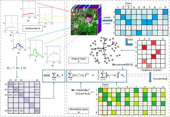
3. Sparse NMF for Hyperspectral Unmixing Based on Endmember Independence and Spatial Weighted Abundance

In this section, the proposed sparse unmixing algorithm based on endmember independence and spatial weighted abundance with manifold regularization is introduced in detail. The raised EASNMF algorithm can get the independent endmembers and the smooth abundances, which fully exploits the spatial-spectral information and the intrinsic geometrical characteristics of HSI data.

3.1. Endmember Independence Constraint

As we know, the solution space of the NMF model is very large. In addition, the endmembers are very important to unmixing research, which will affect the effect of HU. Therefore, we can utilize this characteristic of endmembers as the prior knowledge added to NMF model. This way, the accurate endmembers can be received to further improve the unmixing effect. The HSI data is formed by different endmembers with a certain proportion, and it is easy to find that the endmembers should be independent of each other. For the independence, the autocorrelation matrix can be adopted to constrain the endmembers. If the endmembers are independent from each other, their autocorrelation matrix should be a diagonal matrix. That is, the off-diagonal elements of its autocorrelation matrix should be as close to 0 as possible. Therefore, the NMF model with endmember independence constraint is as follows:
min E , A   1 2 Y E A F 2 + α ( E T E 1 E F 2 )   s . t .   A 0 ,   1 K T A = 1 P T
where α is the parameter to balance the data fidelity and endmember independence term. The second term refers to the sum of the off-diagonal elements of the autocorrelation matrix for endmembers, i.e., the difference between the sum of all the elements (the first sub-term) and the sum of the diagonal elements (the second sub-term). The purpose for the second term in Equation (8) is to make the endmembers independent of each other as much as possible; that is, the correlation between different endmembers should be as small as possible.

3.2. Abundance Sparse and Spatial Weighted Constraint

Studies have shown that most of the mixed pixels are mixtures with only a few endmembers on the scene [41]. That is to say, the mixed pixel is likely to be the superposition of only a few endmembers, not all endmembers. Thus, the corresponding abundance is sparsity, which can be considered an intrinsic property of HU. Therefore, the sparsity constraint as an effective tool has been introduced to HU. As mentioned before, the L1/2 regularizer proposed by [20] is proved to provide a sparse and accurate result. Taking the sparsity of abundance into consideration, we add the sparse constraint of abundance into the model, which is formed as follows:
min E , A   1 2 Y E A F 2 + α ( E T E 1 E F 2 ) + β A 1 2   s . t .   A 0 ,   1 K T A = 1 P T
where β is the weight parameter to adjust the effect of the last term in Equation (9), and A 1 / 2 = i , j K , P ( a i j ) 1 / 2 .
Moreover, the neighboring pixels are more likely to have similar fractional abundance values, which is considered spatial structure information. This information can be constructed as a weight matrix for abundances to make full use of. Suppose the pixel y j , whose corresponding abundance value is a j , is one neighbor of the pixel y i , and there are m neighbors for pixel y i . For each iteration of abundance, the abundance average of the neighborhood for each pixel is calculated to construct a weight matrix W = [ w 1 , w 2 , , w i ] K × P for next iteration. The element in weight matrix W is computed as follows:
w i ( k + 1 ) = 1 ( 1 m j = 1 m a j ) ( k ) + e p s y j ( y i )
where eps is a predetermined positive constant. Here the Euclidean distance is adopted to calculate the similarity of pixels in the image, and then m pixels with smallest values are chosen as the neighbors to obtain the element of weight matrix W in Equation (10). It is hoped that if the spectral signatures of pixels are similar, their abundance values should be similar. The model with the weight matrix W is expressed as below:
min E , A   1 2 Y E A F 2 + α ( E T E 1 E F 2 ) + β W A 1 2   s . t .   A 0 ,   1 K T A = 1 P T
where is the term-by-term Hadamard product.
In this part, the priors of sparseness and spatial information are integrated into the NMF model to shrink the solution space and further promote the unmixing performance. However, it just considers the sparse characteristic for unmixing and neglects the intrinsic geometrical structure of HSI. Therefore, it is necessary to further explore the potential characteristic of HSI data for unmixing.

3.3. Manifold Regularization Constraint

As is well known, HSI is a kind of high-dimensional data. Recently, researchers showed that the hyperspectral data vary smoothly along the geodesics of the data manifold and tend to lie on a low-dimensional subspace embedded in the high-dimensional data space [35]. Moreover, the manifold learning finds the representation in low-dimensional manifold space for high-dimensional space data. It can dig into the essence of data and discover its inherent laws. In Equation (11), only the sparse characteristic and the Euclidean structure of hyperspectral data are taken into account as we have posted before. Therefore, it is necessary to introduce the intrinsic manifold structure into the proposed model to render better performance of HU.
There are P pixels in HSI and each pixel can be considered a data point. Thus, the nearest neighbor graph is constructed by each pixel as its vertices and its weight matrix is denoted as W g . The weight between two pixels y i and y j is defined as follows:
w g i j = { c o r r c o e f ( y i ,   y j ) y i ( y j )   o r   y j ( y i ) 0 o t h e r w i s e
Here c o r r c o e f ( ) means the correlation coefficient and it is calculated by c o v ( y i , y j ) v a r ( y i ) v a r ( y j ) where c o v ( ) and v a r ( ) separately mean the covariance and variance. That is, if the pixel y j is a neighbor of pixel y i , the weight between these two pixels is obtained by computing their correlation coefficient. The correlation coefficient is usually used to describe the degree of correlation between two variables in statistics, whose absolute value is between 0 and 1. Generally speaking, the closer its absolute value is to 1, the greater the correlation between two variables is.
Furthermore, based on the analysis before, if two pixels y i and y j are close in the original space, their representations a i and a j in the new space should also be close [35]. For this purpose, the manifold constraint is proposed as below:
1 2 i , j = 1 P a i a j 2 w g i j = i = 1 P a i T a i d i i i , j = 1 P a i T a j w g i j = T r ( A D A T ) T r ( A W g A T ) = T r ( A L A T )
where T r ( ) indicates the trace of the matrix, d i i = j = 1 P w g i j and L = D W g . Then, incorporating the manifold regularization into the model, the finial objective function is exhibited as follows:
min E , A   1 2 Y E A F 2 + α ( E T E 1 E F 2 ) + β W A 1 2 + γ 2 T r ( A L A T )   s . t .   A 0 ,   1 K T A = 1 P T
where γ acts as the penalty parameter to control the manifold regularization term.
According the updated rule in [20], the iterative solution of Equation (14) is presented as follow.
E E ( Y A T ) ( E A A T + 2 α E I 1 2 α E )
A A ( E T Y + γ A W g ) ( E T E A + β 2 W 1 2 A 1 2 + γ A D )
where I1 is the matrix with all 1 elements. Considering the ASC, a simple and effective technique in [35,41] is employed. When updating the abundance A by Equation (16), the matrices Y and E will be replaced by Y f and E f by adding a row as the inputs to achieve the ASC, which are defined as below:
Y f = [ Y ε 1 P T ] E f = [ E ε 1 K T ]
where the parameter ε controls the influence of ASC, and in our experiment, it is set to be 15, which will be mentioned later. Then taking the ASC into consideration, the iterative criterion for abundance is as follows:
A A ( E f T Y f + γ A W g ) ( E f T E f A + β 2 W 1 2 A 1 2 + γ A D )
The whole algorithm has been described in detail. Our algorithm not only proposes the appropriate constraints based on the characteristics of endmembers and abundances simultaneously, but also makes full use of the spatial-spectral information in the image, achieving a desired unmixing performance. Algorithm 1 briefly presents the solution to Equation (14) and summarizes the aforementioned description; the values of parameters α, β and γ will be discussed in detail later.
Algorithm 1 Sparse NMF for HU Based on Endmember Independence and Spatial Weighted Abundance
1. Input: The hyperspectral image Y, the number of endmember K, the parameters α, β and γ.
2. Output: Endmember matrix E and abundance matrix A.
3. Initialize E and A by VCA-FCLS algorithm, W by Equation (10), Wg by Equation (12), and D.
4. Repeat:
5. Update E by Equation (15).
6. Augment Y and A separately to get Yf and Af.
7. Update A by Equation (18).
8. Update W by Equation (10).
9. Until stopping criterion is satisfied.

4. Experiments Results

This section mainly describes a series of experiments designed to evaluate the effectiveness of the proposed EASNMF method. We first introduce the evaluation metrics and the data sets including the simulated data set and the real data set. Then the experimental setting is explained. Finally, the results of the EASNMF algorithm and the comparisons composed of MVCNMF, L1/2-NMF, GLNMF and CoNMF on both the simulated data set and the real data set are displayed and analyzed.

4.1. Performance Evaluation Criteria

In the experiment of this paper, two widely adopted evaluation metrics are used to measure the accuracy separately for endmembers and abundances. First is the spectral angle distance (SAD), which can qualify the similarity of the extracted endmember and its real endmember by calculating their spectral angle. When the SAD value is smaller, the performance for endmember extraction is better. Besides, the SAD is not affected by spectral scale either, whose definition is as below:
S A D = arccos ( E T E ¯ E E ¯ )
where E and E ¯ are the real endmember and the extracted endmember.
The error between the abundance and its real abundance is computed by the root-mean-square error (RMSE) in the experiment, which is formed as follows:
R M S E = ( 1 P A A ¯ 2 ) 1 2
where A represents the real abundance and A ¯ denotes the estimated abundance. When the estimated abundance is close to the real abundance, the error is small corresponding to the good performance for abundance estimation.

4.2. Data Sets

There are three data sets employed in the experiment to evaluate the effectiveness of the EASNMF algorithm, which contains two simulated data sets and one real data set called Cuprite.
  • Simulated data set 1:
The first simulated data set provided by Dr. M. D. Iordache and Prof. J. M. Bioucas-Dias is generated with 100 × 100 pixels and nine spectra randomly selected from the USGS spectral library [44]. Its abundance maps are shown in Figure 2 for illustrative purposes. This data set has 224 bands and its abundance follows a Dirichlet distribution. Owing to its good spatial homogeneity, it becomes the data set widely used in HU [25,38]. Finally, the Gaussian noise with 30 dB was added.
  • Simulated data set 2:
The second data set is provided in the HyperMix tool [45] with 100 × 100 pixels and 221 bands for testing the spectral unmixing algorithms. There are nine endmembers randomly selected from the USGS library after removing certain bands for this data set. The fractional abundance maps associated with each endmember are displayed in Figure 3. Similar to the simulated data set 1, the Gaussian noise with 30 dB was included in the experiment.
  • Cuprite data set
The scene adopted in the real data experiment is named Cuprite data set, which was captured by airborne visible infra-red imaging spectrometer (AVIRIS) in 1997. Since the Cuprite data set contains rich minerals that are usually highly mixed, it is a popular data set for researchers to verify the effectiveness of the HU algorithm [23,37,41]. A sub-image with 250 × 191 pixels is selected from the scene containing 224 spectral bands ranging from 400 to 2500 nm. Figure 4 shows the real data set (left) and the reference maps (right) produced by Tricorder 3.3 software product in 1995, which maps different minerals presented in the mining district. Although it is inappropriate to compare the distribution map directly with Cuprite data set, the reference map can still be used in qualitative analysis of abundance map evaluation. Besides, its resolutions of spectral and spatial are approximately 10 nm and 20 m. The bands 1–2, 105–115, 150–170, and 223–224 affected by water vapor and atmospheric were removed remaining 188 bands. The agreement for the endmember number is not available, a frequently used and widely recognized number is twelve, including alunite, andradite, buddingtonite, dumortierite, kaolinite1, kaolinite2, montmorillonite, muscovite, nontronite, pyrope, sphene and chalcedony.

4.3. Compared Algorithms

In our experiment, four unmixing algorithms listed as follows are selected as the comparisons for the proposed EASNMF algorithm:
  • L1/2-NMF algorithm: it extends the NMF method by incorporating the L1/2 sparsity constraint, which provides a more sparser and accurate results [18].
  • GLNMF algorithm: it incorporates the manifold regularization into sparsity NMF, which can preserve the intrinsic geometrical characteristic of HSI data during the unmixing process [35].
  • MVCNMF algorithm: it adds the minimum volume constraint into the NMF model and extracts the endmember from highly mixed image data [33].
  • CoNMF algorithm: it performs all stages involved in HU process including the endmember number estimation, endmember estimation and abundance estimation [34].

4.4. Initializations and Parameter Settings

There are several important issues that need to be addressed in advance. The details of these issues are discussed below.
  • Initialization: the initialization of endmember and abundance is the first issue. In our experiment, we choose the VCA-FCLS algorithm, one basic method for endmember extraction and abundance estimation, as our initialization method to speed up the optimization. VCA algorithm [13] exploits two facts to extract the endmembers: the endmembers are the vertices of a simplex and the affine transformation of a simplex is also a simplex. FCLS algorithm, a quadratic programming technique, is developed to address the fully constrained linear mixing problems, which uses the efficient algorithm to simultaneously implement both the ASC and ANC [14].
  • Stopping criterion: it is another important issue and two stopping criteria are adopted for the optimization, i.e., error tolerance and maximum iteration number. When any stop condition is reached, the algorithm stops. When the error is successively within the limits of tolerance, a predefined value, the iteration is stopped. The error tolerance is set as 1.0 × 10⁻⁴ for a simulated data set and 1.0 × 10⁻³ for the real data set in our experiment. The times of iteration meet the maximum iteration number, the optimization ends. The maximum iteration number is set as 1.0 × 10⁶ in experiment.
  • ANC and ASC: for the abundance, its initial value obtained by VCA-FCLS algorithm is generally nonnegative. Thus, according to the update rule recorded in Equations (15) and (16), the E and A are obviously nonnegative. Besides, considering the ASC, the A adopted by Equation (18) also satisfies the constraint. Moreover, the parameter ε in Equation (17) controls the convergence rate of ASC. When its value is large, it will lead to an accurate result but with lower convergence rate. As in many papers [35,41], the parameter ε is set as 15 in the experiments for desired tradeoff.
  • Parameter setting: there are three parameters in the proposed model, i.e., α, β, γ. They separately control the independence constraint of the endmember, abundance sparse constraint, and the manifold constraint, which will be analyzed in detail in next part of the experiment.
  • Endmember number: the endmember number is one of the crucial processes in HU, which is another independent topic. In our experiment, it is considered a topic that does not have much relation to this paper and it is assumed to be known. In fact, the algorithms of HySime [8] and VD [9] could be adopted to estimate the number of endmembers. Hysime algorithm [8] is a new minimum mean square error-based approach to infer the signal subspace in hyperspectral imagery. In the experiment, we can also analyze the number of endmembers around the number estimated by Hysime algorithm via the reconstruction error.
  • Computational complexity: here, we analyze the computational complexity of the proposed EASNMF algorithm. It is noticeable that the matrix Wg is sparse and there are m nonzero elements in each row. Therefore, the floating-point addition and multiplication for AWg in Equation (16) cost mPK times. Additionally, the computing cost of A−1/2 is (PK)2. Except for these costs, the other three floating-point calculation times for each iteration are listed in Table 1.

4.5. Experiment on Simulated Data Set 1

In this section, we evaluate the proposed EASNMF method by the simulated data set 1 to investigate it precisely. The three parameters, including α, β and γ, need to be determined in advance. As mentioned earlier, the parameter α controls the endmember independence term, the parameter β adjusts the effect of abundance sparse constraint and the parameter γ is the penalty parameter for manifold regularization. Figure 5 shows the curves of these three parameters with respect to SAD and RMSE. From Figure 5a,b, it can be easily found that both of the SAD and RMSE curves are not sensitive to the parameter α. Besides, the curves of SAD and RMSE generally rise with the increasing of parameter β. Moreover, Figure 5b demonstrates that when the parameter γ is around 1, the values of SAD and RMSE are small. It corresponds to the good unmixing effect for endmember extraction and abundance estimation. Therefore, the parameters α, β and γ are separately set as 0.01, 0.001 and 1.
After determining the parameters of the proposed model, we perform our algorithm with simulated data set 1. Figure 6 shows the reference endmember curves with a red solid line and the estimated endmember curves obtained by EASNMF method with a blue dotted line. Through the observation and analysis of Figure 6, we can see that most estimated endmembers are very close to the reference, and there are some small differences between the references and estimations for endmembers 3 and 9. In general, the endmembers obtained by the proposed method are in good accordance with the referenced ones, which demonstrates the satisfactory endmember estimations provided by EANMF algorithm.
At the same time, we also exhibit the abundance maps of the proposed method and compare it with some related algorithms to illustrate its effectiveness for unmixing. The comparison algorithms include the methods of L1/2-NMF, GLNMF, MVCNMF and CoNMF. The results of the EASNMF algorithm and the comparisons are displayed in Figure 7. Due to the limited space of the paper, here the abundance maps of only three representative endmembers are exhibited, and they are endmembers 2, 6, and 9, respectively. Comparing to the real abundance maps in Figure 2, it can be observed that the abundance map obtained by the EASNMF algorithm is smoother than that of L1/2-NMF algorithm, especially in the homogeneous part for endmember 9. In addition, the result of GLNMF algorithm is satisfactory with some details missing, such as the texture of homogeneous region in Figure 7a. Since there is no constraint on abundance, the background of multiple abundance maps extracted by MVCNMF algorithm is messier than the other methods. Although the CoNMF algorithm can handle the steps of endmember number estimation, endmember extraction and abundance estimation together, it does not put forward some specific constraints, making the extracted abundance not ideal. In general, the performance of the proposed EASNMF algorithm is satisfied, which illustrates its effectiveness for HU.
Furthermore, in order to quantitatively evaluate the algorithms, we also calculate the values of SAD and RMSE by Equations (19) and (20). For the purpose of comparing, the SAD value and RMSE value of the EASNMF algorithm and comparisons are listed in Table 2. Simultaneously, the SAD value and the RMSE value for each endmember are also recorded in Table 2. Based on the values in Table 2, the results of MVCNMF and CoNMF are worse than the other comparisons, whether for the endmembers or the abundances. In addition, it can be noted that compared to the listed comparisons, the best and second-best results are mostly obtained by EASNMF algorithm. Owing to the appropriate constraints based on the endmember independence and spatial weight, the performance of the proposed method is slightly higher than the listed comparison algorithms for unmixing.

4.6. Experiment on Simulated Data Set 2

In this section, we perform the proposed method on simulated data set 2, whose results will be shown and analyzed in detail. Similarly, it needs to analyze the parameters in model before the experiment. Figure 8 presents the curves of SAD and RMSE values with different values of three parameters α, β and γ. From Figure 8, the overall values of SAD and RMSE are relatively low, demonstrating the effectiveness of endmember extraction and abundance estimation. Besides, it is not difficult to find that the parameter α has a small effect on the values of SAD and RMSE in the local interval. When parameter β is small, the corresponding SAD and RMSE values are relatively small, indicating the good performance of unmixing. With the increase of parameter γ, the values of SAD and RMSE gradually decrease, and their curves tend to be stable around γ = 1. Thus, the parameters α, β and γ are separately set as 0.1, 0.01, 1.
In our paper, the endmember number is another important issue for HU, which is assumed to be known. Here, we can also use the reconstruction error defined by Y E ¯ A ¯ 2 to analyze the endmember numbers in the experiment [34]. Figure 9 exhibits the curve of reconstruction error with respect to different endmember numbers. As the endmember number increases, the error decreases and tends to be stable. It can be seen from the curve in Figure 9, when the endmember number is 9, the error is the smallest.
In order to indicate clearly the difference between the experimental results of different methods and the references on simulated data set 2, Figure 10 displays the error maps of abundances obtained by EASNMF algorithm and comparisons. In the error maps, the closer the color is to blue, the smaller the error is. Due to the limitation of the space, we only present the error maps of abundances corresponding to three typical endmembers, i.e., endmembers 3, 5 and 9. It can be seen from Figure 10 that the result of CoNMF algorithm is the worst and there are some scattered points on the error map of L1/2-NMF algorithm. Since the MVCNMF algorithm does not have any abundance constraints in its model for unmixing, the error distributes in the whole image without any spatial structure information. Although the error maps of the GLNMF algorithm and EASNMF algorithm are somewhat similar, the overall color of the error maps obtained by EASNMF method is darker than that of GLNMF algorithm, indicating a small error in general. In addition, owing to the smoothness constraint on abundance, the error distribution of the proposed algorithm is relatively smoother than the comparisons, especially for endmembers 3 and 9. Due to the complexity of the data set scene, the advantage of the proposed algorithm is not obvious which is the limitation for the proposed algorithm. In general, the proposed algorithm is effective for unmixing.
Furthermore, Table 3 records the SAD value and RMSE value of the EASNMF algorithm and comparisons, including the average value and the value corresponding to each endmember. Due to the fact that the spatial distribution of this data set is trivial, the advantage of spatial constraints in unmixing model is not obvious. That is the reason that for some endmembers, the performance of the L1/2-NMF is better than the other algorithms. Through comparison and analysis, we can find that the algorithms of GLNMF and MVCNMF is similar and the performance of CoNMF algorithm is the worst. Since we utilize the characteristic of endmembers and abundances and exploit the latent structure of data, the proposed method makes full used of the spatial-spectral information in the image. On the whole, in terms of the average value of SAD and RMSE values, the EASNMF algorithm obtains the smallest values. Although the improvement is not obvious to average values, it still demonstrates its effectiveness for HU.

4.7. Experiment on Cuprite Data Set

We turn our attention to the real data set. The real data set adopted in the experiment is Cuprite data set, which is commonly used for HU [39]. Firstly, the parameters in the proposed method need to be determined. Since there are no real abundances for Cuprite data set, the method to determine the value of parameter is usually by the experience. Here the metric of SAD is integrated to compare the extracted endmembers with the spectra in spectral library to further adjust the parameters. The purpose is to get good endmembers that are considered the base for unmixing by researchers. Figure 11 shows the performance of EASNMF algorithm for endmember extraction on Cuprite data set with the parameters α, β and γ. As shown in Figure 11a, the curve increases with the increase of parameters α and β. The difference between the minimum and maximum of the curve is small in the local interval of parameters value. From Figure 11b, it can be seen that the curve increases with the increase of parameter γ. In addition, from the parameter analysis of simulated data sets, we can see that the values of parameters α and β are proportional, which corresponds to 10. Therefore, based on the above analysis, the parameters are finally set as 0.1, 0.01, 0.1.
For the issue of endmember number supposed to be known, we can also use the reconstruction error to analyze the effect of endmember number. Figure 12 plots the curve of reconstruction error with different endmember number. Overall, the curve first drops, then stabilizes and finally rises. When the number of the endmember is 12, the smallest value of reconstruction error is achieved. In addition, according to the analysis in many articles [39,41], the estimated number of endmembers in Cuprite image is 12 for unmixing due to the tiny differences between some spectra of the same mineral.
The comparison between the USGS library spectra (red solid line) and the endmember signatures (blue dotted line) obtained by EASNMF algorithm on Cuprite data set are displayed in Figure 13. It can be found that most endmember signatures are similar to the spectra in spectral library. Moreover, for quantitative analysis, Table 4 lists the SAD value between each endmember and its corresponding spectral in spectral library. From the table it can again be found that the EASNMF method achieves the low average SAD value. However, the advantage of the proposed method is not so obvious over the comparisons. On the one hand, due to the fragmentary abundance maps of some endmember signatures, it leads the influence of the manifold and smoothness constraints in the model weakly. On the other hand, the parameter value of the proposed algorithm is not optimal, which takes into account the parameter analysis of simulated data. The grayscale abundance maps obtained by the proposed EASNMF algorithm are exhibited in Figure 14. Based on the analyses mentioned, it can be concluded that the proposed algorithm is effective for unmixing.

5. Conclusions

In this paper, we present a sparse NMF algorithm based on endmember independence and spatial weighted abundance for hyperspectral image unmixing. The proposed method not only considers the characteristic of endmembers and their abundances at the same time, but also makes full use of the spatial-spectral information in the image. First, we add the endmember independence constraint to the NMF model based on the assumption that the extracted endmembers should be independent from each other. Then, a weight matrix is constructed by the neighborhood pixel for abundance to make it smooth. In addition, inspired by the manifold learning, we construct the connection weight between two pixels by the correlation coefficient to further explore the structure of HSI data. The experiment results on three data sets including the simulated data set and the real data set demonstrate the effect of the proposed EASNMF algorithm.

Author Contributions

Conceptualization, X.Z. and J.Z.; methodology, J.Z.; software, J.Z.; validation, X.Z., J.Z. and L.J.; formal analysis, X.Z. and J.Z.; investigation, X.Z. and J.Z.; resources, X.Z.; data curation, J.Z.; writing—original draft preparation, J.Z.; writing—review and editing, X.Z., J.Z. and L.J.; visualization, J.Z.; supervision, X.Z.; project administration, X.Z.; funding acquisition, X.Z. All authors have read and agreed to the published version of the manuscript.

Funding

This research was funded by the National Natural Science Foundation of China under Grant 61772400, Grant 61772399, Grant 61801351, and Grant 61871306; in part by the Key Research and Development Program in Shaanxi Province of China under Grant 2019ZDLGY03-08; and in part by the 111 Project under Grant B07048. The APC was funded by the Key Research and Development Program in Shaanxi Province of China under Grant 2019ZDLGY03-08.

Data Availability Statement

No new data were created or analyzed in this study. Data sharing is not applicable to this article.

Acknowledgments

The authors would like to thank R. Feng for sharing the simulated data sets, and the access to downloads of the AVIRIS image free. The authors also want to express gratitude for all the editors and reviewers for their invaluable suggestions that help to improve the paper significantly.

Conflicts of Interest

The authors declare no conflict of interest.

References

  1. Plaza, A.; Du, Q.; Bioucas-Dias, J.M.; Jia, X.; Kruse, F.A. Foreword to the special issue on spectral unmixing of remotely sensed data. IEEE Trans. Geosci. Remote Sens. 2011, 49, 4103–4110. [Google Scholar] [CrossRef] [Green Version]
  2. Bioucas-Dias, J.M.; Plaza, A.; Dobigeon, N.; Parente, M.; Du, Q.; Gader, P.; Chanussot, J. Hyperspectral unmixing overview: Geometrical, statistical, and sparse regression-based approaches. IEEE J. Sel. Top. Appl. Earth Obs. Remote Sens. 2012, 5, 354–379. [Google Scholar] [CrossRef] [Green Version]
  3. Zhang, X.; Li, C.; Zhang, J.; Chen, Q.; Jiao, L.; Zhou, H. Hyperspectral unmixing via low-rank representation with space consistency constraint and spectral library pruning. Remote Sens. 2018, 10, 339. [Google Scholar] [CrossRef] [Green Version]
  4. Zhang, X.; Gao, Z.; Jiao, L.; Zhou, H. Multifeature hyperspectral image classification with local and nonlocal spatial information via Markov random field in semantic space. IEEE Trans. Geosci. Remote Sens. 2018, 56, 1409–1424. [Google Scholar] [CrossRef] [Green Version]
  5. Huyan, N.; Zhang, X.; Zhou, H.; Jiao, L. Hyperspectral Anomaly Detection via Background and Potential Anomaly Dictionaries Construction. IEEE Trans. Geosci. Remote Sens. 2019, 57, 2263–2276. [Google Scholar] [CrossRef] [Green Version]
  6. Ma, X.; Zhang, X.; Tang, X.; Zhou, H.; Jiao, L. Hyperspectral Anomaly Detection Based on Low-Rank Representation With Data-Driven Projection and Dictionary Construction. IEEE J. Sel. Top. Appl. Earth Obs. Remote Sens. 2020, 13, 2226–2239. [Google Scholar] [CrossRef]
  7. Zhang, X.; Zhang, J.; Li, C.; Cheng, C.; Jiao, L.; Zhou, H. Hybrid unmixing based on adaptive region segmentation for hyperspectral imagery. IEEE Trans. Geosci. Remote Sens. 2018, 56, 3861–3875. [Google Scholar] [CrossRef] [Green Version]
  8. Bioucas-Dias, J.M.; Nascimento, J.M.P. Hyperspectral subspace identification. IEEE Trans. Geosci. Remote Sens. 2008, 46, 2435–2445. [Google Scholar] [CrossRef] [Green Version]
  9. Chang, C.I.; Du, Q. Estimation of number of spectrally distinct signal sources in hyperspectral imagery. IEEE Trans. Geosci. Remote Sens. 2004, 42, 608–619. [Google Scholar] [CrossRef] [Green Version]
  10. Green, A.A.; Berman, M.; Switzer, P.; Craig, M.D. A transformation for ordering multispectral data in terms of image quality with implications for noise removal. IEEE Trans. Geosci. Remote Sens. 1988, GRS-26, 65–74. [Google Scholar] [CrossRef] [Green Version]
  11. Boardman, J.; Kruse, F.A.; Green, R.O. Mapping target signatures via partial unmixing of AVIRIS data. Proc. JPL Airborne Earth Sci. Workshop 1995, 1, 23–26. [Google Scholar]
  12. Winter, M.E. N-FINDR: An algorithm for fast autonomous spectral end-member determination in hyperspectral data. Proc. SPIE 1999, 3753, 266–275. [Google Scholar]
  13. Nascimento, J.M.P.; Dias, J.M.B. Vertex component analysis: A fast algorithm to unmix hyperspectral data. IEEE Trans. Geosci. Remote Sens. 2005, 43, 898–910. [Google Scholar] [CrossRef] [Green Version]
  14. Heinz, D.C.; Chang, C.I. Fully constrained least squares linear spectral mixture analysis method for material quantification in hyperspectral imagery. IEEE Trans. Geosci. Remote Sens. 2001, 39, 529–545. [Google Scholar] [CrossRef] [Green Version]
  15. Yang, S.; Zhang, X.; Yao, Y.; Cheng, S.; Jiao, L. Geometric nonnegative matrix factorization (gnmf) for hyperspectral unmixing. IEEE J. Sel. Top. Appl. Earth Obs. Remote Sens. 2015, 8, 2696–2703. [Google Scholar] [CrossRef]
  16. Zhang, Z.; Liao, S.; Zhang, H.; Wang, S.; Wang, Y. Bilateral filter regularized L2 sparse nonnegative matrix factorization for hyperspectral unmixing. Remote Sens. 2018, 10, 816. [Google Scholar] [CrossRef] [Green Version]
  17. Zhang, X.; Sun, Y.; Zhang, J.; Wu, P.; Jiao, L. Hyperspectral unmixing via deep convolutional neural networks. IEEE Geosci. Remote Sens. Lett. 2018, 15, 1755–1759. [Google Scholar] [CrossRef]
  18. Qian, Y.; Jia, S.; Zhou, J.; Robles-Kelly, A. Hyperspectral unmixing via L1/2 sparsity-constrained nonnegative matrix factorization. IEEE Trans. Geosci. Remote Sens. 2011, 49, 4282–4297. [Google Scholar] [CrossRef] [Green Version]
  19. Iordache, M.D.; Bioucas-Dias, J.M.; Plaza, A. Sparse unmixing of hyperspectral data. IEEE Trans. Geosci. Remote Sens. 2011, 49, 2014–2039. [Google Scholar] [CrossRef] [Green Version]
  20. Xu, Z.; Zhang, H.; Wang, Y.; Chang, X.; Liang, Y. L1/2 regularizer. Sci. China Inf. Sci. 2010, 53, 1159–1169. [Google Scholar] [CrossRef] [Green Version]
  21. Iordache, M.D.; Bioucas-Dias, J.M.; Plaza, A. Total variation spatial regularization for sparse hyperspectral unmixing. IEEE Trans. Geosci. Remote Sens. 2012, 50, 4484–4502. [Google Scholar] [CrossRef] [Green Version]
  22. Iordache, M.D.; Bioucas-Dias, J.M.; Plaza, A. Collaborative sparse regression for hyperspectral unmixing. IEEE Trans. Geosci. Remote Sens. 2014, 52, 341–354. [Google Scholar] [CrossRef] [Green Version]
  23. Zhang, S.; Li, J.; Liu, K.; Deng, C.; Liu, L.; Plaza, A. Hyperspectral unmixing based on local collaborative sparse regression. IEEE Geosci. Remote Sens. Lett. 2016, 13, 631–635. [Google Scholar] [CrossRef]
  24. Zhang, S.; Li, J.; Wu, Z.; Plaza, A. Spatial discontinuity-weighted sparse unmixing of hyperspectral images. IEEE Trans. Geosci. Remote Sens. 2018, 56, 5767–5779. [Google Scholar] [CrossRef]
  25. Feng, R.; Wang, L.; Zhong, Y. Joint local block grouping with noise-adjusted principal component analysis for hyperspectral remote-sensing imagery sparse unmixing. Remote Sens. 2019, 11, 1223. [Google Scholar] [CrossRef] [Green Version]
  26. Zhang, S.; Li, J.; Li, H.; Deng, C.; Plaza, A. Spectral-spatial weighted sparse regression for hyperspectral image unmixing. IEEE Trans. Geosci. Remote Sens. 2018, 56, 3265–3276. [Google Scholar] [CrossRef]
  27. Lee, D.D.; Seung, H.S. Algorithms for non-negative matrix factorization. In Proceedings of the 14th Annual Neural Information Processing Systems Conference, NIPS 2000, Denver, CO, USA, 27 November–2 December 2000; pp. 535–541. [Google Scholar]
  28. Casalino, G.; Gillis, N. Sequential dimensionality reduction for extracting localized features. Pattern Recognit. 2017, 63, 15–29. [Google Scholar] [CrossRef] [Green Version]
  29. Peng, J.; Zhou, Y.; Sun, W.; Du, Q.; Xia, L. Self-Paced Nonnegative Matrix Factorization for Hyperspectral Unmixing. IEEE Trans. Geosci. Remote Sens. 2021, 59, 1501–1515. [Google Scholar] [CrossRef]
  30. Uezato, T.; Fauvel, M.; Dobigeon, N. Hierarchical sparse nonnegative matrix factorization for hyperspectral unmixing with spectral variability. Remote Sens. 2020, 12, 2326. [Google Scholar] [CrossRef]
  31. Dong, L.; Yuan, Y.; Luxs, X. Spectral-spatial joint sparse nmf for hyperspectral unmixing. IEEE Trans. Geosci. Remote Sens. 2021, 59, 2391–2402. [Google Scholar] [CrossRef]
  32. He, W.; Zhang, H.; Zhang, L. Sparsity-regularized robust non-negative matrix factorization for hyperspectral unmixing. IEEE J. Sel. Top. Appl. Earth Obs. Remote Sens. 2016, 9, 4267–4279. [Google Scholar] [CrossRef]
  33. Miao, L.; Qi, H. Endmember extraction from highly mixed data using minimum volume constrained nonnegative matrix factorization. IEEE Trans. Geosci. Remote Sens. 2007, 45, 765–777. [Google Scholar] [CrossRef]
  34. Li, J.; Bioucas-Dias, J.M.; Plaza, A.; Liu, L. Robust collaborative nonnegative matrix factorization for hyperspectral unmixing. IEEE Trans. Geosci. Remote Sens. 2016, 54, 6076–6090. [Google Scholar] [CrossRef] [Green Version]
  35. Lu, X.; Wu, H.; Yuan, Y.; Yan, P.; Li, X. Manifold regularized sparse NMF for hyperspectral unmixing. IEEE Trans. Geosci. Remote Sens. 2013, 51, 2815–2826. [Google Scholar] [CrossRef]
  36. Wang, X.; Zhong, Y.; Zhang, L.; Xu, Y. Spatial group sparsity regularized nonnegative matrix factorization for hyperspectral unmixing. IEEE Trans. Geosci. Remote Sens. 2017, 55, 6287–6304. [Google Scholar] [CrossRef]
  37. Wang, W.; Qian, Y.; Liu, H. Multiple clustering guided nonnegative matrix factorization for hyperspectral unmixing. IEEE J. Sel. Top. Appl. Earth Obs. Remote Sens. 2020, 13, 5162–5179. [Google Scholar] [CrossRef]
  38. Xiong, F.; Zhou, J.; Lu, J.; Qian, Y. Nonconvex nonseparable sparse nonnegative matrix factorization for hyperspectral unmixing. IEEE J. Sel. Top. Appl. Earth Obs. Remote Sens. 2020, 13, 6088–6100. [Google Scholar] [CrossRef]
  39. Zhang, J.; Zhang, X.; Tang, X.; Chen, P.; Jiao, L. Sketch-based region adaptive sparse unmixing applied to hyperspectral image. IEEE Trans. Geosci. Remote Sens. 2020, 58, 8840–8856. [Google Scholar] [CrossRef]
  40. Li, M.; Zhu, F.; Guo, A.J.X.; Chen, J. A graph regularized multilinear mixing model for nonlinear hyperspectral unmixing. Remote Sens. 2019, 11, 2188. [Google Scholar] [CrossRef] [Green Version]
  41. He, W.; Zhang, H.; Zhang, L. Total variation regularized reweighted sparse nonnegative matrix factorization for hyperspectral unmixing. IEEE Trans. Geosci. Remote Sens. 2017, 55, 3909–3921. [Google Scholar] [CrossRef]
  42. Wang, M.; Zhang, B.; Pan, X.; Yang, S. Group low-rank nonnegative matrix factorization with semantic regularizer for hyperspectral unmixing. IEEE J. Sel. Top. Appl. Earth Obs. Remote Sens. 2018, 11, 1022–1029. [Google Scholar] [CrossRef]
  43. Salehani, Y.E.; Gazor, S. Smooth and sparse regularization for nmf hyperspectral unmixing. IEEE J. Sel. Top. Appl. Earth Obs. Remote Sens. 2017, 10, 3677–3692. [Google Scholar] [CrossRef]
  44. Feng, R.; Zhong, Y.; Zhang, L. Adaptive spatial regularization sparse unmixing strategy based on joint MAP for hyperspectral remote sensing imagery. IEEE J. Sel. Top. Appl. Earth Observ. Remote Sens. 2016, 9, 5791–5805. [Google Scholar] [CrossRef]
  45. Jimenez, L.I.; Martin, G.; Plaza, A. A new tool for evaluating spectral unmixing applications for remotely sensed hyperspectral image analysis. In Proceedings of the 4th Geographic Object-Based Image Analysis, Rio de Janeiro, Brazil, 7–9 May 2012; pp. 1–5. [Google Scholar]
Figure 1. The flowchart of the proposed EASNMF algorithm.
Remotesensing 13 02348 g001
Figure 2. True fractional abundance maps of the simulated data set 1. (a) Abundance map of endmember 1; (b) abundance map of endmember 2; (c) abundance map of endmember 3; (d) abundance map of endmember 4; (e) abundance map of endmember 5; (f) abundance map of endmember 6; (g) abundance map of endmember 7; (h) abundance map of endmember 8; (i) abundance map of endmember 9.
Remotesensing 13 02348 g002aRemotesensing 13 02348 g002b
Figure 3. True fractional abundance maps of simulated data set 2. (a) Abundance map of endmember 1; (b) abundance map of endmember 2; (c) abundance map of endmember 3; (d) abundance map of endmember 4; (e) abundance map of endmember 5; (f) abundance map of endmember 6; (g) abundance map of endmember 7; (h) abundance map of endmember 8; (i) abundance map of endmember 9.
Remotesensing 13 02348 g003aRemotesensing 13 02348 g003b
Figure 4. Cuprite data set and its reference map.
Remotesensing 13 02348 g004
Figure 5. The performance of EASNMF algorithm in terms of RMSE and SAD on the simulated data set 1 with respect to parameters α, β and γ. (a) Parameters α and β; (b) parameters α and γ.
Remotesensing 13 02348 g005
Figure 6. The comparison between the reference signatures (red solid line) and the endmember signatures (blue dotted line) obtained by EASNMF algorithm on simulated data set 1.
Remotesensing 13 02348 g006
Figure 7. The abundance maps obtained by EASNMF and comparisons with three endmembers on simulated data set 1. (a) Abundance map of endmember 2; (b) abundance map of endmember 6; (c) abundance map of endmember 9.
Remotesensing 13 02348 g007
Figure 8. The performance of EASNMF on simulated data set 2 with respect to RMSE and SAD for parameters α, β and γ. (a) Parameters α and β; (b) parameters α and γ.
Remotesensing 13 02348 g008
Figure 9. The endmember number analysis by reconstruction error for simulated data set 2.
Remotesensing 13 02348 g009
Figure 10. The error maps of abundances obtained by EASNMF and comparisons with three endmembers on simulated data set 2. (a) Abundance error map of endmember 3; (b) abundance error map of endmember 5; (c) abundance error map of endmember 9.
Remotesensing 13 02348 g010
Figure 11. The performance of EASNMF algorithm on Cuprite data set with SAD for parameters α, β and γ. (a) Parameters α and β; (b) parameters α and γ.
Remotesensing 13 02348 g011
Figure 12. The endmember number analysis by reconstruction error on Cuprite data set.
Remotesensing 13 02348 g012
Figure 13. Comparison between the USGS library spectra (red solid line) and the endmember signatures (blue dotted line) obtained by EASNMF algorithm on Cuprite data set.
Remotesensing 13 02348 g013
Figure 14. The abundance maps obtained by EASNMF algorithm on Cuprite data set. (a) Alunite; (b) Andradite; (c) Buddingtonite; (d) Dumortierite; (e) Kaolinite1; (f) Kaolinite2; (g) Muscovite; (h) Montmorillonite; (i) Nontronite; (j) Pyrope; (k) Sphene; (l) Chalcedony.
Remotesensing 13 02348 g014aRemotesensing 13 02348 g014b
Table 1. The floating-point calculation times for each iteration in EASNMF algorithm.
Update EUpdate ATotal
AdditionLPK + (2L + P)K2 + 2LKLPK + (L + P)K2 + (4 + m)PK2LPK + (3L + 2P)K2 + 2LK + (4 + m)PK
MultiplicationLPK + (2L + P)K2 + LKLPK + (L + P)K2 + (3 + m)PK2LPK + (3L + 2P)K2 + LK + (3 + m)PK
DivisionLKPK(L + P)K
Table 2. The values of RMSE and SAD for EASNMF algorithm and the comparisons on simulated data set 1.
L1/2-NMFGLNMFMVCNMFCoNMFEASNMF
RMSEAverage0.02570.02640.03910.09730.0252
Endmember 10.01730.01830.02730.08830.0168
Endmember 20.01650.01740.02550.08390.0163
Endmember 30.03350.03680.05270.11040.0341
Endmember 40.02030.02480.02990.09450.0199
Endmember 50.02020.02570.02590.09340.0204
Endmember 60.03820.03570.05980.11240.0368
Endmember 70.01290.01910.03010.06310.0137
Endmember 80.01950.02100.03710.08370.0189
Endmember 90.05270.03850.06380.14590.0500
SADAverage0.02180.03180.04440.22150.0188
Endmember 10.01410.03460.02030.22330.0138
Endmember 20.00830.01510.02000.12500.0076
Endmember 30.03960.03190.09740.35490.0333
Endmember 40.00600.01010.00960.08210.0054
Endmember 50.01510.01900.01920.11020.0132
Endmember 60.05400.10770.07131.44700.0411
Endmember 70.00990.00740.02400.06610.0100
Endmember 80.00750.01530.02350.04760.0075
Endmember 90.04150.04540.11410.81800.0378
Table 3. The values of RMSE and SAD for the proposed EASNMF method and comparisons on simulated data set 2.
L1/2-NMFGLNMFMVCNMFCoNMFEASNMF
RMSEAverage0.08200.08120.08630.11490.0783
Endmember 10.18240.15960.23110.13590.1567
Endmember 20.04100.04790.04140.10600.0442
Endmember 30.08370.07550.08390.12660.0743
Endmember 40.07850.04060.05170.11940.0458
Endmember 50.05700.05440.06850.14180.0496
Endmember 60.20660.18570.21090.10280.1852
Endmember 70.03050.04590.03970.09070.0377
Endmember 80.05140.07160.06560.09790.0630
Endmember 90.04020.04980.08000.11290.0483
SADAverage0.01640.01950.01840.12740.0149
Endmember 10.04160.02310.04660.03710.0255
Endmember 20.00610.00890.01150.10870.0065
Endmember 30.00880.02440.01180.67760.0051
Endmember 40.00680.00920.00660.07470.0070
Endmember 50.01990.02450.02511.55550.0161
Endmember 60.37230.74770.36920.04640.6028
Endmember 70.00700.02580.00640.15160.0156
Endmember 80.02080.01010.02090.05930.0124
Endmember 90.00470.00750.01200.08570.0052
Table 4. The SAD values for EASNMF algorithm and the comparisons on Cuprite data set.
L1/2-NMFGLNMFMVCNMFCoNMFEASNMF
SADAverage0.07720.07820.08040.14280.0769
Alunite0.11370.11900.11400.44300.1136
Andradite0.07000.07090.07080.15100.0697
Buddingtonite0.07430.07310.07710.62290.0700
Dumortierite0.08480.08400.08660.22270.0825
Kaolinite10.09840.10050.10390.29340.1002
Kaolinite20.07420.06850.07460.45820.0748
Muscovite0.08920.08560.08970.33180.0878
Montmorillonite0.05940.06070.06430.13570.0607
Nontronite0.07100.07460.07780.24250.0739
Pyrope0.05960.06440.06020.14160.0588
Sphene0.05710.06740.06211.40850.0584
Chalcedony0.08660.08100.08780.08300.0883
Publisher’s Note: MDPI stays neutral with regard to jurisdictional claims in published maps and institutional affiliations.

