A Novel GIS-Based Approach for Automated Detection of Nearshore Sandbar Morphological Characteristics in Optical Satellite Imagery

Abstract

Satellite remote sensing is a valuable tool for coastal management, enabling the possibility to repeatedly observe nearshore sandbars. However, a lack of methodological approaches for sandbar detection prevents the wider use of satellite data in sandbar studies. In this paper, a novel fully automated approach to extract nearshore sandbars in high–medium-resolution satellite imagery using a GIS-based algorithm is proposed. The method is composed of a multi-step workflow providing a wide range of data with morphological nearshore characteristics, which include nearshore local relief, extracted sandbars, their crests and shoreline. The proposed processing chain involves a combination of spectral indices, ISODATA unsupervised classification, multi-scale Relative Bathymetric Position Index (RBPI), criteria-based selection operations, spatial statistics and filtering. The algorithm has been tested with 145 dates of PlanetScope and RapidEye imagery using a case study of the complex multiple sandbar system on the Curonian Spit coast, Baltic Sea. The comparison of results against 4 years of in situ bathymetric surveys shows a strong agreement between measured and derived sandbar crest positions (R² = 0.999 and 0.997) with an average RMSE of 5.8 and 7 m for PlanetScope and RapidEye sensors, respectively. The accuracy of the proposed approach implies its feasibility to study inter-annual and seasonal sandbar behaviour and short-term changes related to high-impact events. Algorithm-provided outputs enable the possibility to evaluate a range of sandbar characteristics such as distance from shoreline, length, width, count or shape at a relevant spatiotemporal scale. The design of the method determines its compatibility with most sandbar morphologies and suitability to other sandy nearshores. Tests of the described technique with Sentinel-2 MSI and Landsat-8 OLI data show that it can be applied to publicly available medium resolution satellite imagery of other sensors.

1. Introduction

Nearshore sandbars are elongated sandy ridges acting as natural barriers that safeguard subaerial beaches in many coastal environments [1,2]. These morphological features are deposited by waves and nearshore currents; they form in shallow waters up to 10 m depth along a wide range of environmental settings, from non-tidal to macrotidal regimes [1,3,4,5]. Sandbars vary in size, from tens of centimetres to six meters in height [6,7,8] and extend from tens of meters to tens of kilometres [7,9,10]. They exhibit diverse morphologies from longshore parallel to crescentic or transverse [5,11] and move in cross-shore and longshore directions, demonstrating daily, seasonal and inter-annual migration patterns [10,12]. Sedimentary and morphological connections exist between the evolution of subaerial coast and nearshore sandbars [13,14]. Because of such links and the complexity of these structures, continuous observation of these dynamic subaqueous features is an important element of coastal monitoring.

To address the need for study and monitoring of sandbar morphodynamics, data of sandbar observations should enable the possibility to derive sandbar crest and identify sandbar shape. It should be possible to study those features over a range of longshore distances and time scales, from short-term to monthly and interannual, and data should be collected over a range of hydrodynamic conditions [15].

Traditionally acoustic and optical remote sensing techniques have been employed in the research of nearshore sandbars. Echo-sounding surveys of nearshore bottom have been performed to study sandbar dynamics and utilized in significant findings of sandbar behaviour [8,16,17,18,19,20,21]. However, besides being expensive and limited to sampling under calm weather, this technique often provides spatiotemporally sparse datasets and may be inaccurate in the shallowest nearshore areas. Optical remote sensing instruments—aerial photography, video monitoring, bathymetric, topo-bathymetric or topographic LiDAR (light detection and ranging)—are another group of methods utilized to study sandbar behaviour. The use of passively sensed aerial photography for sandbar research enabled studies in larger spatial extents and hardly accessible regions [9,22] but a sparse temporal frequency. Recently, active airborne LiDAR sensors have been employed in sandbar morphology and dynamics studies [23,24,25,26], but resource-intensive data collection and processing limit the applicability of this technique either in temporal frequency or spatial extent.

Since the 1980s, when a fixed video monitoring system hourly sampling nearshore region was established [27], it has become the state-of-the-art method to study sandbar morphodynamic behaviour [12,28,29,30,31,32,33,34,35,36,37,38,39,40]. During the last three decades, the pioneering Argus video monitoring system has made many advancements, and its network was expanded to many sites worldwide [15,41,42,43], including the development of other video monitoring systems [44,45,46,47]. Recently, the utilization of surf cameras was suggested as a cost-effective source for coastal monitoring [48,49]. Despite many advancements and the high temporal frequency, video monitoring systems are limited to short longshore distances and require maintenance.

The increasing availability of optical Earth observation satellite data opens new possibilities to study nearshore region in large spatial extents and has been successfully exploited in a wide range of coastal studies, including the derivation of shoreline [50,51,52,53,54] and nearshore bathymetry [55,56,57,58], but the potential of optical satellite remote sensing in the research of nearshore sandbars remains unemployed with only a few existing studies [59,60,61,62,63]. While such delay could be explained by poor spatiotemporal and spectral resolution of predecessors of current Earth observation satellites, present-day sensors produce higher spatial and spectral resolution imagery with a temporal frequency of days. It is a low-cost/free alternative to state-of-art methods for the evaluation of sandbar morphology, cross-shore and longshore movement with no need for data acquisition and instruments. However, the capabilities of optical satellite remote sensing to detect nearshore sandbars are limited to imagery with relatively clear water, clear sky and low wave energy periods with no breaking waves.

Previously, attempts were made to detect single and multiple nearshore sandbar systems in medium and high-resolution satellite imagery. In most cases, sandbar morphology was extracted manually to assess morphodynamic evolution of rhythmic sandbar system [59] and evaluate migration rates of multiple [60] and single [61] sandbar systems in interannual and decadal time scales. Manual sandbar crest extraction might be satisfactory for the local level case studies, but it is a too time-intensive task for larger coastal regions. Recently, Tătui and Constantin [62] suggested an automated algorithm for sandbar crest extraction in multispectral images based on finding peaks in cross-shore profiles extracted from multiplicated bands of the visible light spectrum. Román-Rivera, Ellis and Wang [63] proposed a semi-automated procedure to extract sandbars in very high-resolution satellite imagery using object-based classification. However, to this day, no approach based on Geographic Information System (GIS) and dealing with nearshore sandbars in multispectral satellite imagery has been suggested.

In this study, we present a fully automated GIS-based algorithm for the extraction of sandbar morphological characteristics in the imagery of PlanetScope and RapidEye sensors. To demonstrate the capabilities of the proposed methodology, a case study of sandy nearshore with a multiple sandbar system in the Curonian Spit, Baltic Sea is used.

The main contributions of the paper are: (1) a multi-step GIS workflow for multispectral satellite data processing dedicated to deriving nearshore morphology, including sandbars and their crestlines; (2) visual and quantitative assessment of satellite-derived sandbar data accuracy using in situ bathymetric dataset; (3) a discussion on strengths, limitations and applicability of the proposed algorithm and satellite-derived sandbar data with the addition of the promising performance of the proposed algorithm in application to Sentinel-2 MSI and Landsat-8 OLI imagery.

2. Materials and Methods

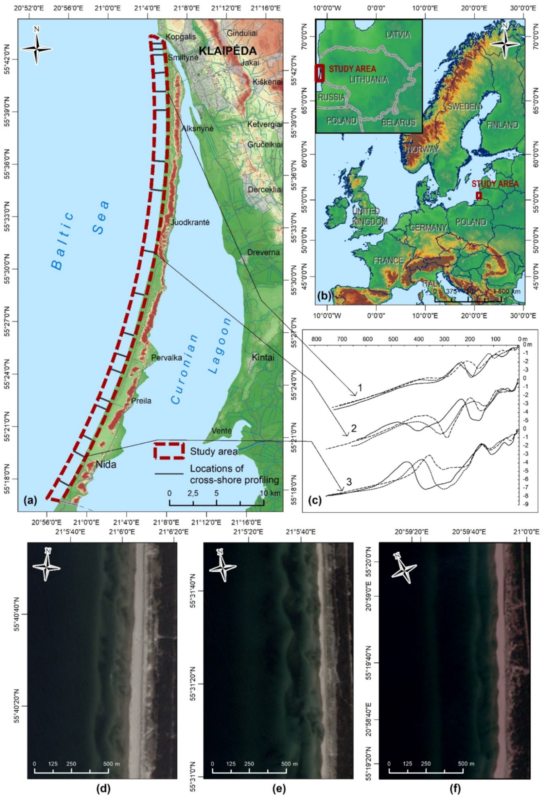
2.1. Study Area

The proposed algorithm has been tested in a sandy barrier—the Curonian Spit—separating Curonian Lagoon from the south-eastern Baltic Sea (Figure 1). The Curonian Spit politically is divided between Lithuania (51 km) and Russia (47 km); the Lithuanian part, stretching in the northeast from Nida settlement to Klaipėda port jetty, has been considered in this study. The coast of the Curonian Spit is a non-tidal (tidal range < 0.05 m) wave-dominated environment with predominant lower than 2.0 m waves approaching from western directions (NW, SW, W). The annual mean wave height at the Lithuanian Baltic Sea coast is 0.5–1 m [64]. Wave climate has a seasonal character with the occurrence of higher waves in autumn and winter (0.76 and 0.85 m) and lower waves in spring and summer (0.56 and 0.62 m) [65]. During storms, wave height may reach 4–6 m. Wave energy flux in a year of median wave intensity is equal to 1.21 kWh/m on average and depends on seasonality, reaching its maximum in winter (2.38 kWh/m) and minimum in summer (0.68 kWh/m) [65]. The net annual longshore sediment supply is directed northward. Subaerial coast is defined by 30-80 m wide beaches, composed of fine to medium sand and bordered by up to 16 m high foredune [66].

The nearshore is characterized by a gentle slope (tanβ = 0.009–0.015, up to 8 m water depth) with a multiple sandbar system consisting of 2–5 bars. The increasing number of sandbars and decreasing sandbar volume describe the variability of nearshore morphology from the southern to the northern end of the Curonian Spit. The sandbar zone with 10–400 m wide sandbars stretch from 250 to 750 m offshore. Sandbar crests rise 0.15–4.9 m above the trough in up to 5.6 m water depth over them. The sandbar system exhibits various morphologies from longshore straight to crescentic and shore-attached. According to Wright and Short [67], the morphology of inner bars are from the transverse bar and rip (TBR) to rhythmic bar and beach (RBB) and longshore bar and trough (LBT) states; outer bar morphology usually corresponds to longshore bar and trough (LBT) or dissipative (D) states. Complex sandbar morphologies complicate automated sandbar crest extraction in remote sensing images but also make the study area a suitable polygon to design and examine such an algorithm.

2.2. Satellite Data

Multispectral imagery of PlanetScope and RapidEye sensors, provided by Planet Labs Inc. under the Education and Research program [68], were used in this study.

RapidEye satellite system is a constellation of five identical five-band multispectral sensors (

Table 1. Specifications of the RapidEye and PlanetScope sensors and products used in this study.

Constellation	Sensor Type	Revisit Time	Spatial Resolution	Wavelength Range (nm)	Utilized Product	Pixel Value
PlanetScope	four-band frame imager	daily	3 m	Blue: 455–515 1 (464–517) 2 Green: 500–590 1 (547–585) 2 Red: 590–670 1 (650–682) 2 NIR: 780–860 1 (846–888) 2	PlanetScope Analytic Ortho Scene Product (Level 3B)	Surface reflectance
RapidEye	push-broom	5.5 days	5 m	Blue: 440–510 Green: 520–590 Red: 630–685 Red Edge: 690–730 NIR: 760–850	RapidEye Analytic Ortho Tile Product (Level 3A)	Surface reflectance

¹ first-generation satellites; ² second-generation satellites, launched starting in November 2018.

), operated in 2009–2020. PlanetScope satellite system is a constellation, also known as the Dove satellite constellation, launched in 2017. It comprises multiple launches of groups of individual CubeSat satellites (total approx.130 satellites) with multispectral four-band sensors daily acquiring data of the entire Earth land surface. The wavelength of PlanetScope bands varies depending on satellite generation (Table 1). In this study, RapidEye Level 3A and PlanetScope Level 3B data products (Table 1), both radiometrically corrected and orthorectified with Ground Control Points (GCPs) and elevation model (DEM) to <10 m RMSE positional accuracy, were analysed. RapidEye Level 3A products are distributed as constant 25 × 25 km² grid tiles. PlanetScope satellites collect imagery as overlapping framed scenes of size equal to 25 × 11.5 km² or 25 × 23 km², and scenes are not organized into a constant tiling grid system [69].

Both PlanetScope and RapidEye images were visually inspected, and only dates satisfying three criteria were selected. Criteria include cloud cover up to 20%, relatively clear water (sandbars are visible), no visible wave breaking over sandbars. Mean significant wave height on dates when selected images were acquired was 0–0.65 m (0.27 m on average), on dates used for algorithm validation between 0.07 and 0.4 m.

2.3. In Situ Data

Data of bathymetric surveys conducted with DualBeam Humminbird Helix 9 SI GPS echo-sounder, mounted on a shallow draft motor vessel, were used to validate sandbar crest position derived from satellite images. During surveys, dual beams of 200 kHz/ 20° and 83 kHz/ 60° were used. The echo-sounder blends returns from both frequency beams by starting with 83 kHz wide beam return (secondary source), dimming it, and then overlaying it with the 200 kHz narrow beam return (primary source). Echosounder has an integrated GPS/WAAS receiver, providing fast position fixes accurate within 2.5 m. Measurements were vertically corrected for water level fluctuation using data acquired with GNSS Topcon HiPer SR.

Bathymetric surveys are a result of cross-shore profiling along the Curonian Spit nearshore at 17 different locations with a spacing of 1–5 km (Figure 1). Surveys were performed in spring and autumn under low wave energy. Sandbar crests at six dates with 1–6 days difference between a bathymetric survey and image acquisition were compared with PlanetScope-derived crests and at four dates with 1–4 days difference with RapidEye-derived crests (

Table 2. The dates of PlanetScope and RapidEye images used for sandbar crest extraction compared with the dates of bathymetric surveys used for accuracy evaluation of satellite-derived crest positions.

Constellation	Date of Image Acquisition	Date of Bathymetric Survey
PlanetScope	29 September 2017	29–30 September 2017
PlanetScope	16 May 2018	16 May 2018
PlanetScope	11 October 2018	12 October 2018
PlanetScope	22 May 2019	18–19 May 2019
PlanetScope	26 September 2019	26–27 September 2019
PlanetScope	26 June 2020	20 June 2020
RapidEye	1 October 2017	29–30 September 2017
RapidEye	20 May 2018	16 May 2018
RapidEye	15 October 2018	12 October 2018
RapidEye	22 May 2019	18–19 May 2019

).

2.4. Data Pre-Processing

Multiple scenes of analysed sensors cover the study area (RapidEye—4 scenes; PlanetScope—variable number of scenes). Scenes were composed into mosaics covering all of the study area prior to further processing and analysis. PlanetScope multi-band mosaics were resampled to 5 m/pixel spatial resolution using bilinear interpolation to eliminate the difference between PlanetScope and RapidEye sensors. Enhanced Lee filter with the kernel of 3x3 pixels (Section 2.5) was applied to RapidEye mosaics prior to processing to reduce noise-induced distortions.

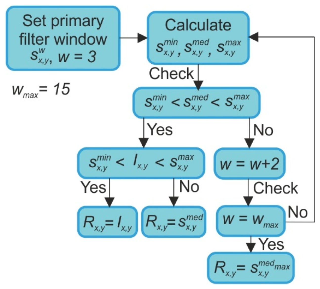
2.5. Spatial Filtering

The quality of PlanetScope and RapidEye images used in this study suffers from low signal-to-noise ratios compared to other optical sensors [70,71,72,73,74]. By distorting the original signal, noise complicates the process of sandbar extraction and causes sandbar fragmentation during the procedure. To solve this problem, spatial filtering techniques—adaptive median, enhanced Lee, Kuan and Gaussian filters—applied at different stages of the sandbar extraction procedure are presented.

In this study, a modified version of the adaptive median filter suggested by Li and Fan [75] was applied (Figure 2). Filter reduces the variance of intensities in the image by replacing pixel value with a median value within the defined window surrounding the processing pixel. The window surrounding each pixel is variable, and it is determined whether the pixel is noisy in a current window prior to changing its value.

The Enhanced Lee filter—introduced by [76] as an improvement of Lee filter [77] categorizes pixels into three classes: homogenous, heterogeneous and point target [76]. The distinction of classes relies on the image variation $C_i$, noise variation $C_u$ and maximum noise variation $C_{max}$ coefficients. In image $I_{x,y}$, the signal $R_{x,y}$ is expressed as in Equation (1):

$$R_{x,y}=\{\begin{array}{c}\overline{I_{x,y}}, for C_i\le C_u\\ I_{x,y}\times W_{x,y}+I_{x,y}\times \left(1-W_{x, y}\right),\\ I_{x,y}, for C_i\ge C_{max}\end{array}for C_u<C_i<C_{max}$$

(1)

where $W_{x,y}$ is weighting function.

The Kuan filter is an adaptive filter for speckle noise reduction introduced by Kuan et al. [78]. In the Kuan filter, a multiplicative model is transformed to a signal-dependent additive noise model and the pixel value is smoothed using an estimate from the local mean, variance and standard deviation (Equation (2)):

$$R_{x,y}=I_{x,y}\times W_{x,y}+I_{x,y}\times \left(1-W_{x,y}\right)$$

(2)

where $W_{x,y}$ is weighting function.

Although the Enhanced Lee and Kuan filtering techniques are typically utilized to despeckle radar images, optical images used in this study portray a granular appearance different in nature but visually similar to multiplicative speckle radar noise, and local statistics filters effectively reduce such graininess and image fragmentation caused by it.

The Gaussian filter is a low-pass convolution filter, where an image $I_{x,y}$ is multiplicated by convolution matrix (kernel) K, which is a discrete approximation of the Gaussian function. In this study, a kernel of 5 × 5 pixels was used as in Equation (3).

$$\mathrm{K}=\frac{1}{256}\left[\begin{array}{ccccc}1& 4& 6& 4& 1\\ 4& 16& 24& 16& 4\\ 6& 24& 36& 24& 6\\ 4& 16& 24& 16& 4\\ 1& 4& 6& 4& 1\end{array}\right]$$

(3)

2.6. Algorithm for Sandbar and Sandbar Crest Extraction

The proposed algorithm is divided into four stages of data processing and analysis. First, a shoreline is extracted, and a land-sea mask is created to discriminate the subaqueous domain with nearshore sandbars from the subaerial domain (the detailed procedure is discussed in Section 2.6.1). Second, multiple calculations are performed in the subaqueous domain to generate raster, representing nearshore bottom morphology, where sandbars and their crestlines might be identified easily (Section 2.6.2). Then, in a generated raster, boundaries of nearshore sandbars are defined, and sandbars are extracted (Section 2.6.3). Finally, sandbar crestlines are derived within previously defined boundaries (Section 2.6.4).

The algorithm was implemented in a GIS environment (ArcGIS Desktop 10.7). Maximum value pixels per transect was extracted via a script written in the R programming language. The script was made available as a tool in ArcGIS via an R-ArcGIS bridge.

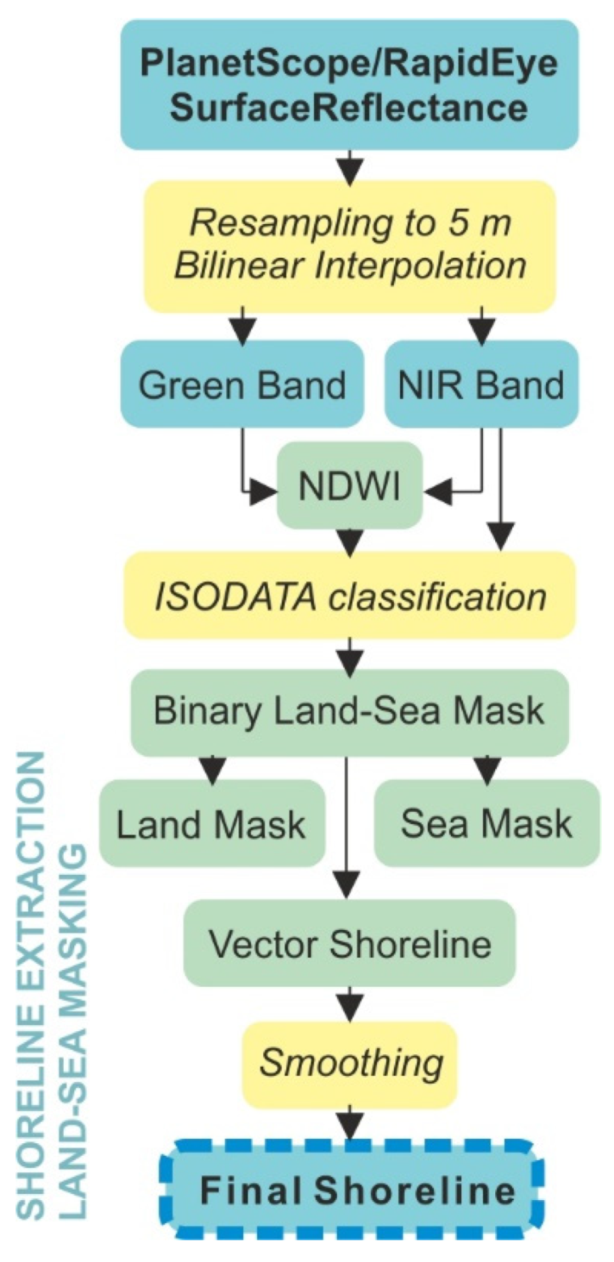
2.6.1. Land-Sea Masking and Shoreline Extraction

The land-sea masking procedure is based on spectral differences between water and land in infrared bands where water absorbs most of the radiation. Many spectral indices for water retrieval have been introduced based on this reflective property [51,79,80,81]. Most of them are combinations of the visible light spectrum and near-infrared (NIR) or short-wave infrared (SWIR) wavelengths. Because PlanetScope and RapidEye sensors contain a limited number of bands with only near-infrared outside visible light spectrum, Normalized Difference Water Index (NDWI) [79] (requiring only green and near-infrared reflectance) was employed in water and land separation procedure. It was calculated using Equations (4) and (5) for PlanetScope and RapidEye sensors, respectively.

$$NDW{I}_{PlanetScope}=\frac{S{R}_2-S{R}_4}{S{R}_2+S{R}_4}$$

(4)

where SR₂ and SR₄ correspond to the surface reflectance of the green and near-infrared bands of the PlanetScope sensor.

$$NDW{I}_{RapidEye}=\frac{S{R}_2-S{R}_5}{S{R}_2+\mathrm{S}{R}_5}$$

(5)

where SR₂ and SR₅ correspond to the surface reflectance of the green and near-infrared bands of the RapidEye sensor.

NDWI was designed with a 0 threshold to distinguish water and land, but this value varies depending on sensor and image properties. Although several methods have been tested for binarization of NDWI images (0 thresholding, Otsu thresholding), The Iterative Selforganizing Data Analysis Techniques Algorithm (ISODATA) was chosen to derive land-sea masks and delineate shoreline. NDWI and near-infrared band images were used as inputs for ISODATA unsupervised classification. Employing both NDWI and near-infrared band images gave more stable results in most instances compared to NDWI alone. The main steps of the land-sea masking and shoreline delineation procedure are shown in Figure 3.

2.6.2. Generation of Inputs for Sandbar and Sandbar Crest Extraction

In bands of the visible light spectrum, brighter pixels with larger reflectance values represent shallower underwater features. Therefore, surface reflectance values might be considered relatively representative of the bathymetric position. In geomorphology, a topographic position might be described by topographic indices, which compare the elevation of central pixel to elevations within the local neighbourhood, defined by window size [82]. These metrics are typically used for landform classification [83,84,85,86], but they deal with the same issue as this study—distinguishing positive landforms from negative or sandbars from troughs. The most applied metric of local topographic position is the Topographic Position Index (TPI), in marine geomorphology referred to as the Bathymetric Position Index (BPI) [87]. It is a signed unbounded absolute metric comparing the elevation of the central pixel with a mean elevation in a local neighbourhood. Similarly, the Relative Topographic Position Index (RTPI), which links central elevation with mean, minimum and maximum values within the local neighbourhood, was introduced. It is a signed metric accounting for elevation distribution, bounded by the interval (–1,1). As this paper deals with subaqueous features, it will be further referred to as the Relative Bathymetric Position Index (RBPI).

Both the BPI and the RBPI have been examined in this study. As surface reflectance decreases with increasing water depth and distance offshore, inner sandbars are represented by higher surface reflectance values than outer sandbars despite their height. Using an absolute metric as the BPI results in sinking outer sandbars because of a smaller difference between values in the local neighbourhood. Using a relative metric as the RBPI, which considers minimum and maximum values in the local neighbourhood, reduces distortions caused by water depth over sandbar crest and results in a better representation of nearshore morphology. Hence, the RBPI was chosen for further analysis. It was calculated separately for blue, green and red bands of PlanetScope and RapidEye imagery, using Equation (6) (based on Newman, Lindsay and Cockburn [82].

$$RBPI=\{\begin{array}{c}\frac{SR- S{R}_{mean}}{S{R}_{mean}- S{R}_{min}} if SR<S{R}_{mean}\\ \frac{SR-S{R}_{mean}}{S{R}_{max}-S{R}_{mean}} if SR>S{R}_{mean}\end{array}$$

(6)

where SR denotes surface reflectance of the processing pixel and SR_mean, SR_min and SR_max denote mean, minimum and maximum surface reflectance values in the local neighbourhood, respectively.

The RBPI depends on the size of the local neighbourhood. Choice of the window size determines the scale at which underwater landforms is distinguished: using small-sized window results in a detailed picture of smallest-scale underwater features and fragmented large-scale landforms (Figure 4b); large-sized window results in distinguished large-scale underwater landforms with small-scale features merged into the whole (Figure 4e). In multiple nearshore sandbar systems, spacing and scale of submerged sandbars increase in the offshore direction [5,35,88]. Therefore, the optimal size of the local neighbourhood for inner and outer sandbars diverges. To save all the information about inner and outer sandbars multiscale approach for RBPI calculation is implemented. The routine of this approach is presented below and in Figure 5.

Procedure for the multiscale RBPI computation:

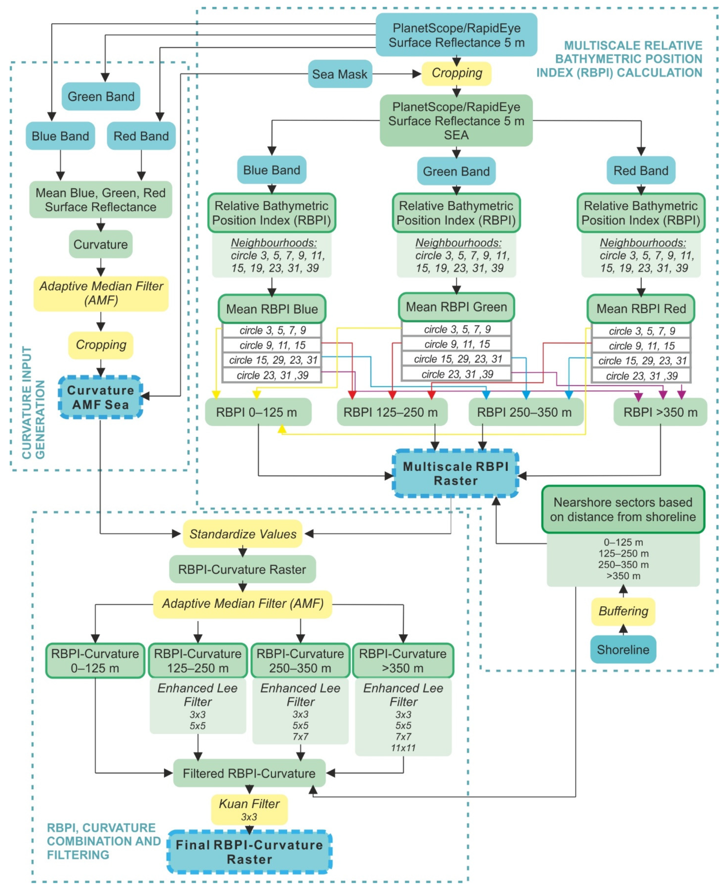
• Nearshore zone is divided into fixed cross-shore sectors based on offshore distance (Figure 4a). The width and number of the cross-shore sectors are defined by prevailing features of the sandbar system in the study area.
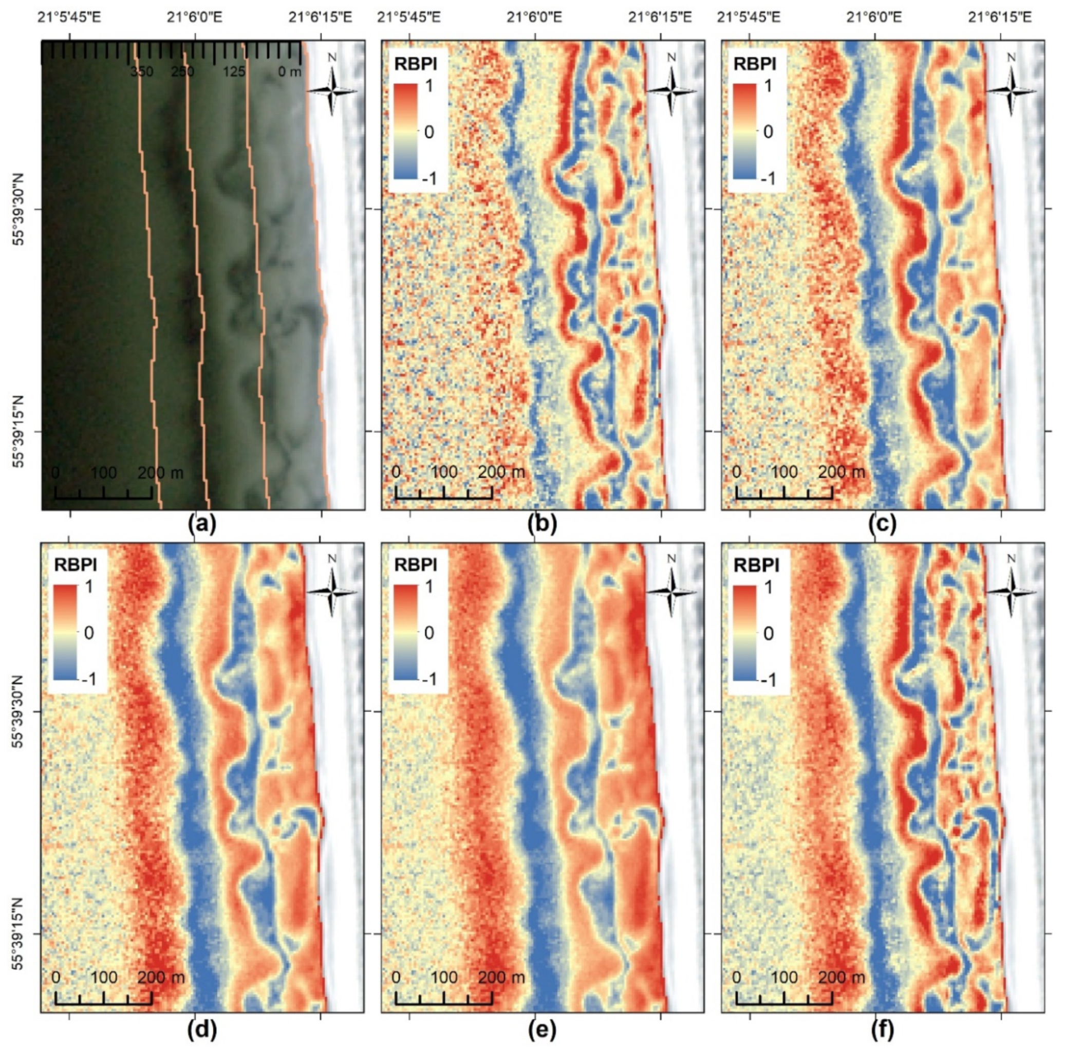
• RBPI values with 10 circle local neighbourhoods (Figure 5) are calculated for visible light bands. The motive for the choice of a circle neighbourhood instead of the traditional square was a continuous and smooth nature of nearshore sandbar shape.
• The mean of RBPI values in local neighbourhoods of multiple sizes was calculated for each sector in each band of the visible light spectrum: from the mean of 3 smallest neighbourhoods for the sector closest to the shoreline to the mean of 3 largest neighbourhoods for the sector furthest offshore (Figure 5). Other measures of descriptive statistics have been tested, and the maximum value was considered instead of the mean, but it resulted in random noise generation.
• Mean RBPI values in local neighbourhoods of multiple sizes for nearshore zone sectors in blue, green and red bands are summed using weighting coefficients. The selection of weighting coefficients was mainly governed by the penetrating capabilities of blue, green and red light and the quality of band images. In coastal waters, green light penetrates the water column the deepest [89], and the sandbar system is visible most sharply in its image. In contrast, longer red wavelengths are quickly absorbed by water, and only inner-middle sandbars are completely visible in their images, whereas the outer sandbar is often obscure. Blue wavelengths penetrate the water column deeper than red, but their images contain significant distortions caused by noise in both PlanetScope and RapidEye mosaics. Therefore, the largest coefficient of 0.6–0.8 was given to the green band; a coefficient of 0.1–0.3 was given to the red band; 0.1–to the blue band. The proportion of coefficients for green and red bands was differentiated based on nearshore cross-shore sectors: as distance offshore increases, the coefficient for green band increases. Final RBPI values for nearshore cross-shore sectors are calculated as in Equation (7):

$$\{\begin{array}{c}0.1\times {\mu }_{RBPIBlue }+0.6\times {\mu }_{RBPIGreen }+0.3\times {\mu }_{RBPIRed } if D_{off} <250 \mathrm{m}\\ 0.1\times {\mu }_{RBPIBlue }+0.7\times {\mu }_{RBPIGreen }+0.2\times {\mu }_{RBPIRed } if 250 \mathrm{m}<D_{off} <350 \mathrm{m}\\ 0.1\times {\mu }_{RBPIBlue }+0.8\times {\mu }_{RBPIGreen }+0.1\times {\mu }_{RBPIRed } if D_{off} >350 \mathrm{m}\end{array}$$

(7)

where µ_Blue, µ_Green and µ_Red denote mean RBPI values in multiple sizes local neighbourhoods for blue, green and red bands of PlanetScope and RapidEye imagery, and $D_{off}$ denotes the distance from the shoreline. The result is saved as a multiscale RBPI Raster (Figure 6b).

The multiscale RBPI is calculated only for the underwater part of an image. When there is no shore-attached sandbar, a step or a slight slope is a typical characteristic of foreshore. The upper slope of the foreshore is characterized by higher surface reflectance values than the lower one. When RBPI is calculated, it might be misclassified as a positive landform (sandbar). To solve this issue, the multiscale RBPI Raster is combined with a second-order derivative raster, which represents surface curvature (convexity and concavity). In the Curvature raster, the foreshore is a convex surface, and in combination with multiscale RBPI Raster, the Curvature raster submerges the misleadingly elevated upper slope of the beach face. The routine of Curvature generation and combination with the multiscale RBPI is described below and in Figure 5.

The multiscale RBPI and Curvature combination procedure:

• The mean surface reflectance value for blue, green and red bands is calculated.
• Mean surface reflectance raster of blue, green and red bands is used as an input for the second-order derivative (further curvature) calculation.
• Curvature raster is clipped to the submerged part only and filtered with an adaptive median filter (Section 2.5). It reduces random multiplicative noise in curvature images without oversmoothing of data. The result is saved as Curvature AMF Sea Raster (Figure 6c).
• Values of the Curvature AMF Sea and multiscale RBPI rasters are standardized and summed as in Equation (8):

$${\mathrm{RBPI}}_{\mathrm{stand}}+0.3\times {\mathrm{Curvature}}_{\mathrm{stand}}$$

(8)

where ${\mathrm{RBPI}}_{\mathrm{stand}}$ and ${\mathrm{Curvature}}_{\mathrm{stand}}$ denote standardized values of the multiscale RBPI and Curvature AMF Sea rasters, respectively. Combined multiscale RBPI and Curvature rasters are saved as the RBPI-Curvature raster.

Noise-induced segmentation and cross-shore differences in scale and distinctiveness of sandbars define the need to apply smoothing of different intensities to RBPI-Curvature raster in previously distinguished nearshore cross-shore sectors. To accomplish this, an Enhanced Lee filter (Section 2.5) with multiple window sizes (3 × 3; 5 × 5; 7 × 7; 11 × 11) is applied (Figure 5). At first, random multiplicative noise is reduced in the RBPI-Curvature raster with an adaptive median filter (Section 2.5), then an Enhanced Lee filter with 3 × 3 window is applied to the RBPI-Curvature raster after adaptive median filtering; 5 × 5 Enhanced Lee filter is applied to raster after 3 × 3 filtering, 7 × 7 after 5 × 5 and 11 × 11 after 7 × 7 to obtain rasters with increasing level of smoothing. As the offshore distance increases, the output of filtered RBPI-Curvature raster with a greater degree of smoothing is assigned to cross-shore distance-based nearshore sectors and combined into a single output (Figure 5). Finally, differences at edges of combined outputs are smoothed with Kuan filter (Section 2.5) with a 3 × 3 window. It was chosen because the Kuan filter does not categorize pixels as the Enhanced Lee filter (which better preserves edge sharpness) and gives the result with more naturally smoothed edges. The result after the filtering procedure is furthered referred to as Final RBPI-Curvature raster (Figure 6d).

To sink non-bar regions and to expose sandbars Final RBPI-Curvature raster is rescaled to scale from 1 to 1000 with MSLarge transformation function (Figure 7). MSLarge function brings out large values based on the mean and standard deviation of data. After transformation, deeper non-sandbar nearshore regions remain only as background with the same value, and higher regions of the nearshore bottom with sandbars preserve all range of values ($\mathrm{non}-\mathrm{sandbar} \mathrm{region}=1;$ $1<\mathrm{sandbar} \mathrm{region}\le 1000$). Rescaled RBPI-Curvature raster values are converted to an integer, and a Majority filter with an 8-pixel neighbourhood is applied to remove the remaining small regions with a few isolated pixels to get a cleaner result. In this instance, if Rescaled RBPI-Curvature raster has remaining isolated pixels, they are replaced with background value because the majority filter replaces pixel value with mode if 5 out of 8 contiguous pixels have the same value. Rescaled RBPI-Curvature raster (Figure 6e) is the final output for the extraction of nearshore sandbars.

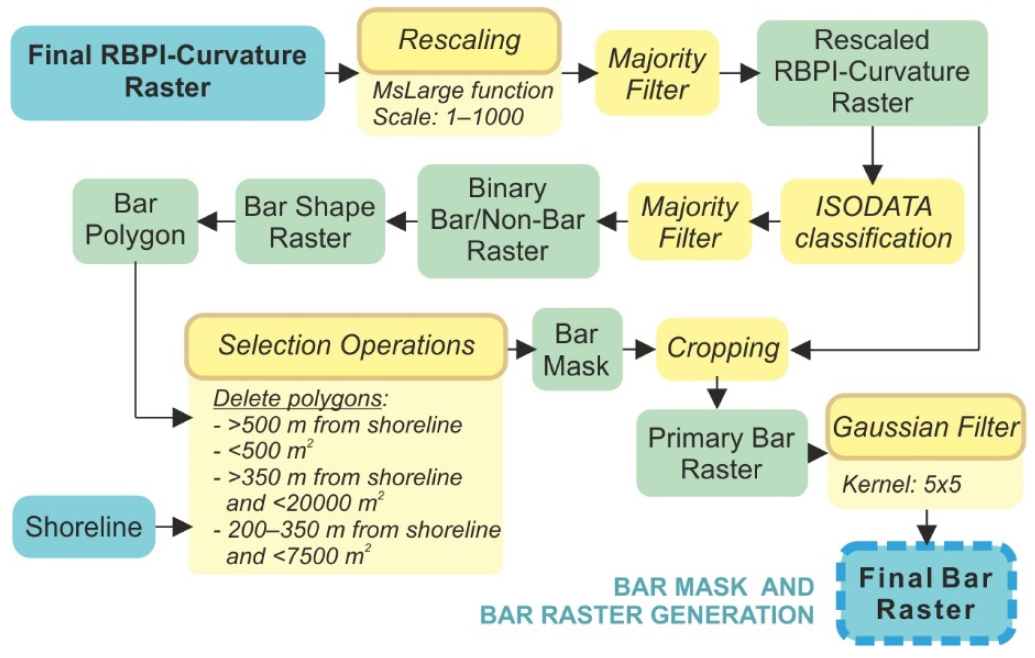
2.6.3. Extraction of Nearshore Sandbars

A rescaled RBPI-Curvature raster is used as an input for nearshore sandbar extraction. It is classified into two classes—sandbar and non-sandbar regions—with ISODATA unsupervised clustering. Classified raster is filtered with majority filter twice to remove remaining isolated pixels and to get a cleaner boundary of sandbars, and then the class with non-sandbar regions is set to no-data, and an integer raster with sandbars only is generated. It has remaining misclassified areas mostly outside the sandbar zone where surface reflectance values in the primary image were uneven due to noise signal, thin clouds, haze and heterogeneity of water surface. To remove misclassified regions, the sandbar raster is converted to a vector polygon layer, which is cleaned using selection operations with defined criteria based on the typical distance from the shoreline $D_{off}$ and size of sandbars $A$ in the study area. The details of the criteria are described below and in Figure 7.

The criteria to eliminate non-sandbar regions misclassified as sandbars:

• $D_{off}>500 \mathrm{m}$ (typically, the inner boundary of outer sandbars is within 500 m from the shoreline at least at one of its segments in the Curonian Spit)
• $A<500 {\mathrm{m}}^2$
• $D_{off}>350 \mathrm{m}$ and $A<20,000 {\mathrm{m}}^2$
• $200 \mathrm{m}<D_{off}<350 \mathrm{m}$ and $A<7500 {\mathrm{m}}^2$.

If a polygon satisfies at least one criterion, it is deleted as a non-sandbar. All remaining polygons are considered as sandbars and are saved as Bar Mask (Figure 6f). The rescaled RBPI-Curvature raster is clipped with Bar Mask and saved as Primary Bar Raster.

To smooth the Primary Bar Raster and to ensure the continuity of sandbar crests after the extraction Gaussian filter with a 5 × 5 kernel (Section 2.5) is applied. The result is saved as Final Bar Raster (Figure 6g). Additionally, the Slope was calculated for the Final Bar Raster, then inverted and saved as Bar-Slope Raster. The Slope is calculated as the maximum change in value over the distance between a pixel and its eight neighbours It was not employed in further process, but it provides an output of extracted sandbars with clearly visible crestline (Figure 6h).

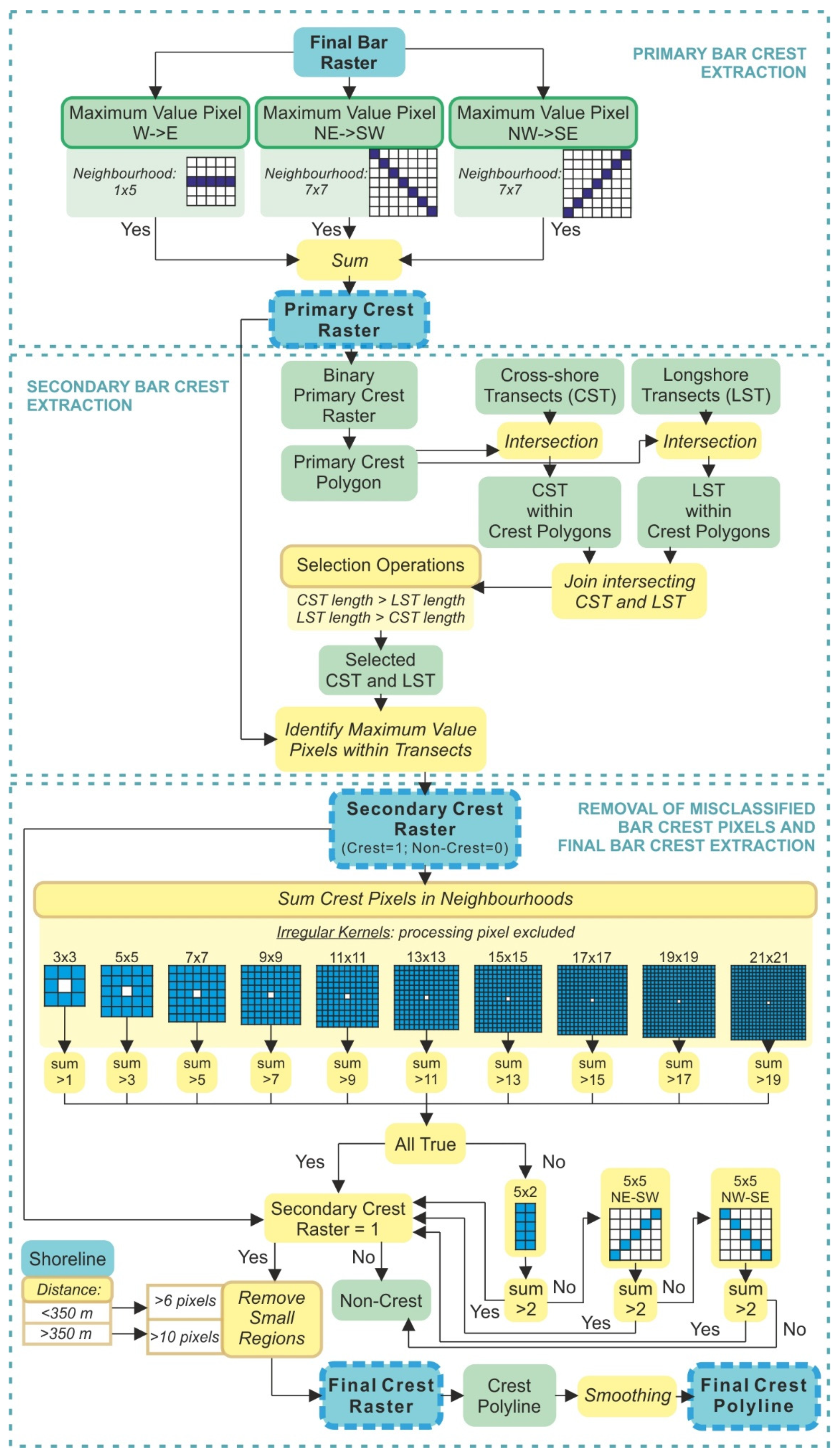
2.6.4. Extraction of Nearshore Sandbar Crests

Complex sandbar morphologies (crescentic shapes, rhythmic patterns, etc.) determines that sandbar crestlines might exhibit variable shapes and orientation relative to the shoreline: parallel, oblique or transverse. The typical approach to detect longshore sandbar crest locations with shoreline-perpendicular transects (e.g., [62]) might not identify all the variability of sandbar crestline shapes leading to undetected or incorrectly delineated crests that are not parallel to the shoreline. For better detection of sinuous crestlines, they are located in three directions: perpendicular to the shoreline and oblique to the shoreline (at 45°–225° and 135°–315° angles). Because the main shoreline direction in the study area is orientated from south to north, these directions correspond to West-East (W–E), North East–South West (NE–SW) and North West–South East (NW–SE) orientations.

In the crestline delineation procedure, maximum value pixels within local neighbourhoods defined by the rowing window in the Final Bar raster are considered as crests. Three local neighbourhoods, which represent perpendicular and oblique directions, are utilized (Figure 8):

• A local neighbourhood with 5 pixels (25 m) orientated in the W–E direction;
• An irregular local neighbourhood with 7 pixels (35 m) in the NE–SW direction (35 m in an oblique direction is equivalent to 25 m in a perpendicular direction of the same 25 × 25 m square neighbourhood);
• An irregular local neighbourhood with 7 pixels (35 m) in the NW–SE direction.

Figure 8. A flowchart of the sandbar crest extraction procedure: at first, the primary crest as maximum value pixels within three kernels are identified, then secondary crest with cross-shore/longshore transects is extracted, and the final bar crest is obtained after cleaning procedure with proximity-based filter.

Figure 8. A flowchart of the sandbar crest extraction procedure: at first, the primary crest as maximum value pixels within three kernels are identified, then secondary crest with cross-shore/longshore transects is extracted, and the final bar crest is obtained after cleaning procedure with proximity-based filter.

If it is indicated that pixel value is equal to maximum within W–E, NE–SW, or NW–SE neighbourhood, it is considered as crest candidate. Identified maximum pixel values within all three neighbourhoods are summed. Here, if the same pixel has maximum value within multiple neighbourhoods, it will be attributed with a higher value than pixels with maximum value within one neighbourhood. Raster with summed maximum pixel values within W–E, NE–SW and NW–SE directed neighbourhoods is considered the Primary Crest Raster (Figure 6i).

If maximum value pixels do not match within all local neighbourhoods, a crest wider than one pixel is generated in the Primary Crest Raster. To narrow crestlines to one pixel-wide maximum value pixels, secondary crests within crests candidate pixels in the Primary Crest Raster are determined using cross-shore (CST) and longshore (LST) transects. The procedure of secondary crest extraction is described below and in Figure 8.

The procedure for secondary crest extraction:

• Primary Crest Raster is binarized and converted to polygon layer (Primary Crest Polygon).
• Cross-shore (CST) and longshore (LST) transects with spacing equal to satellite image resolution (5 m) are created and intersected with Primary Crest Polygon.
• Intersecting CST and LST within primary crest polygons are joined based on their spatial relationship.
• Lengths (d) of pairs of intersecting CST (${\mathrm{d}}_{\mathrm{CST}}$) and LST (${\mathrm{d}}_{\mathrm{LST}}$) are compared: if ${\mathrm{d}}_{\mathrm{CST}}>{\mathrm{d}}_{\mathrm{LST}}$, it is considered that the main sandbar crest direction is orientated parallel to the shoreline, and CST is selected; if ${\mathrm{d}}_{\mathrm{CST}}<{\mathrm{d}}_{\mathrm{LST}}$, the main sandbar crest direction is orientated perpendicular to the shoreline, and LST is selected; if ${\mathrm{d}}_{\mathrm{CST}}={\mathrm{d}}_{\mathrm{LST}}$, CST is selected. Selected CST and LST are merged into one layer. CST and LST lengths are equal when crests in Primary Crest Raster are one-pixel wide (in most instances), and CST/LST selection makes no difference because, in any case, the same pixel will be the maximum value pixel.
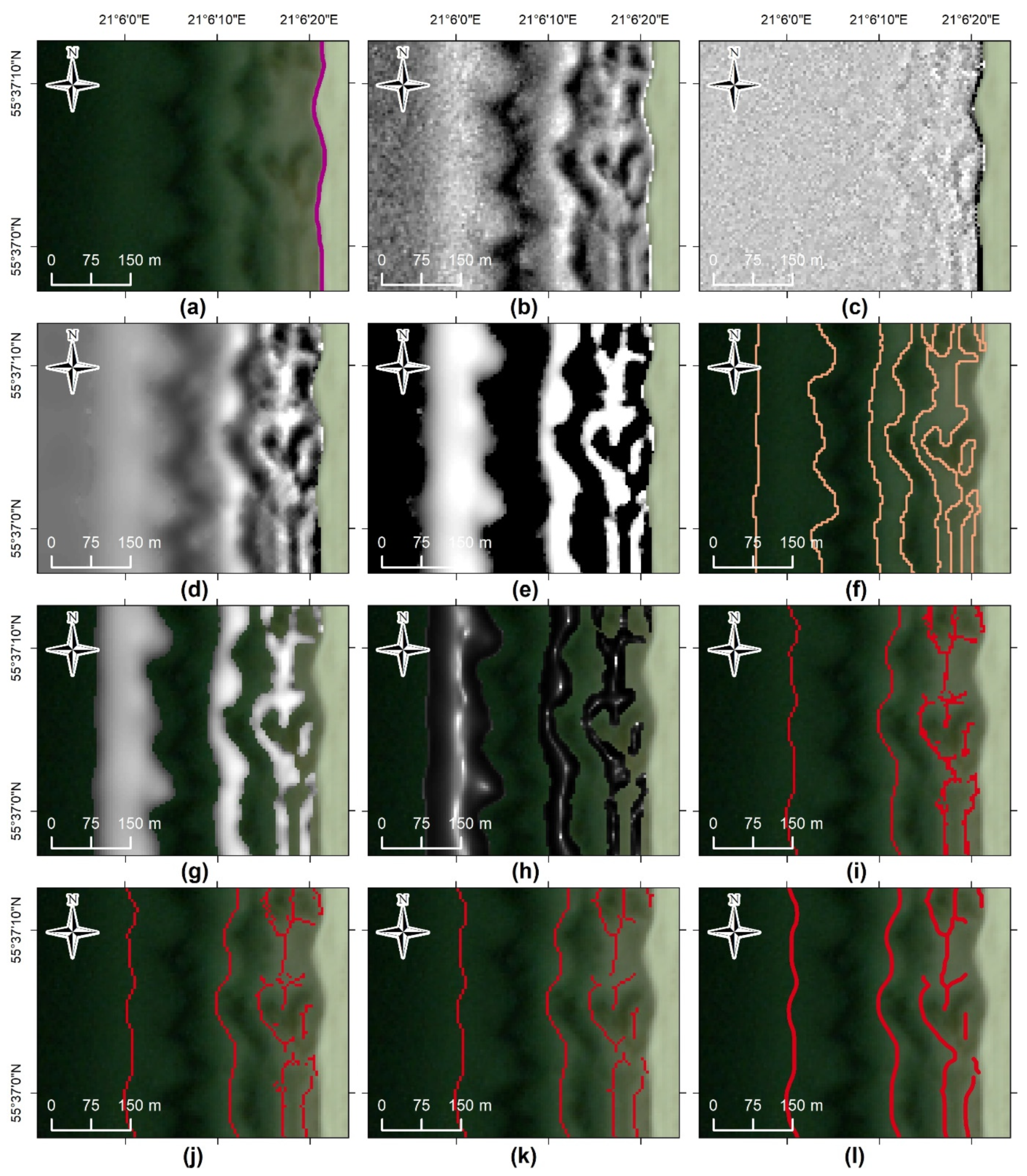
• Maximum value pixels within selected CST and LST transects are identified as secondary crest pixels and exported to Secondary Crest Raster (Figure 6j).

The Secondary Crest Raster has remaining non-crest pixels misclassified as crests (usually sandbar boundary pixels or other redundant pixels/pixel regions). To distinguish them from actual crests, a crest cleaning algorithm is implemented. It is based on the understanding that the sandbar extends at least tens of meters, and one or a few isolated pixels cannot represent the sandbar crestline. It means that the crest pixel must have a certain number of neighbours also identified as crests. Local neighbourhoods of increasing size with the defined requirement for the number of neighbours to be crest pixels were used as a part of the crest cleaning algorithm. The details of the routine are described below and in Figure 8.

The routine for crest cleaning:

• Square kernels with excluded centre (processing) pixels are used to quantify the number of neighbourhood pixels. Minimal kernel size is 3 × 3 pixels (15 × 15 m), and the maximum is 21 × 21 (105 × 105 m). Every kernel is expanded by 2 pixels until the maximum is reached. Crest values in the secondary crest raster are set to 1, so that sum of values in the kernel would be equal to the number of crest neighbours (Figure 8).
• It is determined that in a neighbourhood of 3 × 3 pixels, processing crest pixel must have at least 2 crest neighbours (sum > 1). It means that within 8 neighbour pixels, at least 2 must be sandbar crests. When the kernel is expanded by 2 pixels, the requirement of the sum in the neighbourhood is also increased by 2 (Figure 8). The process is repeated until the maximum kernel is reached.
• A pixel is identified as crest only if the requirement of the sum is fulfilled in all kernels, and it was previously identified as a crest pixel (value in secondary crest raster was equal to 1).
• A defined filter sometimes is too aggressive and removes actual crest pixels, especially those at the beginning and at the end of the crestline or when the crest is sinuous. Thus, part of filtered pixels is restored with three kernels: 5 × 2 pixels square; 5 pixels NE–SW and NW–SE directed (Figure 8). If the sum within at least one of three kernels is greater than 2, the pixel is restored as a crest pixel. If the pixel does not meet the criteria in all kernels, it is removed as a non-crest pixel.
• After filtering, small regions with aggregated pixels remain misclassified as crests. They are removed based on the number of pixels aggregated into one continuous region ($R$). Defined criteria are split based on distance from shoreline ($D_{off}$): if $D_{off}<350 \mathrm{m}$, $R<6 pixels$ are removed; if $D_{off}>350 \mathrm{m}$, $R<10 pixels$ are removed. Distance criterion is set because near the shoreline sandbar morphologies of smaller-scale form, while outer sandbar exhibits much greater extents, so aggregated regions must be larger to be considered as crests.
• After the removal of small regions, Final Crest Raster (Figure 6k) is created.
• The Final Crest Raster is converted to a polyline layer. Polylines are smoothed with 20 m smoothing tolerance and exported as Final Crest Polyline (Figure 6l).

3. Results

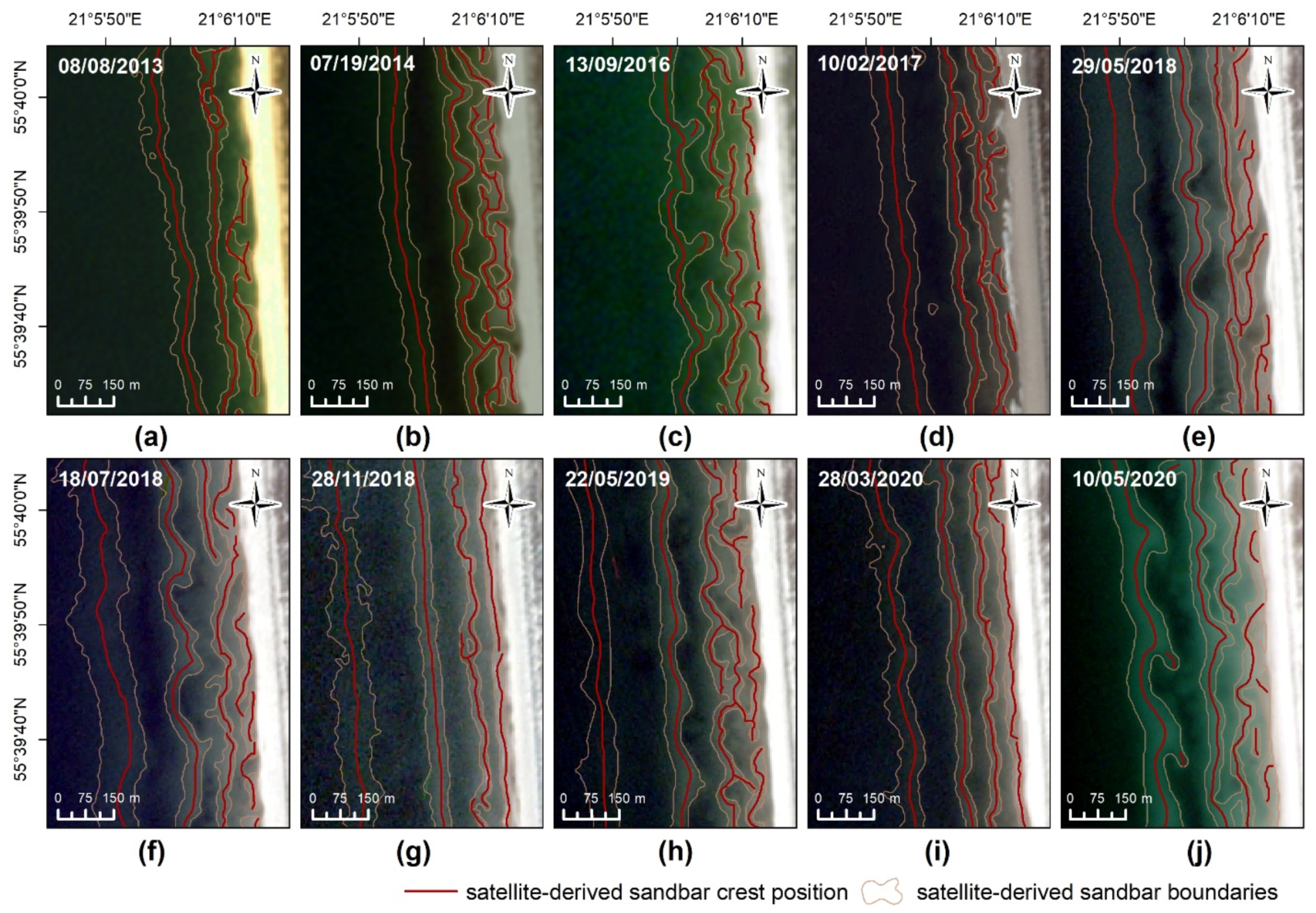
3.1. Visual Assessment of Extracted Sandbars

The proposed method has been tested with 42 RapidEye and 103 PlanetScope images acquired in 2009–2020. Extracted sandbars and their crests were visually inspected to assess the quality of results and possible shortcomings of the designed algorithm. Figure 9 shows an example of a time series with derived boundaries and crests of nearshore sandbars. Typical inter-annual characteristics of cyclic behaviour and seasonal patterns of morphological development in multiple sandbar systems are apparent here.

Although the algorithm was designed for images with clear water and calm sea, the visual assessment showed that sea surface roughness caused by small waves has no significant impact on the result of satellite-derived sandbar crests. Visual observations revealed that capabilities to detect less distinctive sandbars in greater depths decrease if the transparency of the water column or atmosphere is decreased by turbulency of sediment, haze, thin clouds, or other phenomena.

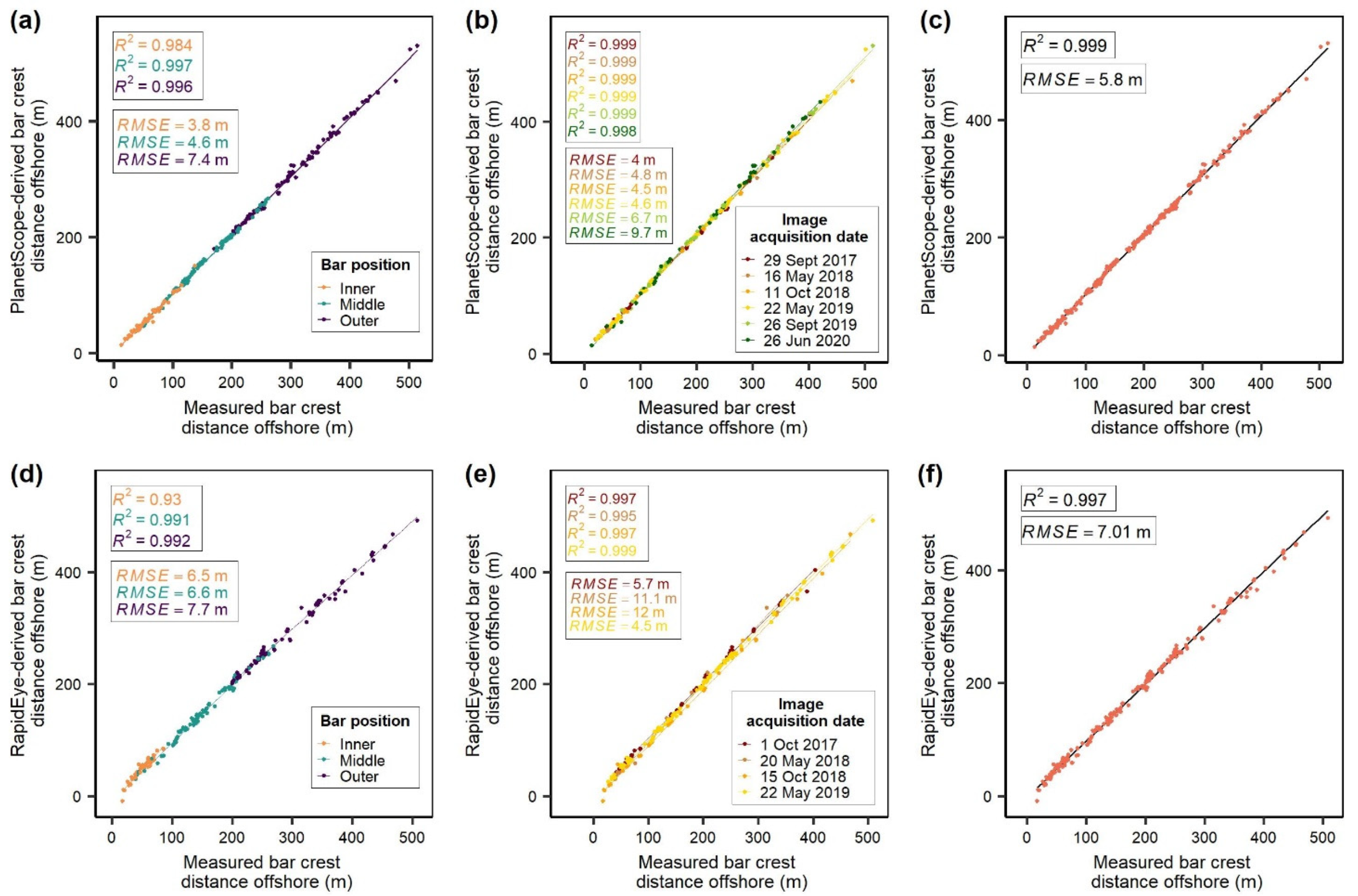
3.2. Accuracy of Extracted Crestline Position

Six pairs of PlanetScope images and bathymetric surveys with 332 pairs of crest positions were compared to validate the proposed method (Figure 10a–c). PlanetScope-derived sandbar crest locations are in good agreement with in situ data: the total coefficient of determination (R²) between measured and PlanetScope-derived sandbar crest distance from the shoreline was 0.999, ranging from 0.998 to 0.999 for individual dates. The root-mean-square error (RMSE) for all dates was 5.8 m, ranging from 4 to 9.7 m for individual dates (Figure 10b). For four out of six dates, RMSE was between 4 and 4.8 m, and only two dates showed errors larger than 5 m. The largest RMSE was for the image acquired on 26 June 2020, which had the largest time span between in situ and satellite data. Therefore, lower accuracy might be caused by changes in the sandbar system but not the algorithm itself.

Four pairs of RapidEye images and available bathymetric surveys with 231 pairs of crest positions were compared to validate the proposed procedure for this sensor (Figure 10d–f). RapidEye-derived sandbar crest locations are in good agreement with in situ data with the total coefficient of determination (R²) of 0.997, ranging from 0.995 to 0.999 for individual dates. The root-mean-square error (RMSE) for all dates was 7.01 m (Figure 10f). RMSE for two dates was between 4.5 and 5.7 m, and for the other two, between 11.1 and 12 m (Figure 10e), showing large inconsistencies among accuracy of individual dates. Visual comparison of the PlanetScope image acquired on the same day as the bathymetric survey and the RapidEye image acquired on 20 May 2018, with a 4-day time span from in situ measurements revealed that the shape of sandbars has evolved during this period. Visual inspection of the PlanetScope image obtained on 11 October 2018 (RMSE = 4.5 m), RapidEye image obtained on October 15 (RMSE = 12 m), and crest points from a bathymetric survey performed on 15 October has shown that the RapidEye image was shifted landward from measured crest points and the PlanetScope image. These observations suggest that deviations of errors are rather caused by morphodynamics of sandbars and errors in image positional accuracy.

The RMSE for inner, middle and outer sandbars in PlanetScope images was 3.8, 4.6 and 7.4, respectively (Figure 10a). The tendency of accuracy to increase as sandbar distance from shoreline decreases in RapidEye images remained similar as for PlanetScope sensor with RMSE of 6.5, 6.6 and 7.7 for inner, middle and outer sandbars, respectively (Figure 10d). The largest RMSE value for outer sandbar is because of the larger depth over their crests and the flat, wide shape of the crest itself, especially with the cases when outer sandbars are decaying.

The mean bias of sandbar distance offshore for PlanetScope and RapidEye sensors was 3.95 m and −2.71 m, respectively, meaning that sandbar distance from the shoreline in PlanetScope images was bias seaward and bias landward in RapidEye images. This tendency was evident for all individual dates. It suggests that data extracted from PlanetScope and RapidEye sensors in combination should be analysed with caution.

3.3. Accuracy of Extracted Shoreline Position

129 measured shoreline points were compared to PlanetScope-derived and 80 points to RapidEye-derived shoreline position to evaluate the accuracy of the proposed procedure for the shoreline extraction. The root-mean-square error (RMSE) for PlanetScope was 4.5 m, ranging from 0.2 to 7.7 m for individual dates. For RapidEye, the average RMSE was 4.4 m, ranging from 0.8 to 6.5 m for individual dates. In images of both sensors, the shoreline was placed seaward from the measured position with a mean bias of 3.9 m and 3.4 m for PlanetScope and RapidEye, respectively. Seaward-directed displacement of satellite-derived shoreline position is often observed in optical remote sensing [53,90,91,92,93]. Here, the narrow range of the electromagnetic spectrum sampled by PlanetScope and RapidEye constellations with only near-infrared wavelengths outside the visible light region is one of the factors determining the accuracy of obtained shorelines. Inherit property of near-infrared wavelengths to sense concentrations of sediments and other constituents of water diminish the capability to discriminate water from land and contributes to the seaward displacement of satellite-derived shorelines.

4. Discussion

4.1. Strengths and Limitations

As research of nearshore sandbars is often limited by the data availability [61], the present study intends to develop an algorithm suitable to gather this data from satellite imagery using GIS techniques. The study suggests a new approach based on the Relative Bathymetric Position Index (RBPI) and a combination of data processing and filtering operations designed specifically for the purpose. The Bathymetric Position Index has been widely used with bathymetric datasets for various coastal and marine applications [94,95,96,97,98,99,100,101,102,103], including sandbar extraction in the bathymetric LiDAR dataset [26], but the idea of using this metric in remote sensing images without derived bathymetry to our knowledge has never been explored before. This article illustrates that with a newly designed methodology, RBPI is suitable to discriminate nearshore morphology in non-bathymetric remote sensing images. It is mainly possible because, similar to bathymetry digital elevation models, brighter and darker pixels in visible light spectrum bands of satellite imagery represent shallower and deeper nearshore areas.

The application of the proposed method in the Curonian Spit, the Baltic Sea demonstrates that, in combination with medium resolution satellite imagery, it can be used to study multiple nearshore sandbar systems. It is justified by the method design for a range of sandbar morphologies (straight and crescentic; longshore parallel and oblique), which cover most of the commonly observed nearshore sandbar types [5,11]. Therefore, if adjustments to site-specific parameters related to sandbar size and shoreline configuration are made, the proposed technique can be used to study these underwater features in other sandy environments.

Currently, only a few studies that analyse satellite-derived data with a focus on sandbar crest position exist [61,62]. Compared to other automated techniques, the major advantage of the proposed algorithm is that besides higher accuracy of crest locations, it provides outputs with an entire set of other information, including sandbar boundaries (

Table 3. A comparison of the proposed method to other automated and semi-automated methods of sandbar extraction in optical satellite imagery.

Reference	Main Methods	Outputs	Tested Satellite Sensors	Spatial Resolution of Tested Satellite Sensors	Sandbar Crest Position Accuracy	Software	Coastal Environment
Tătui and Constantin [62]	Peak detection in image-derived cross-shore profiles	Sandbar crests	Sentinel-2 MSI	10 m	MAD = 6.22 m	R	Non-tidal, wave dominated
Roman-Rivera et al. [63]	Ruled-based object-based image classification	Sandbar boundaries	WorldView-2, 3, QuickBird	0.3–0.6 m	Not specified	ENVI	Microtidal
The proposed method	Multiscale RBPI, spatial statistics and filtering	Sandbar boundaries, sandbar crests, nearshore morphology, shoreline	PlanetScope, RapidEye, Landsat-8 OLI, Sentinel-2 MSI	3–30 m	MAD = 3.42–5.05 m (depending on sensor)	ArcGIS, R	Non-tidal, wave-dominated

). This enables the possibility to quantify width, length, area and the overall shape of sandbars in addition to the distance from the shoreline and the number of sandbars. The remaining missing sandbar characteristics are sand volume and water depth; therefore, possible extension of methodology could include derivation of nearshore bathymetry for evaluation of these parameters. With a set of in situ depth points, bathymetry could be derived using previously proposed techniques (e.g., [58,104,105]).

Although the algorithm was implemented in the ArcGIS environment and many coastal researchers, managers and other stakeholders are familiar with it [106], the proposed technique uses general operations and functions which can be executed in other open-source GIS environments, including QGIS, GRASS GIS, SAGA GIS or using the R programming language.

Some aspects of the capabilities and limitations of the algorithm can be defined through its performance in the recognition and omission of sandbars compared to the ones identified in nearshore cross-shore profiles (Figure 11). Such assessment, based on images and in situ data, acquired under low wave energy (significant wave height 0–0.4 m) in a non-tidal coastal environment, exposes both shortcomings and superiorities of the satellite data over bathymetric surveys. One superiority emerges in very shallow waters where the algorithm enhances the detectability of inner sandbars when bathymetric measurements fail to locate them because of complicated navigation and echo-sounding errors in very shallow areas (<1 m) [107]. The algorithm demonstrates fine performance in sensing nearshore sandbars at least up to 6 m depth over their crest (Figure 11), including decaying outer sandbars with flat-topped crests. It is expected that the capability of the algorithm to locate outer sandbars will diminish if more than one of the following constraints transpire: (1) water depth over sandbar crest is >6 m; (2) outer sandbar is decaying; (3) environmental factors limiting water transparency are evident. Limiting environmental factors include atmospheric conditions (clouds, haze), hydrodynamic conditions (breaking waves, rough sea surface) and water turbidity. Such conditions are more frequent in winter and autumn what determines lower temporal frequency and quality of data in those seasons. Limiting environmental factors act in two ways: decrease the accuracy of derived data and narrow down the range of water depth over sandbar crest when sandbars can be detected. The technique can still be applied if images do not contain breaking waves, wave foam and a high concentration of suspended material. Another limitation might be related to geopositional accuracy (< 10 m) of imagery used in this study, which might be the cause of inaccuracies in sandbar position. Similar constraints were observed by previous studies, using other optical sensors: Tătui and Constantin [62] and Athanasiou et al. [61] observed omission of sandbars in Sentinel-2 and Landsat images caused by limited water column transparency and overlook of outer sandbars situated in the depth of 3 m in Sentinel-2 data [62]. However, the present study suggests that when none of the environmental constraints is present, the number of satellite-detected sandbars exceeds algorithm-related errors (Figure 11). It means that in some instances, satellite-derived data portray a better representation of nearshore bottom morphology.

Compared to the preferred optical remote sensing method to study sandbar behaviour video monitoring, the proposed technique provides data of lower temporal frequency and is not capable of working in full capacity under high wave energy (Section 2.5) as it was primarily designed for low wave energy conditions. However, in contrast to video monitoring, it extends possibilities of sandbar studies from local to regional or larger scale and in areas where sandbar data are not available.

4.2. Applicability to Sandbar Monitoring

To be able to use the proposed technique to monitor the behaviour of nearshore sandbars, the rate of sandbar dynamics must exceed possible errors. Previous studies have reported sandbar migration rates of 30–200 m/year [16,108,109,110,111], which implies the suitability of Planet’s imagery with an accuracy of the proposed technique (RMSE of 5.8–7 m) for monitoring of seasonal and inter-annual sandbar migration. With observed migration rates of 20–50 m/day during storms [38,110,112,113] and the current precision of the designed technique, it may be a low-cost solution to monitor short-term changes related to high-impact events. However, monitoring of moderate short-term changes is more complicated because of the possibility of misperceiving inaccuracies as an episodic sandbar migration or morphological evolution.

If placed into an automated workflow of analysis, the algorithm-derived satellite data could contribute to new insights into sandbar behaviour at multiple time scales and larger spatial extents or areas where sandbar data is unavailable. With conventional methods for acquiring sandbar data being time-consuming, expensive, or spatially limited [15,26], this study proves the feasibility of automatically derived satellite data as a valuable source of repetitive sandbar observations, which could provide necessary information for coastal research and management.

4.3. Applicability to Other Optical Sensors

The present study demonstrates the capability of the proposed method to derive sandbars and their crestlines in satellite images of 3–5 m spatial resolution. With slight modifications, this technique can be employed with other optical satellite sensors. To examine the potential of the method, it was tested with publicly available imagery of other medium-resolution satellites (Sentinel-2 MSI; Landsat-8 OLI). For Landsat-8, a panchromatic band (15 m) was used instead of multispectral bands (30 m). Images were upsampled, and the degree of spatial filtering was reduced. In Figure 12, it is illustrated that a modified version of the proposed method was capable of detecting sandbar crests precisely in Sentinel-2 and Landsat-8 images during low wave energy conditions. After comparison of 169 in situ crest points against crests derived from Sentinel-2 MSI (Figure 12c) and Landsat-8 OLI (Figure 12d) imagery, RMSE of nearly half a pixel has been found for both Sentinel-2 (4.5 m) and Landsat-8 (7.6 m) sensors. The results of Sentinel-2 and Landsat-8 validation suggest that using the proposed method sandbar crests in free satellite imagery of lower spatial resolution (10–15 m) may be detected with similar accuracy to higher spatial resolution imagery (3–5 m) of the commercial satellites used in this study.

The potential application of the proposed method has been also tested with Sentinel-2 MSI and Landsat-8 OLI imagery during medium–high wave energy conditions (Figure 13). After comparison of in situ crest positions with satellite-derived crest locations, RMSE of 18.9 m and 22.9 m has been found for Sentinel-2 MSI and Landsat-8 OLI, accordingly (Figure 13c,d). Although greater error might be partly caused due to a larger time-span between the acquisition of images and measurements, it shows that the accuracy of the proposed method drops significantly when medium and high energy breaking waves are present. It also should be noted that the proposed technique is capable of detecting sandbars if breaking waves are present over the sandbar crest or if the sandbar is visible through the water column. It was observed that during high wave energy conditions, the algorithm worked better in the northern part of the study area where the outer sandbar is found in 3–4 m water depth than in the southern part with an outer sandbar in 5–6 m depth.

Future research could also focus on method application to aerial photography. If it contains spectral band in the infrared region which is required to extract underwater image part with sandbars or if different land-sea segmentation procedure based on panchromatic/visible light data is chosen (e.g., [114,115]), sandbars could be extracted from the data of both panchromatic and colour historical aerial photography, but additional research is required to evaluate the accuracy of such application.

5. Conclusions

In this study, a novel methodological approach for the discrimination of nearshore sandbars in optical satellite imagery is designed. The proposed technique is a step-by-step workflow implementable in most GIS environments. In every step, an output providing new information about nearshore morphology is generated. After the implementation of the entire procedure, outputs with nearshore morphology, extracted sandbars, delineated sandbar crests and shorelines are acquired, providing a series of data required to study sandbar dynamics.

The capabilities of the new technique were demonstrated using a case study of the Curonian Spit, Baltic Sea. The accuracy of the method was assessed by comparing crest locations derived from PlanetScope and RapidEye images to in situ data of 6 bathymetric surveys. A strong agreement (R² = 0.999 and 0.997) between measured and derived sandbar crests was observed with an average RMSE of 5.8 and 7 m for PlanetScope and RapidEye sensors, accordingly.

The results suggest Planet’s imagery as a source for monitoring nearshore sandbar behaviour in seasonal and inter-annual time scales. The versatility of the algorithm determines the high potential of its feasibility to other optical sensors, including Sentinel-2 MSI and Landsat-8 OLI, where sandbar crests were identified with an accuracy of half a pixel, and many sandy environments worldwide if proper modifications are made. Further research could fully validate the capabilities of the newly proposed algorithm to obtain sandbar morphology in other sandy nearshore regions and imagery of other satellite sensors.

The increasing availability of Earth observation imagery offers a free/low-cost alternative to traditional techniques for monitoring nearshore sandbars. This study demonstrates that in combination with an automated technique for data extraction, satellite images turn into a valid tool to observe sandbar morphology and dynamics. However, the utilization of satellite images is decided by the sensor quality (spatial and spectral resolution, signal-to-noise ratio), environmental conditions (water transparency, cloud cover, wave energy) and characteristics of the sandbar system itself (scales, depth, height of sandbars and distinctiveness of their crests). This study shows that satellite-derived sandbar data are most accurate during low wave energy conditions, and high wave energy results in significantly less accurate data. Future studies should seek to overcome constraints reducing the feasibility of satellite images to obtain sandbar morphology and to examine their full capacities to make new insights into sandbar behaviour.

References

1. Price, T.D.; Ruessink, B.G.; Castelle, B. Morphological coupling in multiple sandbar systems—A review. Earth Surf. Dyn. 2014, 2, 309–321. [Google Scholar] [CrossRef] [Green Version]
2. Cohn, N.; Ruggiero, P.; Ortiz, J.; Walstra, D.J. Investigating the role of complex sandbar morphology on nearshore hydrodynamics. J. Coast. Res. 2014, 70, 53–58. [Google Scholar] [CrossRef]
3. Pape, L.; Ruessink, B.G. Multivariate Analysis of Nonlinearity in Sandbar Behavior. Nonlinear Process. Geophys. 2008, 15, 145–158. [Google Scholar] [CrossRef] [Green Version]
4. Múnera, S.; Osorio, A.F.; Velásquez, J.D. Data-based methods and algorithms for the analysis of sandbar behavior with exogenous variables. Comput. Geosci. 2014, 72, 134–146. [Google Scholar] [CrossRef]
5. Wijnberg, K.M.; Kroon, A. Barred beaches. Geomorphology 2002, 48, 103–120. [Google Scholar] [CrossRef]
6. Larson, M.; Kraus, N.C. Temporal and spatial scales of beach profile change, Duck, North Carolina. Mar. Geol. 1994, 117, 75–94. [Google Scholar] [CrossRef]
7. Di Leonardo, D.; Ruggiero, P. Regional scale sandbar variability: Observations from the U.S. Pacific Northwest. Cont. Shelf Res. 2015, 95, 74–88. [Google Scholar] [CrossRef]
8. Yuhi, M.; Okada, M. Long-term field observations of multiple bar properties on an eroding coast. J. Coast. Res. 2011, 64, 860–864. [Google Scholar] [CrossRef]
9. Short, A.D. Offshore Bars along the Alaskan Arctic Coast. J. Geol. 1975, 83, 209–221. [Google Scholar] [CrossRef]
10. Van Enckevort, I.M.J.; Ruessink, B.G. Video observations of nearshore bar behaviour. Part 1: Alongshore uniform variability. Cont. Shelf Res. 2003, 23, 501–512. [Google Scholar] [CrossRef]
11. Ribas, F.; Falqués, A.; Garnier, R. Nearshore Sand Bars on Western Mediterranean Beaches. In Atlas of Bedforms in the Western Mediterranean; Springer International Publishing: Cham, Switzerland, 2017; pp. 81–88. [Google Scholar]
12. Van Enckevort, I.M.J.; Ruessink, B.G. Video observations of nearshore bar behaviour. Part 2: Alongshore non-uniform variability. Cont. Shelf Res. 2003, 23, 513–532. [Google Scholar] [CrossRef]
13. Tătui, F.; Vespremeanu-Stroe, A.; Preoteasa, L. The correlated behavior of sandbars and foredunes on a nontidal coast (Danube Delta, Romania). J. Coast. Res. 2013, 165, 1874–1879. [Google Scholar] [CrossRef]
14. Cohn, N.; Ruggiero, P.; De Vries, S.; García-Medina, G. Beach Growth Driven by Intertidal Sandbar Welding. In Proceedings of the Coastal Dynamics, Helsingør, Denmark, 12–16 June 2017; pp. 12–16. [Google Scholar]
15. Román-Rivera, M.A.; Ellis, J.T. A synthetic review of remote sensing applications to detect nearshore bars. Mar. Geol. 2019, 408, 144–153. [Google Scholar] [CrossRef]
16. Ruessink, B.G.; Kroon, A. The behaviour of a multiple bar system in the nearshore zone of Terschelling, the Netherlands: 1965–1993. Mar. Geol. 1994, 121, 187–197. [Google Scholar] [CrossRef]
17. Grunnet, N.M.; Hoekstra, P. Alongshore variability of the multiple barred coast of Terschelling, The Netherlands. Mar. Geol. 2004, 203, 23–41. [Google Scholar] [CrossRef]
18. Grunnet, N.M.; Ruessink, B.G. Morphodynamic response of nearshore bars to a shoreface nourishment. Coast. Eng. 2005, 52, 119–137. [Google Scholar] [CrossRef]
19. Ruessink, B.G.; Wijnberg, K.M.; Holman, R.A.; Kuriyama, Y.; van Enckevort, I.M.J. Intersite comparison of interannual nearshore bar behavior. J. Geophys. Res. C Ocean. 2003, 108. [Google Scholar] [CrossRef]
20. Kuriyama, Y. Medium-term bar behavior and associated sediment transport at Hasaki, Japan. J. Geophys. Res. C Ocean. 2002, 107, 15-1–15-2. [Google Scholar] [CrossRef]
21. Wijnberg, K.M.; Terwindt, J.H.J. Extracting decadal morphological behaviour from high-resolution, long-term bathymetric surveys along the Holland coast using eigenfunction analysis. Mar. Geol. 1995, 126, 301–330. [Google Scholar] [CrossRef]
22. Short, A.D. Beach systems of the central Netherlands coast: Processes, morphology and structural impacts in a storm driven multi-bar system. Mar. Geol. 1992, 107. [Google Scholar] [CrossRef]
23. Aleman, N.; Robin, N.; Certain, R.; Vanroye, C.; Barusseau, J.; Bouchette, F. Typology of nearshore bars in the Gulf of Lions (France) using LIDAR technology. J. Coast. Res. 2011, 64, 721–725. [Google Scholar]
24. Aleman, N.; Robin, N.; Certain, R.; Anthony, E.J.; Barusseau, J.P. Longshore variability of beach states and bar types in a microtidal, storm-influenced, low-energy environment. Geomorphology 2015, 241, 175–191. [Google Scholar] [CrossRef]
25. Levoy, F.; Anthony, E.J.; Monfort, O.; Robin, N.; Bretel, P. Formation and migration of transverse bars along a tidal sandy coast deduced from multi-temporal Lidar datasets. Mar. Geol. 2013, 342, 39–52. [Google Scholar] [CrossRef]
26. Taramelli, A.; Cappucci, S.; Valentini, E.; Rossi, L.; Lisi, I. Nearshore Sandbar Classification of Sabaudia (Italy) with LiDAR Data: The FHyL Approach. Remote Sens. 2020, 12, 1053. [Google Scholar] [CrossRef] [Green Version]
27. Lippmann, T.C.; Holman, R.A. Quantification of Sand Bar Morphology: A Video Technique Based on Wave Dissipation. J. Geophys. Res. 1989, 94, 995–1011. [Google Scholar] [CrossRef]
28. Lippmann, T.C.; Holman, R.A. The Spatial and Temporal Variability of Sand Bar Morphology. J. Geophys. Res. 1990, 95, 575–586. [Google Scholar] [CrossRef]
29. Armaroli, C.; Ciavola, P. Dynamics of a nearshore bar system in the northern Adriatic: A video-based morphological classification. Geomorphology 2011, 126, 201–216. [Google Scholar] [CrossRef]
30. Bouvier, C.; Balouin, Y.; Castelle, B. Video monitoring of sandbar-shoreline response to an offshore submerged structure at a microtidal beach. Geomorphology 2017, 295, 297–305. [Google Scholar] [CrossRef]
31. Parlagreco, L.; Melito, L.; Devoti, S.; Perugini, E.; Soldini, L.; Zitti, G.; Brocchini, M. Monitoring for coastal resilience: Preliminary data from five italian sandy beaches. Sensors 2019, 19, 1854. [Google Scholar] [CrossRef] [Green Version]
32. Angnuureng, D.B.; Almar, R.; Senechal, N.; Castelle, B.; Addo, K.A.; Marieu, V.; Ranasinghe, R. Shoreline resilience to individual storms and storm clusters on a meso-macrotidal barred beach. Geomorphology 2017, 290, 265–276. [Google Scholar] [CrossRef]
33. Ruessink, B.G.; Van Enckevort, I.M.J.; Kingston, K.S.; Davidson, M.A. Analysis of observed two-and three-dimensional nearshore bar behaviour. Mar. Geol. 2000, 169, 161–183. [Google Scholar] [CrossRef]
34. Konicki, K.M.; Holman, R.A. The statistics and kinematics of transverse sand bars on an open coast. Mar. Geol. 2000, 169, 69–101. [Google Scholar] [CrossRef]
35. Van Enckevort, I.M.J.; Ruessink, B.G.; Coco, G.; Suzuki, K.; Turner, I.L.; Plant, N.G.; Holman, R.A. Observations of nearshore crescentic sandbars. J. Geophys. Res. C Ocean. 2004, 109, C06028. [Google Scholar] [CrossRef]
36. Ribas, F.; Kroon, A. Characteristics and dynamics of surfzone transverse finger bars. J. Geophys. Res. Earth Surf. 2007, 112. [Google Scholar] [CrossRef] [Green Version]
37. Price, T.D.; Ruessink, B.G. State dynamics of a double sandbar system. Cont. Shelf Res. 2011, 31, 659–674. [Google Scholar] [CrossRef]
38. Almar, R.; Castelle, B.; Ruessink, B.G.; Senechal, N.; Bonneton, P.; Marieu, V. High-frequency video observation of two nearby double-barred beaches under high-energy wave forcing. J. Coast. Res. 2009, 2009, 1706–1710. [Google Scholar]
39. Parlagreco, P.; Archetti, L.; Simeoni, R.; Devoti, U.; Valentini, S.; Silenzi, A. Video-monitoring of a barred nourished beach. J. Coast. Res. 2011, 64, 110–114. [Google Scholar]
40. Contardo, S.; Symonds, G. Sandbar straightening under wind-sea and swell forcing. Mar. Geol. 2015, 368, 25–41. [Google Scholar] [CrossRef]
41. Splinter, K.; Harley, M.; Turner, I. Remote Sensing Is Changing Our View of the Coast: Insights from 40 Years of Monitoring at Narrabeen-Collaroy, Australia. Remote Sens. 2018, 10, 1744. [Google Scholar] [CrossRef] [Green Version]
42. Holman, R.A.; Stanley, J. The history and technical capabilities of Argus. Coast. Eng. 2007, 54, 477–491. [Google Scholar] [CrossRef]
43. Guedes, R.M.C.; Calliari, L.J.; Holland, K.T.; Plant, N.G.; Pereira, P.S.; Alves, F.N.A. Short-term sandbar variability based on video imagery: Comparison between Time-Average and Time-Variance techniques. Mar. Geol. 2011, 289, 122–134. [Google Scholar] [CrossRef]
44. Van de Lageweg, W.I.; Bryan, K.R.; Coco, G.; Ruessink, B.G. Observations of shoreline-sandbar coupling on an embayed beach. Mar. Geol. 2013, 344, 101–114. [Google Scholar] [CrossRef]
45. Nieto, M.A.; Garau, B.; Balle, S.; Simarro, G.; Zarruk, G.A.; Ortiz, A.; Tintoré, J.; Álvarez-Ellacuría, A.; Gómez-Pujol, L.; Orfila, A. An open source, low cost video-based coastal monitoring system. Earth Surf. Process. Landf. 2010, 35, 1712–1719. [Google Scholar] [CrossRef]
46. Rihouey, D.; Dugor, J.; Dailloux, D.; Morichon, D. Application of Remote Sensing Video Systems to Coastal Defence Monitoring. J. Coast. Res. 2009, II, 1582–1586. [Google Scholar]
47. Murray, T.; Cartwright, N.; Tomlinson, R. Video-imaging of transient rip currents on the Gold Coast open beaches. J. Coast. Res. 2013, 165, 1809–1814. [Google Scholar] [CrossRef]
48. Andriolo, U.; Sánchez-García, E.; Taborda, R. Operational use of surfcam online streaming images for coastal morphodynamic studies. Remote Sens. 2019, 11, 78. [Google Scholar] [CrossRef] [Green Version]
49. Bracs, M.A.; Turner, I.L.; Splinter, K.D.; Short, A.D.; Lane, C.; Davidson, M.A.; Goodwin, I.D.; Pritchard, T.; Cameron, D. Evaluation of Opportunistic Shoreline Monitoring Capability Utilizing Existing “surfcam” Infrastructure. J. Coast. Res. 2016, 32, 542–554. [Google Scholar] [CrossRef]
50. Vos, K.; Harley, M.D.; Splinter, K.D.; Simmons, J.A.; Turner, I.L. Sub-annual to multi-decadal shoreline variability from publicly available satellite imagery. Coast. Eng. 2019, 150, 160–174. [Google Scholar] [CrossRef]
51. Feyisa, G.L.; Meilby, H.; Fensholt, R.; Proud, S.R. Automated Water Extraction Index: A new technique for surface water mapping using Landsat imagery. Remote Sens. Environ. 2014, 140, 23–35. [Google Scholar] [CrossRef]
52. Di, K.; Wang, J.; Ma, R.; Li, R. Automatic Shoreline Extraction from Highresolution IKONOS Satellite Imagery. In Proceedings of the ASPRS 2003 Annual Conference, Anchorage, AK, USA, 5 May 2003; pp. 1–4. [Google Scholar]
53. Almonacid-Caballer, J.; Sánchez-García, E.; Pardo-Pascual, J.E.; Balaguer-Beser, A.A.; Palomar-Vázquez, J. Evaluation of annual mean shoreline position deduced from Landsat imagery as a mid-term coastal evolution indicator. Mar. Geol. 2016, 372, 79–88. [Google Scholar] [CrossRef]
54. Guariglia, A.; Buonamassa, A.; Losurdo, A.; Saladino, R.; Trivigno, M.L.; Zaccagnino, A.; Colangelo, A. A multisource approach for coastline mapping and identification of shoreline changes. Ann. Geophys. 2006, 49, 295–304. [Google Scholar]
55. Wei, J.; Wang, M.; Lee, Z.; Briceño, H.O.; Yu, X.; Jiang, L.; Garcia, R.; Wang, J.; Luis, K. Shallow water bathymetry with multi-spectral satellite ocean color sensors: Leveraging temporal variation in image data. Remote Sens. Environ. 2020, 250, 112035. [Google Scholar] [CrossRef]
56. Lyzenga, D.R.; Malinas, N.P.; Tanis, F.J. Multispectral Bathymetry Using a Simple Physically Based Algorithm. IEEE Trans. Geosci. Remote Sens. 2006, 44, 2251. [Google Scholar] [CrossRef]
57. Manessa, M.D.; Haidar, M.; Hartuti, M.; Kresnawati, D.K. Determination of the best methodology for bathymetry mapping using SPOT 6 imagery: A study of 12 empirical algorithms. Int. J. Remote. Sens. Earth Sci. 2017, 14, 127–136. [Google Scholar] [CrossRef] [Green Version]
58. Gabr, B.; Ahmed, M.; Marmoush, Y. PlanetScope and Landsat 8 Imageries for Bathymetry Mapping. J. Mar. Sci. Eng. 2020, 8, 143. [Google Scholar] [CrossRef] [Green Version]
59. Lafon, V.; De Melo Apoluceno, D.; Dupuis, H.; Michel, D.; Howa, H.; Froidefond, J.M. Morphodynamics of nearshore rhythmic sandbars in a mixed-energy environment (SW France): I. Mapping beach changes using visible satellite imagery. Estuar. Coast. Shelf Sci. 2004, 61, 289–299. [Google Scholar] [CrossRef] [Green Version]
60. Rodríguez-Martín, R.; Rodríguez-Santalla, I. Detection of Submerged Sand Bars in the Ebro Delta Using Aster Images. In New Frontiers in Engineering Geology and the Environment; Springer: Berlin, Germany, 2013; pp. 103–106. ISBN 42316715_16. [Google Scholar]
61. Athanasiou, P.; de Boer, W.; Yoo, J.; Ranasinghe, R.; Reniers, A. Analysing decadal-scale crescentic bar dynamics using satellite imagery: A case study at Anmok beach, South Korea. Mar. Geol. 2018, 405, 1–11. [Google Scholar] [CrossRef] [Green Version]
62. Tătui, F.; Constantin, S. Nearshore sandbars crest position dynamics analysed based on Earth Observation data. Remote Sens. Environ. 2020, 237, 111555. [Google Scholar] [CrossRef]
63. Román-Rivera, M.A.; Ellis, J.T.; Wang, C. Applying a rule-based object-based image analysis approach for nearshore bar identification and characterization. J. Appl. Remote Sens. 2020, 14, 044502. [Google Scholar] [CrossRef]
64. Kelpšaite, L.; Dailidiene, I. Influence of wind wave climate change on coastal processes in the eastern Baltic Sea. J. Coast. Res. 2011, 64, 220–224. [Google Scholar]
65. Jakimavičius, D.; Kriaučiūnienė, J.; Šarauskienė, D. Assessment of wave climate and energy resources in the Baltic Sea nearshore (Lithuanian territorial water). Oceanologia 2018, 60, 207–218. [Google Scholar] [CrossRef]
66. Jarmalavičius, D.; Žilinskas, G.; Pupienis, D. Geologic framework as a factor controlling coastal morphometry and dynamics. Curonian Spit, Lithuania. Int. J. Sediment Res. 2017, 32, 597–603. [Google Scholar] [CrossRef]
67. Wright, L.D.; Short, A.D. Morphodynamic variability of surf zones and beaches: A synthesis. Mar. Geol. 1984, 56, 93–118. [Google Scholar] [CrossRef]
68. Planet Team Planet Application Program Interface: In Space for Life on Earth. Available online: https://api.planet.com/ (accessed on 9 May 2021).
69. Planet Planet Imagery Products Specifications. Available online: https://assets.planet.com/docs/Planet_Combined_Imagery_Product_Specs_letter_screen.pdf (accessed on 9 May 2021).
70. Sadeh, Y.; Zhu, X.; Dunkerley, D.; Walker, J.P.; Zhang, Y.; Rozenstein, O.; Manivasagam, V.S.; Chenu, K. Fusion of Sentinel-2 and PlanetScope time-series data into daily 3 m surface reflectance and wheat LAI monitoring. Int. J. Appl. Earth Obs. Geoinf. 2021, 96, 102260. [Google Scholar] [CrossRef]
71. Sadeh, Y.; Zhu, X.; Chenu, K.; Dunkerley, D. Sowing date detection at the field scale using CubeSats remote sensing. Comput. Electron. Agric. 2019, 157, 568–580. [Google Scholar] [CrossRef]
72. Houborg, R.; McCabe, M.F. A Cubesat enabled Spatio-Temporal Enhancement Method (CESTEM) utilizing Planet, Landsat and MODIS data. Remote Sens. Environ. 2018, 209, 211–226. [Google Scholar] [CrossRef]
73. Leach, N.; Coops, N.C.; Obrknezev, N. Normalization method for multi-sensor high spatial and temporal resolution satellite imagery with radiometric inconsistencies. Comput. Electron. Agric. 2019, 164, 104893. [Google Scholar] [CrossRef]
74. Kudela, R.M.; Hooker, S.B.; Houskeeper, H.F.; McPherson, M. The Influence of Signal to Noise Ratio of Legacy Airborne and Satellite Sensors for Simulating Next-Generation Coastal and Inland Water Products. Remote Sens. 2019, 11, 2071. [Google Scholar] [CrossRef] [Green Version]
75. Li, F.; Fan, J. Salt and Pepper Noise Removal by Adaptive Median Filter and Minimal Surface Inpainting. In Proceedings of the 2009 2nd International Congress on Image and Signal Processing, Tianjin, China, 17–19 October 2009; pp. 1–5. [Google Scholar]
76. Lopes, A.; Touzi, R.; Nezry, E. Adaptive speckle filters and scene heterogeneity. IEEE Trans. Geosci. Remote Sens. 1990, 28, 992–1000. [Google Scholar] [CrossRef]
77. Lee, J. Sen Digital Image Enhancement and Noise Filtering by Use of Local Statistics. IEEE Trans. Pattern Anal. Mach. Intell. 1980, 165–168. [Google Scholar] [CrossRef] [PubMed] [Green Version]
78. Kuan, D.T.; Sawchuk, A.A.; Strand, T.C.; Chavel, P. Adaptive Noise Smoothing Filter for Images with Signal-Dependent Noise. IEEE Trans. Pattern Anal. Mach. Intell. 1985, 165–177. [Google Scholar] [CrossRef] [PubMed]
79. McFeeters, S.K. The use of the Normalized Difference Water Index (NDWI) in the delineation of open water features. Int. J. Remote Sens. 1996, 17, 1425–1432. [Google Scholar] [CrossRef]
80. Xu, H. Modification of normalised difference water index (NDWI) to enhance open water features in remotely sensed imagery. Int. J. Remote Sens. 2006, 27, 3025–3033. [Google Scholar] [CrossRef]
81. Ghorai, D.; Mahapatra, M. Extracting Shoreline from Satellite Imagery for GIS Analysis. Remote Sens. Earth Syst. Sci. 2020, 3, 13–22. [Google Scholar] [CrossRef]
82. Newman, D.R.; Lindsay, J.B.; Cockburn, J.M.H. Evaluating metrics of local topographic position for multiscale geomorphometric analysis. Geomorphology 2018, 312, 40–50. [Google Scholar] [CrossRef]
83. Doumit, J.A. Multiscale Landforms Classification Based on UAV Datasets. Sustain. Environ. 2018, 3, 128. [Google Scholar] [CrossRef] [Green Version]
84. De Reu, J.; Bourgeois, J.; Bats, M.; Zwertvaegher, A.; Gelorini, V.; De Smedt, P.; Chu, W.; Antrop, M.; De Maeyer, P.; Finke, P.; et al. Application of the topographic position index to heterogeneous landscapes. Geomorphology 2013, 186, 39–49. [Google Scholar] [CrossRef]
85. Mokarram, M.; Roshan, G.; Negahban, S. Landform classification using topography position index (case study: Salt dome of Korsia-Darab plain, Iran). Model. Earth Syst. Environ. 2015, 1, 40. [Google Scholar] [CrossRef] [Green Version]
86. Liu, A. DEM-based Analysis of Local Relief. In Advances in Digital Terrain Analysis; Springer: Berlin, Germany, 2008; pp. 177–192. [Google Scholar]
87. Lecours, V.; Dolan, M.F.J.; Micallef, A.; Lucieer, V.L. A review of marine geomorphometry, the quantitative study of the seafloor. Hydrol. Earth Syst. Sci. 2016, 20, 3207–3244. [Google Scholar] [CrossRef] [Green Version]
88. Short, A.D.; Aagaard, T. Single and Multi-Bar Beach Change Models. J. Coast. Res. 1993, 141–157. [Google Scholar]
89. Mascarenhas, V.; Keck, T. Marine Optics and Ocean Color Remote Sensing. In YOUMARES 8—Oceans Across Boundaries: Learning from Each Other; Springer International Publishing: Cham, Switzerland, 2018; pp. 41–54. [Google Scholar]
90. Vos, K.; Splinter, K.D.; Harley, M.D.; Simmons, J.A.; Turner, I.L. CoastSat: A Google Earth Engine-enabled Python toolkit to extract shorelines from publicly available satellite imagery. Environ. Model. Softw. 2019, 122, 104528. [Google Scholar] [CrossRef]
91. Hagenaars, G.; de Vries, S.; Luijendijk, A.P.; de Boer, W.P.; Reniers, A.J.H.M. On the accuracy of automated shoreline detection derived from satellite imagery: A case study of the sand motor mega-scale nourishment. Coast. Eng. 2018, 133, 113–125. [Google Scholar] [CrossRef]
92. Kelly, J.T.; Gontz, A.M. Rapid Assessment of Shoreline Changes Induced by Tropical Cyclone Oma Using CubeSat Imagery in Southeast Queensland, Australia. J. Coast. Res. 2019, 36, 72. [Google Scholar] [CrossRef]
93. Pardo-Pascual, J.; Sánchez-García, E.; Almonacid-Caballer, J.; Palomar-Vázquez, J.; de los Santos, E.P.; Fernández-Sarría, A.; Balaguer-Beser, Á. Assessing the Accuracy of Automatically Extracted Shorelines on Microtidal Beaches from Landsat 7, Landsat 8 and Sentinel-2 Imagery. Remote Sens. 2018, 10, 326. [Google Scholar] [CrossRef] [Green Version]
94. Yamamoto, K.H.; Powell, R.L.; Anderson, S.; Sutton, P.C. Using LiDAR to quantify topographic and bathymetric details for sea turtle nesting beaches in Florida. Remote Sens. Environ. 2012, 125, 125–133. [Google Scholar] [CrossRef]
95. Dolan, M.F.J.; Grehan, A.J.; Guinan, J.C.; Brown, C. Modelling the local distribution of cold-water corals in relation to bathymetric variables: Adding spatial context to deep-sea video data. Deep. Res. Part I Oceanogr. Res. Pap. 2008, 55, 1564–1579. [Google Scholar] [CrossRef]
96. Lundblad, E.R.; Wright, D.J.; Miller, J.; Larkin, E.M.; Rinehart, R.; Naar, D.F.; Donahue, B.T.; Anderson, S.M.; Battista, T. A Benthic Terrain Classification Scheme for American Samoa. Mar. Geod. 2006, 29, 89–111. [Google Scholar] [CrossRef] [Green Version]
97. Goes, E.R.; Brown, C.J.; Araújo, T.C. Geomorphological Classification of the Benthic Structures on a Tropical Continental Shelf. Front. Mar. Sci. 2019, 6, 47. [Google Scholar] [CrossRef]
98. Lacharité, M.; Brown, C.J.; Gazzola, V. Multisource multibeam backscatter data: Developing a strategy for the production of benthic habitat maps using semi-automated seafloor classification methods. Mar. Geophys. Res. 2018, 39, 307–322. [Google Scholar] [CrossRef]
99. Pirtle, J.L.; Weber, T.C.; Wilson, C.D.; Rooper, C.N. Assessment of trawlable and untrawlable seafloor using multibeam-derived metrics. Methods Oceanogr. 2015, 12, 18–35. [Google Scholar] [CrossRef]
100. Monk, J.; Ierodiaconou, D.; Versace, V.L.; Bellgrove, A.; Harvey, E.; Rattray, A.; Laurenson, L.; Quinn, G.P. Habitat suitability for marine fishes using presence-only modelling and multibeam sonar. Source Mar. Ecol. Prog. Ser. 2010, 420, 157–174. [Google Scholar] [CrossRef] [Green Version]
101. Pearman, T.R.R.; Robert, K.; Callaway, A.; Hall, R.; Lo Iacono, C.; Huvenne, V.A.I. Improving the predictive capability of benthic species distribution models by incorporating oceanographic data—Towards holistic ecological modelling of a submarine canyon. Prog. Oceanogr. 2020, 184, 102338. [Google Scholar] [CrossRef]
102. Trzcinska, K.; Janowski, L.; Nowak, J.; Rucinska-Zjadacz, M.; Kruss, A.; von Deimling, J.S.; Pocwiardowski, P.; Tegowski, J. Spectral features of dual-frequency multibeam echosounder data for benthic habitat mapping. Mar. Geol. 2020, 427, 106239. [Google Scholar] [CrossRef]
103. Diesing, M.; Mitchell, P.J.; O’Keeffe, E.; Gavazzi, G.O.A.M.; Bas, T. Le Limitations of Predicting Substrate Classes on a Sedimentary Complex but Morphologically Simple Seabed. Remote Sens. 2020, 12, 3398. [Google Scholar] [CrossRef]
104. Poursanidis, D.; Traganos, D.; Chrysoulakis, N.; Reinartz, P. Cubesats allow high spatiotemporal estimates of satellite-derived bathymetry. Remote Sens. 2019, 11, 1299. [Google Scholar] [CrossRef] [Green Version]
105. Misra, A.; Vojinovic, Z.; Ramakrishnan, B.; Luijendijk, A.; Ranasinghe, R. Shallow water bathymetry mapping using Support Vector Machine (SVM) technique and multispectral imagery. Int. J. Remote Sens. 2018, 39, 4431–4450. [Google Scholar] [CrossRef]
106. Apostolopoulos, D.; Nikolakopoulos, K. A review and meta-analysis of remote sensing data, GIS methods, materials and indices used for monitoring the coastline evolution over the last twenty years. Eur. J. Remote Sens. 2021, 54, 240–265. [Google Scholar] [CrossRef]
107. Gao, J. Bathymetric mapping by means of remote sensing: Methods, accuracy and limitations. Prog. Phys. Geogr. 2009, 33, 103–116. [Google Scholar] [CrossRef]
108. Shand, R.D.; Bailey, D.G. A review of net offshore bar migration with photographic illustrations from Wanganui, New Zealand. J. Coast. Res. 1999, 15, 365–378. [Google Scholar]
109. Aagaard, T.; Kroon, A.; Hughes, M.G.; Greenwood, B. Field observations of nearshore bar formation. Earth Surf. Process. Landf. 2008, 33, 1021–1032. [Google Scholar] [CrossRef]
110. Melito, L.; Parlagreco, L.; Perugini, E.; Postacchini, M.; Devoti, S.; Soldini, L.; Zitti, G.; Liberti, L.; Brocchini, M. Sandbar dynamics in microtidal environments: Migration patterns in unprotected and bounded beaches. Coast. Eng. 2020. [Google Scholar] [CrossRef]
111. Walstra, D.-J.; Wesselman, D.; van der Deijl, E.; Ruessink, G. On the Intersite Variability in Inter-Annual Nearshore Sandbar Cycles. J. Mar. Sci. Eng. 2016, 4, 15. [Google Scholar] [CrossRef] [Green Version]
112. van Son, S.; Lindenbergh, R.C.; de Schipper, M.A.; de Vries, S.; Duijnmayer, K. Monitoring bathymetric changes at storm scale. PositionIT 2010, 9, 59–65. [Google Scholar]
113. Ruessink, B.G.; Pape, L.; Turner, I.L. Daily to interannual cross-shore sandbar migration: Observations from a multiple sandbar system. Cont. Shelf Res. 2009, 29, 1663–1677. [Google Scholar] [CrossRef]
114. Ma, L.; Soomro, N.Q.; Shen, J.; Chen, L.; Mai, Z.; Wang, G. Hierarchical Sea-Land Segmentation for Panchromatic Remote Sensing Imagery. Math. Probl. Eng. 2017, 2017, 1–8. [Google Scholar] [CrossRef]
115. Paravolidakis, V.; Ragia, L.; Moirogiorgou, K.; Zervakis, M.E. Automatic coastline extraction using edge detection and optimization procedures. Geosciences 2018, 8, 407. [Google Scholar] [CrossRef] [Green Version]
Figure 1. Study area: (a) a configuration of the study area and locations of nearshore cross-shore profiling used for algorithm validation; (b) the situation of the study area; (c) examples of nearshore cross-shore profiles at three different locations in the Curonian Spit; (d,e) examples of PlanetScope and RapidEye (f) imagery at the same locations as examples of cross-shore profiles (profile 1 corresponds to (d); 2–(e), 3–(f)).
Remotesensing 13 02233 g001
Figure 2. An adaptive median filter by Li and Fan [75]. S x , y m i n , S x , y m e d and S x , y m a x denote, minimum, median and maximum values of the pixel in the filter window S x , y w cantered at (x, y) with a window of size w; w m a x —maximum filter window; I x , y —primary value of pixel; R x , y —value of filtered pixel; S x ,   y m e d m a x —median value within w m a x . Primary filter window w is set to 3 × 3 pixels and w m a x to 15 × 15. If it is determined that the pixel is not contaminated with noise within the 3 × 3 window, the primary pixel value is preserved. If the pixel is contaminated with noise, the filtering window is increased by 2 pixels. The procedure is repeated until the maximum window is reached.
Remotesensing 13 02233 g002
Figure 3. A flowchart of the land-sea masking and shoreline derivation procedure used in this study.
Remotesensing 13 02233 g003
Figure 4. The Relative Bathymetric Position Index (RBPI) dependence on local neighbourhood size and multiscale approach solution: (a) nearshore cross-shore-distance-based sectors used in this study; (be) the mean RBPI in different size local neighbourhoods ((b) circle 3, 5, 7, 9; (c) circle 9, 11, 15; (d) circle 15, 19, 23, 31; (e) circle 23, 31, 39; (f) multiscale RBPI with the combination of (be) neighbourhoods in nearshore cross-shore-distance-based sectors.
Remotesensing 13 02233 g004
Figure 5. A flowchart of the generation of input for sandbar extraction: first, the multiscale Relative Bathymetric Position Index (RBPI) is computed, and the curvature output is created. Then, the multiscale RBPI and curvature outputs are combined and filtered with different size kernels based on nearshore cross-shore sectors for the final RBPI-Curvature raster creation. Numbers by the neighbourhoods/kernels are in pixels.
Remotesensing 13 02233 g005
Figure 6. Examples of outputs at different stages of the proposed algorithm for PlanetScope imagery: (a) shoreline extracted after land-sea masking procedure; (b) multiscale RBPI Raster; (c) Curvature Raster; (d) Final RBPI-Curvature Raster; (e) Rescaled RBPI-Curvature Raster; (f) Bar Mask; (g) Final Bar Raster; (h) Bar-Slope Raster; (i) Primary Bar Crest Raster; (j) Secondary Bar Crest Raster; (k) Final Bar Crest Raster; (l) Final Bar Crest Polyline.
Remotesensing 13 02233 g006
Figure 7. A flowchart of the sandbar extraction procedure.
Remotesensing 13 02233 g007
Figure 9. Time series of sandbar boundaries and crestlines delineated using the proposed algorithm in RapidEye (ac) and PlanetScope (dj) imagery. Typical characteristics of interannual and seasonal dynamics of multiple sandbar systems can be observed here: seaward migration (dg) and decay (h) of the outer sandbar; fast development and seaward migration of the middle sandbar after the decay of the outer one (i,j); development of complex morphologies during the period of low wave energy (e,f,h,j) and straightening during the period of high wave energy (d,g,i).
Remotesensing 13 02233 g009
Figure 10. Correlation between measured and satellite-derived sandbar crest positions: (ac) PlanetScope; (d,e) RapidEye. Column 1 (a,d) shows correlation for inner, middle and outer sandbars; column 2 (b,e) shows correlation for dates of image acquisition, column 3 (c,f) shows total correlation and root-mean-square-error for analysed sensors.
Remotesensing 13 02233 g010
Figure 11. The ability of the algorithm to detect sandbars in PlanetScope and RapidEye images compared to measured data: undetected—sandbars visible in bathymetric cross-shore profile and undetected by the algorithm; detected—sandbars visible in bathymetric cross-shore profile and detected by the algorithm; falsely detected—non-existing sandbars, extracted by the algorithm; satellite detected—sandbars not-visible in cross-shore profiles, but identified by the algorithm.
Remotesensing 13 02233 g011
Figure 12. An example of sandbar crestlines delineated using the proposed method in Sentinel-2 MSI (a) and Landsat-8 OLI (b) images with a correlation of measured and extracted crest distance from the shoreline (c,d) during low wave energy conditions.
Remotesensing 13 02233 g012
Figure 13. An example of sandbar crestlines delineated using the proposed method in Sentinel-2 MSI (a) and Landsat-8 OLI (b) images with a correlation of measured and extracted crest distance from the shoreline (c,d) during high wave energy conditions.
Remotesensing 13 02233 g013