1. Introduction
Although the content of water vapor in the atmosphere is less than 4%, it has an important influence on climate change and water cycling. The water vapor in the atmosphere could affect the accuracy of navigation, positioning, and earth observation [
1,
2,
3]. Due to the highly dynamic nature of the water vapor, there are only limited methods to obtain high accuracy water vapor products with high spatial resolution [
4,
5].
Precipitable Water Vapor (PWV) is used to describe the water vapor in the atmosphere. It is defined as the height at which water vapor is liquefied into the water in a vertical air column with a unit base area between a certain layer and the top of the troposphere layer. PWV can be obtained from satellite remote sensing (SRS) observation. SRS PWV such as Moderate-resolution Imaging Spectroradiometer (MODIS) PWV has a high spatial resolution but its accuracy is affected by the weather and surface conditions. The accuracy in terms of the root mean squares (RMS) compared to Radiosonde PWV of MODIS PWV in China land region is 5–6 mm [
6,
7] which is worse than that of 2–4 mm in the US [
4,
8]. There are also some other sources to obtain PWV products, such as those from Global Navigation Satellite System (GNSS) observation [
9,
10,
11] and European Centre for Medium-Range Weather Forecasts (ECMWF) products [
8,
12]. The GNSS PWV has an accuracy of 1–2 mm [
9,
10,
13,
14], but its spatial resolution relies on the distribution of ground GNSS stations.
The low accuracy of SRS PWV limits its further use. To modify the accuracy of SRS PWVs, Lee et al. [
15] used a variety of machine learning methods to generate HIMAWARI-8 AHI PWV (another kind of SRS PWV) in Northeast Asia. However, they took ECWMF ERA-Interim products as the target data, and thus, the accuracy of the generated products was only comparable to that of ECWMF ERA-Interim PWV. At present, ECWMF has launched a new reanalysis product called ECMWF ReAnalyses 5 (ERA5), which has a higher spatial and temporal resolution than ERA-Interim [
16]. GNSS PWV is believed to have the same accuracy level as the RS PWV [
17,
18,
19], it has already been used by scholars to calibrate the ECWMF PWV [
4]. Therefore, if the GNSS PWV is used as the target data in the machine learning, the final fusion products can achieve better accuracy.
The GNSS PWV has also been used to modify the accuracy of the MODIS PWV. Li [
8] used the GNSS PWV to calibrate the MODIS PWV by inverse distance weighting method and produce 1 km × 1 km PWV maps. This method is based on interpolation which introduces some bias since the assumption on the interpolation is not perfect. Zhang et al. [
4] proposed a method based on the spherical cap harmonic model and Helmert variance component estimation to fuse the GNSS and MODIS PWVs and generated fused PWV products in the western U.S. in 2018. This method assumes the same bias for all MODIS PWV to eliminate the system difference between the GNSS PWV and MODIS PWV, which ignores the spatial variation of system differences. Zhang et al. [
20] use Generalized Regression Neural Network (GRNN) to fuse the MODIS PWV and GNSS PWV at the annual scale in North America and the performance is better than the method in Zhang et al. [
4], but there is an obvious annual variation pattern in the PWV which might affect the fusion performance.
The machine learning method could achieve better performance in modifying the accuracy of MODIS PWV, but different methods and different modeling scales could achieve different performance. We apply three machine learning methods, namely, the Back-propagation Neural Network (BPNN), the Random Forest (RF), and the GRNN, to modify the accuracy of the MODIS PWV in China land region in this article. In addition, we use the GNSS PWV to calibrate the MODIS PWV in 2019 at annual and monthly scales, namely, we use the whole year or month data to train the model. At the same time, the multiple linear regression (MLR) method is used for comparison.
2. Research Area and PWV data
2.1. Research Area
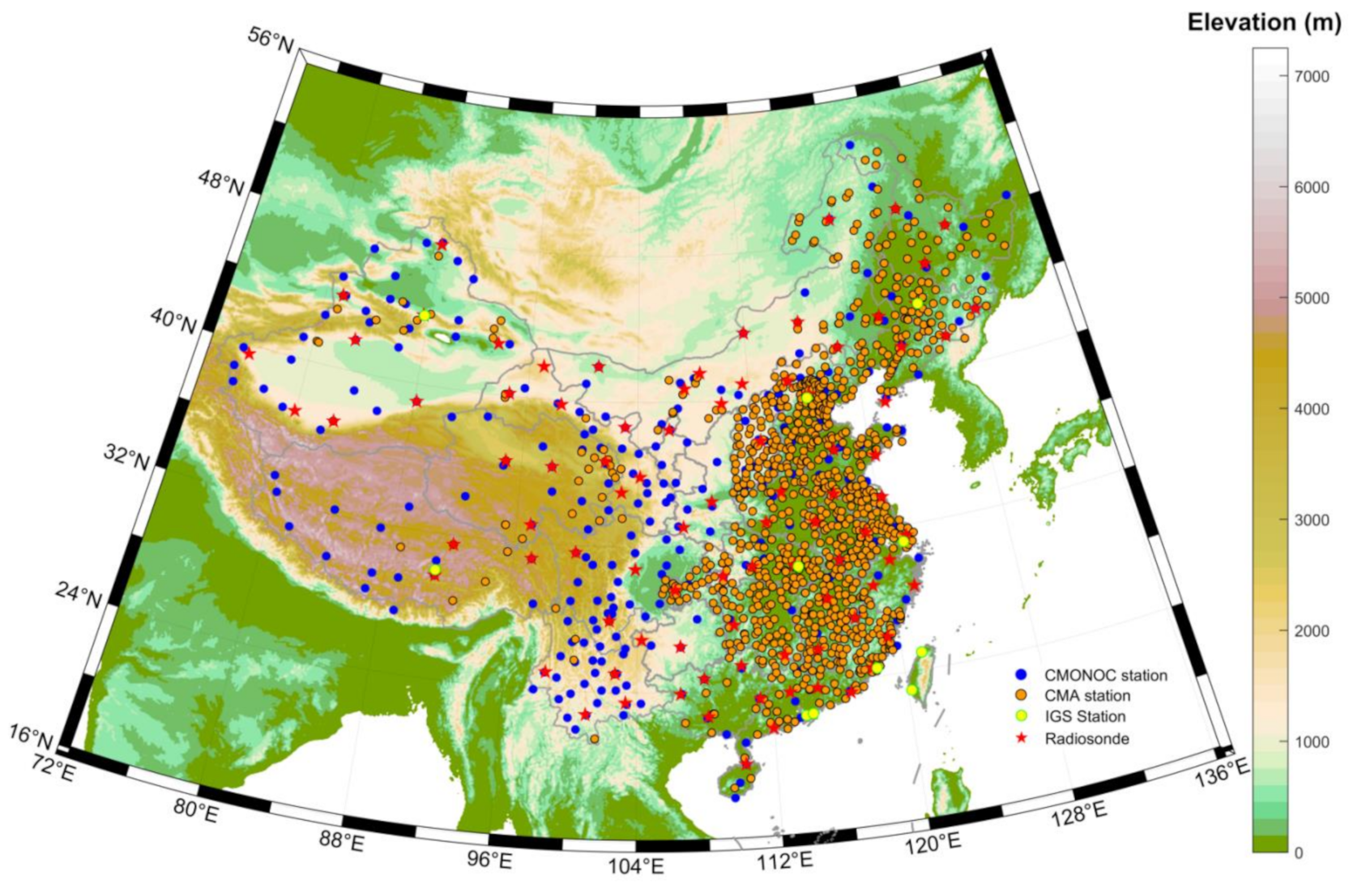
The research area is shown in
Figure 1 which covers the whole China land region. The hills in the south, the plains in the north, the deserts in the northwest, and the Qinghai-Tibet Plateau make up the main geographical landscapes of China. Complicated terrain makes water vapor variation pattern very complex. In this study, we use 11 International GNSS Service (IGS) stations, 1052 China Meteorological Administration (CMA) GNSS stations, and 254 Crustal Movement Observation Network of China (CMONOC) GNSS stations to modify the accuracy of the MODIS PWV in 2019. We use radiosonde data to assess the accuracy of GNSS PWV, and the detailed information can be found in
Appendix A.
2.2. PWV Data
The PWV data used in this study include the GNSS PWV and MODIS PWV. We use the GNSS PWV to calibrate the MODIS PWV. The GNSS PWV used in this study has two sources. One is provided by the Meteorological Observation Center of CMA [
21]. Another is to use a Precise Point Positioning (PPP) solution software which is developed by Yao Yibin’s group at Wuhan University to process the IGS and CMONOC GNSS observation. The strategy to obtain PPP-derived PWV can be found in Yao et al. [
22]. The temporal resolution of the CMA PWV used in this manuscript is 1 hour while PPP-derived PWV is 30 min. We use Radiosonde data to assess the accuracy of CMA PWV and PPP-derived PWV, and the results are presented in
Table 1 in terms of Bias, the standard deviation (STD), and the RMS. The method to obtain Radiosonde PWV and how to use Radiosonde PWV to assess the accuracy of GNSS PWV can be found in
Appendix A. All PWV have an accuracy within 2 mm which indicates that the GNSS PWV could be used to calibrate the MODIS PWV.
The MODIS PWV from MOD05_L2 includes Near Infrared (NIR) PWV and Infrared (IR) PWV. The NIR PWV has a spatial resolution of 1 km while the spatial resolution of the IR PWV is 5 km, and the NIR PWV has higher accuracy than the IR PWV [
23,
24]. We use the NIR PWV in this study. All available data within the research area in 2019 are collected and used. These data were acquired during 02:00–07:00 UTC daily. We remove the negative values and those in the top 0.5%. Only the NIR PWV on land under cloudless conditions is selected. The height information of the MODIS PWV is obtained from the Shuttle Radar Topography Mission Digital Elevation Model (STRM DEM) Version 4.1 data with a spatial resolution of 250 m [
25,
26]. The height system used in this study is the orthometric height, and the method of converting the ellipsoid height of the GNSS PWV to the orthometric height can be found in Li et al. [
27].
3. Methodology
Some scholars have done some studies in geoscience using those three machine learning methods, namely, BPNN, RF and GRNN, such as monitoring the variation of vegetation water content [
28] and estimating the weighted mean temperature [
29]. In this manuscript, BPNN, RF, and GRNN methods are used to calibrate the accuracy of MODIS PWV, and their performance is evaluated. At the same time, we use the MLR method for comparison.
3.1. BPNN
In machine learning, the BPNN is a widely used feed-forward neural network training algorithm, which was first proposed by Rumelhart et al. [
30,
31]. The BPNN analyzes the error information between each training result and the target result, and it continuously adjusts the threshold and weight to approximate the target result [
32].
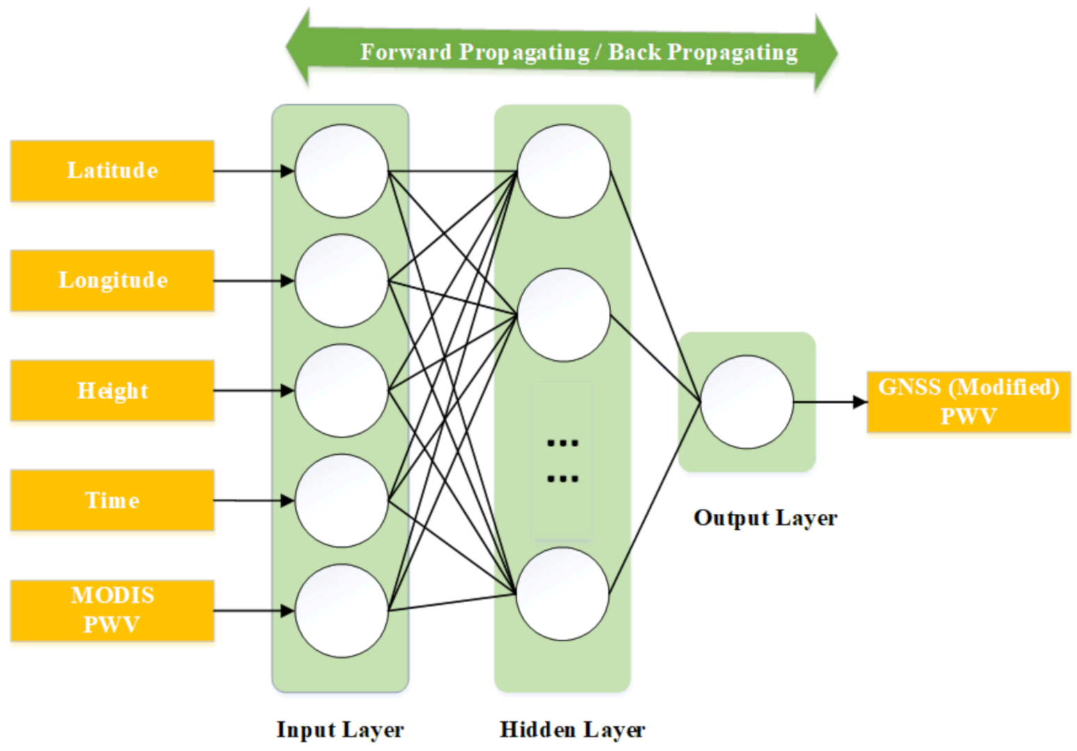
The BPNN includes three layers: the input layer, the hidden layer, and the output layer. The number of neurons in the input layer is equal to the dimension of each learning sample point. The number of neurons in the output layer is equal to the dimension of the output learning sample vector. The number of hidden layers and the number of neurons in each hidden layer are hyperparameters that need to be set at first. Almost every bounded continuous function can be approximated with an arbitrarily small error by a neural network with a single hidden layer [
33]. Therefore, we only use one hidden layer in this study.
The structure of the MODIS–GNSS PWV BPNN model is shown in
Figure 2. The input layer used in this study has five neurons corresponding to the longitude, latitude, elevation, observation time of a GNSS station, and the interpolated MODIS PWV at the GNSS station. In addition, there is only one neuron in the output layer corresponding to the GNSS PWV or the modified MODIS PWV.
When the BPNN is trained, it includes two processes: forward propagation and back propagation. In the forward propagation, signals from the input layer are transmitted to the output layer through the hidden layer. If there is a big gap between the result of the output layer and the target data, the back propagation is carried out to update the weight in the hidden layer. The training is not finished until the maximum number of iterations or the expected result is reached.
In the BPNN, each neuron in one layer is directly connected to the neurons of the subsequent layer with an activation function. In this study, we adopt the hyperbolic tangent function as the activation function between neurons in the input and hidden layers:
In addition, we adopt the linear function as the activation function between neurons in the hidden and output layers:
Then the final output of the BPNN can be written as
where
W2,1 and
W3,2 are weight matrices and
b1 and
b2 are bias matrices; these four matrices store the coefficients of the BPNN and should be optimized via back-propagation algorithm [
32],
X and
Y are respectively the input and output variables.
3.2. RF
The Random forest is an ensemble learning method that can be used for regression or classification. The RF constructs a large number of decision trees during training and then outputs the mode of the classes or the average prediction of the individual trees [
34,
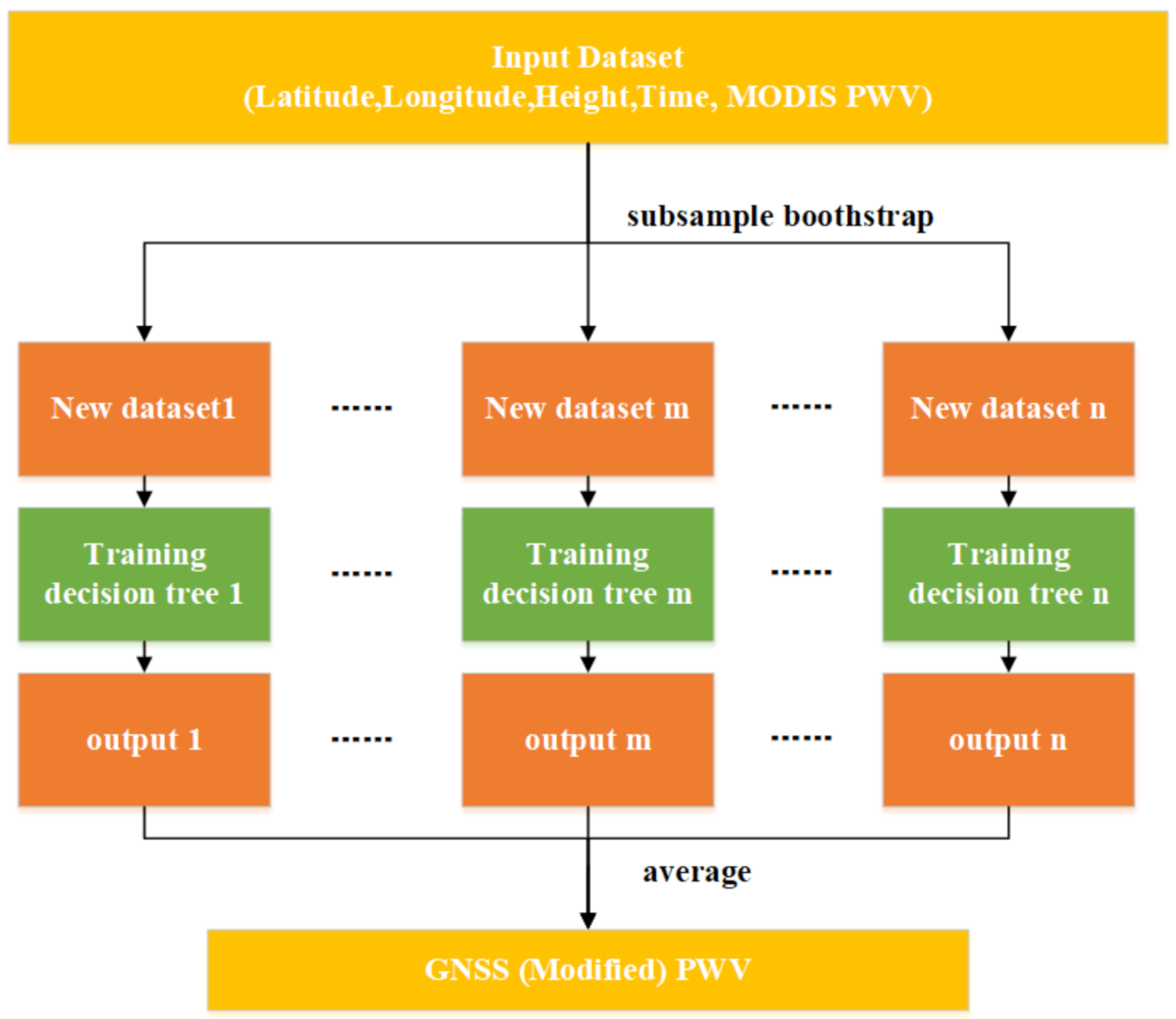
35]. The training method used in the random forest is called bootstrap aggregation. In other words, the RF uses a recursive partition method to generate many new datasets with same scale from the sample itself and then build models on each new dataset independently.
Figure 3 shows the structure of the MODIS–GNSS PWV RF calibrate model. The input data include latitude, longitude, height, observation time of a GNSS station, and the interpolated MODIS PWV at the GNSS station. The output data are the GNSS PWV or the modified MODIS PWV. The final model result is the average of all decision tree results.
where
X indicates the input variables,
Y is the final output of the RF,
Tb denotes the output of each regression tree, and
B is the number of trees.
For a single decision tree, it may overfit. The RF introduces randomness into each independent decision tree and takes the average of the results, which can effectively overcome the overfitting problem. For the RF, the number of decision trees has an important impact on the accuracy of the model and needs to be set. Generally, the number of decision trees is regarded as a hyperparameter and can be determined by the enumeration method.
In the regression problem, the random forest has the advantages of fast training speed and strong anti-interference ability. In the case of a large amount of missing data, the random forest can also achieve good results, but the random forest itself cannot give continuous output, so it cannot give predictions beyond the training range.
3.3. GRNN
The GRNN was proposed by Specht in 1991 [
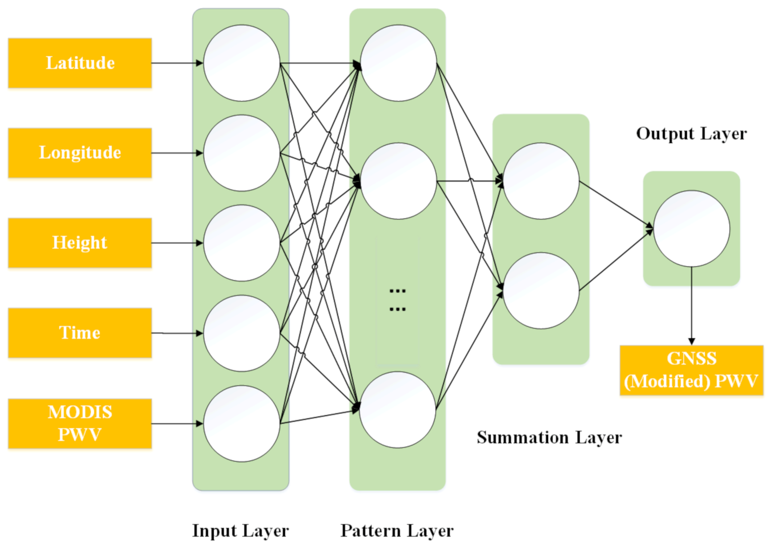
36]. The GRNN has a strong nonlinear mapping capability and flexible network structure. Moreover, it has high fault tolerance and robustness. The GRNN is suitable for solving nonlinear problems. The GRNN has a four-layer structure with an input layer, a pattern layer, a summation layer, and an output layer. The number of neurons in the input layer is equal to the dimension of the input learning sample vector.
Figure 4 shows the MODIS–GNSS PWV GRNN calibrate model. The input layer of the MODIS–GNSS PWV GRNN calibrate model has five neurons corresponding to the longitude, latitude, elevation, observation time of a GNSS station, and the interpolated MODIS PWV at the GNSS station. The number of neurons in the output layer is equal to the dimension of the output sample vector. There is only one neuron in the output layer in this experiment which is the GNSS PWV or modified MODIS PWV. The summation layer includes two types of summation neurons. They are used to compute the arithmetic summation and weighted summation of the outputs of all pattern layer neurons, respectively. The number of neurons in the pattern layer is equal to the number of learning samples. The transfer function of neurons in the pattern layer is
where
is the output of neuron
i in the pattern layer, which is an exponential function of the square of the Euclidean distance between the input variable,
the
i-th learning sample, and its corresponding testing sample
.
is called spread parameter (sp) and needs to be set at first. Large sp could make the estimation smooth while the small sp might make the results too close to learning samples (Specht, 1991).
3.4. 10-Fold Cross-Validation
The 10-fold cross-validation method is used to assess model accuracy in this study. The 10-fold cross-validation method randomly divides the dataset into 10 equal parts and selects one of them as the testing samples and nine as the training samples without duplication. After repeated 10 times, each part in the sample has been used as testing data once, and as training data nine times.
3.5. Multiple Linear Regression for Comparison
In this study, the MLR model is used for comparison. This is a common regression approach that models the relationship between input and output variables based on a linear assumption (Andrews, 1974). In this study, we built the MLR model using the following equation:
where t is the observation time of PWV data; lat and lon, respectively, represent the latitude and longitude, hgt is the height (m);
α0 is the intercept;
α1–α
5 are the regression coefficients for the input variables, derived using least-squares method, and every model is tested by 10-fold cross-validation method.
4. Model Construction and Performance
4.1. Formation of PWV Data Pairs
The above three machine learning methods are all used to modify the accuracy of the 2019 MODIS PWV in China land region with the GNSS PWV as the target. Annual and monthly models are constructed. At first, we need to match GNSS PWV and MODIS PWV both in spatial and temporal fields to form input-output pairs before establishing models. In the temporal filed, we take the time of the MODIS PWV as the time tag. When the difference between the GNSS PWV time and MODIS PWV time is within 30 min, they are treated at the same time. In the spatial filed, we first use the spherical cap harmonic (SCH) function to fit the MOIDS PWV and then use the function to interpolate it to the GNSS station to obtain the MODIS PWV at a GNSS station. The SCH function order used to fit MODIS PWV is 5 since it has the smallest fitting RMS compared to corresponding GNSS PWV. Because the area covered by the MODIS PWV data are inconsistent over time, the pole of the spherical cap is chosen at the center of the MODIS PWV data. Finally, we obtain 208,010 MODIS–GNSS pairs in 2019.
To remove the outliers which will affect the performance of machine learning methods, we compute the Bias and STD from the differences based on the entire dataset and then use Bias ± 3 STD as the threshold to remove any data pair whose difference is larger than the threshold. After that, 203,820 MODIS–GNSS pairs remain, and we can train models based on these data pairs. The statistics of the remaining MODIS–GNSS pairs in terms of Bias, STD, RMS, and correlation coefficient R are −2.3 mm, 5.4 mm, 5.9 mm and 0.96, respectively.
4.2. Determine Hyperparameters
The number of decision trees in the RF, the number of neurons in the hidden layer for the BPNN, and the spread parameter for the GRNN are hyperparameters that need to be set. Determining the hyperparameters requires comprehensive consideration of the cross-validation accuracy, the fitting accuracy, and the computational efficiency. We use the enumeration method to determine the model hyperparameter values. All models are assessed with 10-fold cross-validation method and compared with the GNSS PWV. For the RF, we set the number of decision trees between 5 and 105 at a step of 5. As the acceleration in computation speed, the number of neurons in the hidden layer of the BPNN is usually set to the integer power of 2 (Hornik et al., 1989). Therefore, we set the neuron number as 2, 4, 8, 16, 32, 64, 128, and 256. For the GRNN, a series of optional spread parameter values between 0.01 and 0.2 at a step of 0.01 is set. In addition, to make the cross-validation accuracy as high as possible, the superparameter should also make the cross-validation accuracy and the fitting accuracy comparable. The computational efficiency should also be taken into account. The determined optimal hyperparameters are given in
Table 2 and
Table 3, respectively, for the annual and monthly models.
4.3. Model Performance at Annual Timescale
At first, we establish the annual MODIS–GNSS PWV models with the three machine learning methods. We use the whole year data in 2019 to train the model and obtain one annual model for each method. The modified accuracy is obtained by the 10-fold cross-validation and listed in
Table 2, as well as the optimal hyperparameter values, and the MLR method is used for comparison.
Table 2.
Annual MODIS–GNSS PWV model results compared to GNSS PWV.
Table 2.
Annual MODIS–GNSS PWV model results compared to GNSS PWV.
| | Accuracy | Hyperparameter | Bias (mm) | STD (mm) | RMS (mm) | R |
|---|
| | Original | - | −2.4 | 5.3 | 5.8 | 0.95 |
| GRNN | Modified | 0.05 | 0.1 | 3.9 | 3.9 | 0.97 |
| Fitting | 0.05 | −0.1 | 3.6 | 3.6 | 0.98 |
| RF | Modified | 70 | 0.0 | 3.3 | 3.3 | 0.98 |
| Fitting | 70 | 0.0 | 2.3 | 2.3 | 0.99 |
| BPNN | Modified | 256 | 0.0 | 4.1 | 4.1 | 0.97 |
| Fitting | 256 | 0.0 | 4.1 | 4.1 | 0.97 |
| MLR | Modified | − | 0.0 | 5.0 | 5.0 | 0.96 |
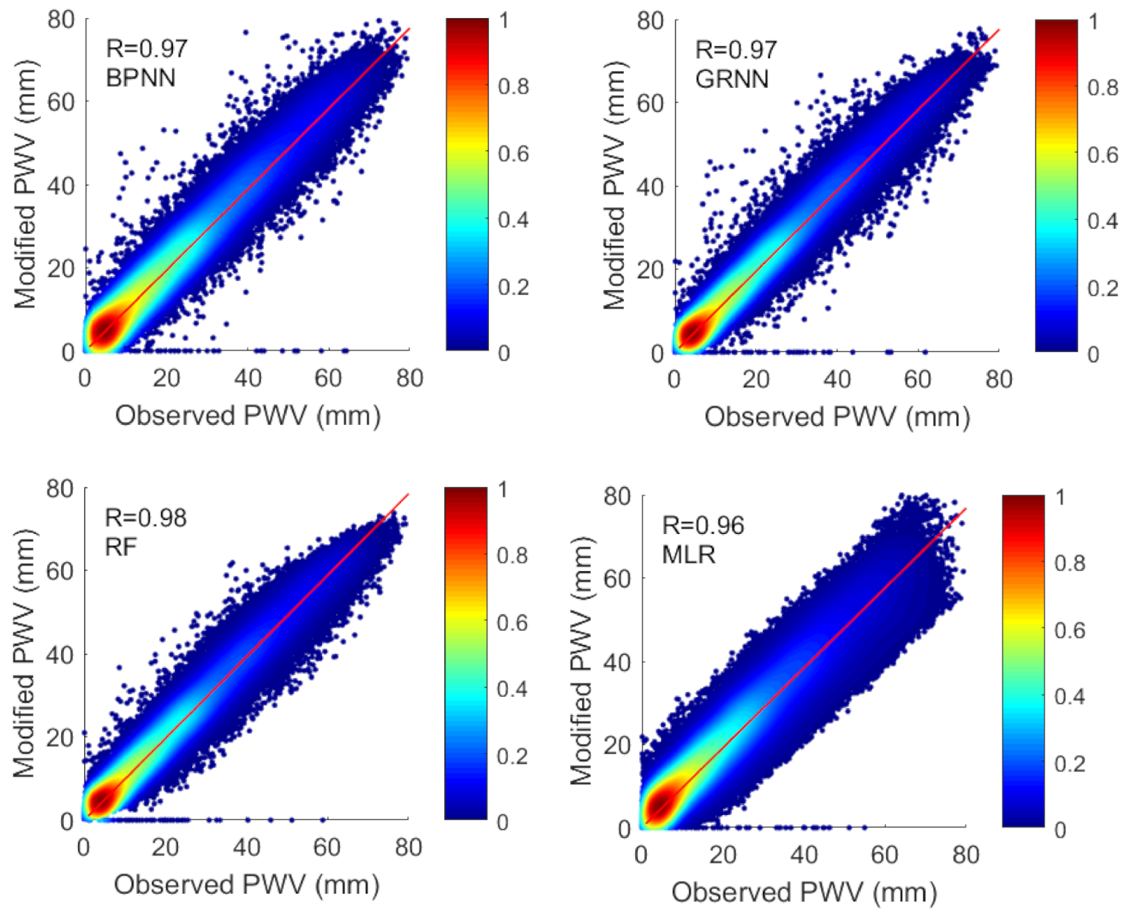
It is seen that the statistics with the modified and fitting PWVs are comparable, which indicates that all the trained models are not overfitting. The RMSs are reduced from original 5.8 mm to 3.9, 3.3, 4.1, and 5.0 mm after the training by the GRNN, RF, BPNN, and MLR, respectively, with improvements of 33.0%, 43.2%, 29.3%, and 13.8%. The correlation coefficient R is increased from 0.95 to 0.97, 0.98, 0.97, and 09.6 for the GRNN, RF, BPNN, and MLR, respectively. It can be seen that the RF has the best performance in training MODIS–GNSS PWV model in annual scale, and all three machine learning methods perform better than MLR method. This is because the machine learning methods are better to simulate the complex nonlinear relationship and the hidden features within the datasets [
28].
The scatter plots between the modified MODIS PWV and GNSS PWV obtained by 10-fold cross-validation are shown in
Figure 5. It is seen that the modified MODIS PWV and GNSS PWV have a highly linear correlation.
4.4. Model Performance at Monthly Timescale
The accuracy of the annual MODIS–GNSS PWV models is demonstrated to better than that of the original MODIS PWV. It would be further improved if variation patterns in the PWVs can be considered. As such, we use the whole month data to train the model, resulting in 12 monthly models in 2019 for each method.
Table 3.
Monthly MODIS–GNSS PWV model results compared to GNSS PWV.
Table 3.
Monthly MODIS–GNSS PWV model results compared to GNSS PWV.
| Month | Original Accuracy | Methods | | Modified Accuracy | Fitting Accuracy |
|---|
| Hyperparameter | Bias | STD | RMS | R | Bias | STD | RMS | R |
|---|
| 201901 | Bias | −1.8 | GRNN | 0.05 | 0.0 | 1.7 | 1.7 | 0.98 | 0.0 | 1.1 | 1.1 | 0.99 |
| STD | 4.0 | BPNN | 128 | 0.0 | 1.8 | 1.8 | 0.98 | 0.0 | 1.5 | 1.5 | 0.99 |
| RMS | 4.4 | RF | 40 | 0.0 | 2.0 | 2.0 | 0.98 | 0.0 | 1.3 | 1.3 | 0.99 |
| R | 0.91 | MLR | - | 0.0 | 3.5 | 3.5 | 0.92 | - | - | - | - |
| 201902 | Bias | −1.4 | GRNN | 0.06 | 0.0 | 1.7 | 1.7 | 0.98 | 0.0 | 1.2 | 1.2 | 0.99 |
| STD | 4.2 | BPNN | 128 | 0.0 | 1.9 | 1.9 | 0.98 | 0.0 | 1.5 | 1.5 | 0.99 |
| RMS | 4.4 | RF | 60 | 0.0 | 1.9 | 1.9 | 0.98 | 0.0 | 1.3 | 1.3 | 0.99 |
| R | 0.9 | MLR | - | 0.0 | 3.5 | 3.5 | 0.92 | - | - | - | - |
| 201903 | Bias | −1.0 | GRNN | 0.05 | 0.0 | 2.2 | 2.2 | 0.98 | 0.0 | 1.3 | 1.3 | 0.99 |
| STD | 4.0 | BPNN | 128 | 0.0 | 2.4 | 2.4 | 0.97 | 0.0 | 2.1 | 2.1 | 0.98 |
| RMS | 4.2 | RF | 85 | 0.0 | 2.4 | 2.4 | 0.97 | 0.0 | 1.6 | 1.6 | 0.99 |
| R | 0.93 | MLR | - | 0.0 | 3.8 | 3.8 | 0.93 | - | - | - | - |
| 201904 | Bias | −1.5 | GRNN | 0.06 | 0.0 | 2.9 | 2.9 | 0.97 | 0.0 | 1.8 | 1.8 | 0.99 |
| STD | 4.9 | BPNN | 128 | 0.0 | 3.1 | 3.1 | 0.97 | 0.0 | 2.6 | 2.6 | 0.98 |
| RMS | 5.1 | RF | 50 | 0.0 | 3.0 | 3.0 | 0.97 | 0.0 | 2.1 | 2.1 | 0.99 |
| R | 0.93 | MLR | - | 0.0 | 4.6 | 4.6 | 0.93 | - | - | - | - |
| 201905 | Bias | −1.6 | GRNN | 0.07 | 0.1 | 3.0 | 3.0 | 0.98 | 0.0 | 2.0 | 2.0 | 0.99 |
| STD | 4.7 | BPNN | 128 | 0.0 | 3.1 | 3.1 | 0.97 | 0.0 | 2.5 | 2.5 | 0.98 |
| RMS | 5.0 | RF | 65 | 0.0 | 3.2 | 3.2 | 0.97 | 0.0 | 2.2 | 2.2 | 0.99 |
| R | 0.94 | MLR | - | 0.0 | 4.4 | 4.4 | 0.94 | - | - | - | - |
| 201906 | Bias | −2.6 | GRNN | 0.06 | 0.0 | 3.4 | 3.4 | 0.98 | 0.0 | 2.4 | 2.4 | 1.00 |
| STD | 5.8 | BPNN | 128 | 0.0 | 3.7 | 3.7 | 0.97 | 0.0 | 3.3 | 3.3 | 0.98 |
| RMS | 6.4 | RF | 50 | 0.0 | 3.7 | 3.7 | 0.97 | 0.0 | 2.5 | 2.5 | 0.99 |
| R | 0.93 | MLR | - | 0.0 | 5.7 | 5.7 | 0.94 | - | - | - | - |
| 201907 | Bias | −4.2 | GRNN | 0.06 | 0.0 | 3.5 | 3.5 | 0.97 | 0.0 | 2.7 | 2.7 | 0.99 |
| STD | 6.8 | BPNN | 128 | 0.0 | 4.0 | 4.0 | 0.97 | 0.0 | 3.6 | 3.6 | 0.97 |
| RMS | 8.0 | RF | 80 | 0.0 | 3.8 | 3.8 | 0.97 | 0.0 | 2.6 | 2.6 | 0.99 |
| R | 0.91 | MLR | - | 0.0 | 6.1 | 6.1 | 0.92 | - | - | - | - |
| 201908 | Bias | −3.8 | GRNN | 0.06 | 0.0 | 3.6 | 3.6 | 0.97 | 0.0 | 2.8 | 2.8 | 0.99 |
| STD | 6.6 | BPNN | 128 | 0.0 | 4.2 | 4.2 | 0.96 | 0.0 | 3.8 | 3.8 | 0.97 |
| RMS | 7.6 | RF | 95 | 0.0 | 3.9 | 3.9 | 0.97 | 0.0 | 2.6 | 2.6 | 0.99 |
| R | 0.91 | MLR | - | 0.0 | 6.4 | 6.4 | 0.91 | - | - | - | - |
| 201909 | Bias | −3.4 | GRNN | 0.05 | 0.0 | 2.8 | 2.8 | 0.98 | 0.0 | 1.9 | 1.9 | 0.99 |
| STD | 5.6 | BPNN | 128 | 0.0 | 3.3 | 3.3 | 0.97 | 0.0 | 3.0 | 3.0 | 0.98 |
| RMS | 6.5 | RF | 90 | 0.0 | 3.2 | 3.2 | 0.97 | 0.0 | 2.1 | 2.1 | 0.99 |
| R | 0.93 | MLR | - | 0.0 | 5.2 | 5.2 | 0.93 | - | - | - | - |
| 201910 | Bias | −2.2 | GRNN | 0.05 | 0.0 | 2.3 | 2.3 | 0.98 | 0.0 | 1.6 | 1.6 | 1.00 |
| STD | 5.3 | BPNN | 128 | 0.0 | 2.8 | 2.8 | 0.98 | 0.0 | 2.5 | 2.5 | 0.98 |
| RMS | 5.7 | RF | 75 | 0.0 | 2.6 | 2.6 | 0.98 | 0.0 | 1.8 | 1.8 | 0.99 |
| R | 0.93 | MLR | - | 0.0 | 4.8 | 4.8 | 0.93 | - | - | - | - |
| 201911 | Bias | −2.1 | GRNN | 0.05 | 0.0 | 1.8 | 1.8 | 0.98 | 0.0 | 1.2 | 1.2 | 0.99 |
| STD | 4.2 | BPNN | 128 | 0.0 | 2.1 | 2.1 | 0.97 | 0.0 | 1.8 | 1.8 | 0.98 |
| RMS | 4.7 | RF | 55 | 0.0 | 2.0 | 2.0 | 0.97 | 0.0 | 1.4 | 1.4 | 0.99 |
| R | 0.91 | MLR | - | 0.0 | 3.5 | 3.5 | 0.92 | - | - | - | - |
| 201912 | Bias | −1.4 | GRNN | 0.05 | 0.0 | 1.6 | 1.6 | 0.98 | 0.0 | 1.2 | 1.2 | 0.99 |
| STD | 3.4 | BPNN | 128 | 0.0 | 1.8 | 1.8 | 0.97 | 0.0 | 1.6 | 1.6 | 0.98 |
| RMS | 3.7 | RF | 55 | 0.0 | 1.7 | 1.7 | 0.98 | 0.0 | 1.2 | 1.2 | 0.99 |
| R | 0.92 | MLR | − | 0.0 | 3.0 | 3.0 | 0.92 | − | − | − | − |
Table 3 presents the statistics of all the monthly MODIS–GNSS PWV models trained by the three machine learning methods and the MLR method. The monthly RMS of the original MODIS PWV in China region is typically about 4–6 mm. However, it varies from month to month, and the worst is 8.0 mm in July. Again, the comparable statistics with the modified and fitting PWVs indicate that all monthly MODIS–GNSS models are not overfitting.
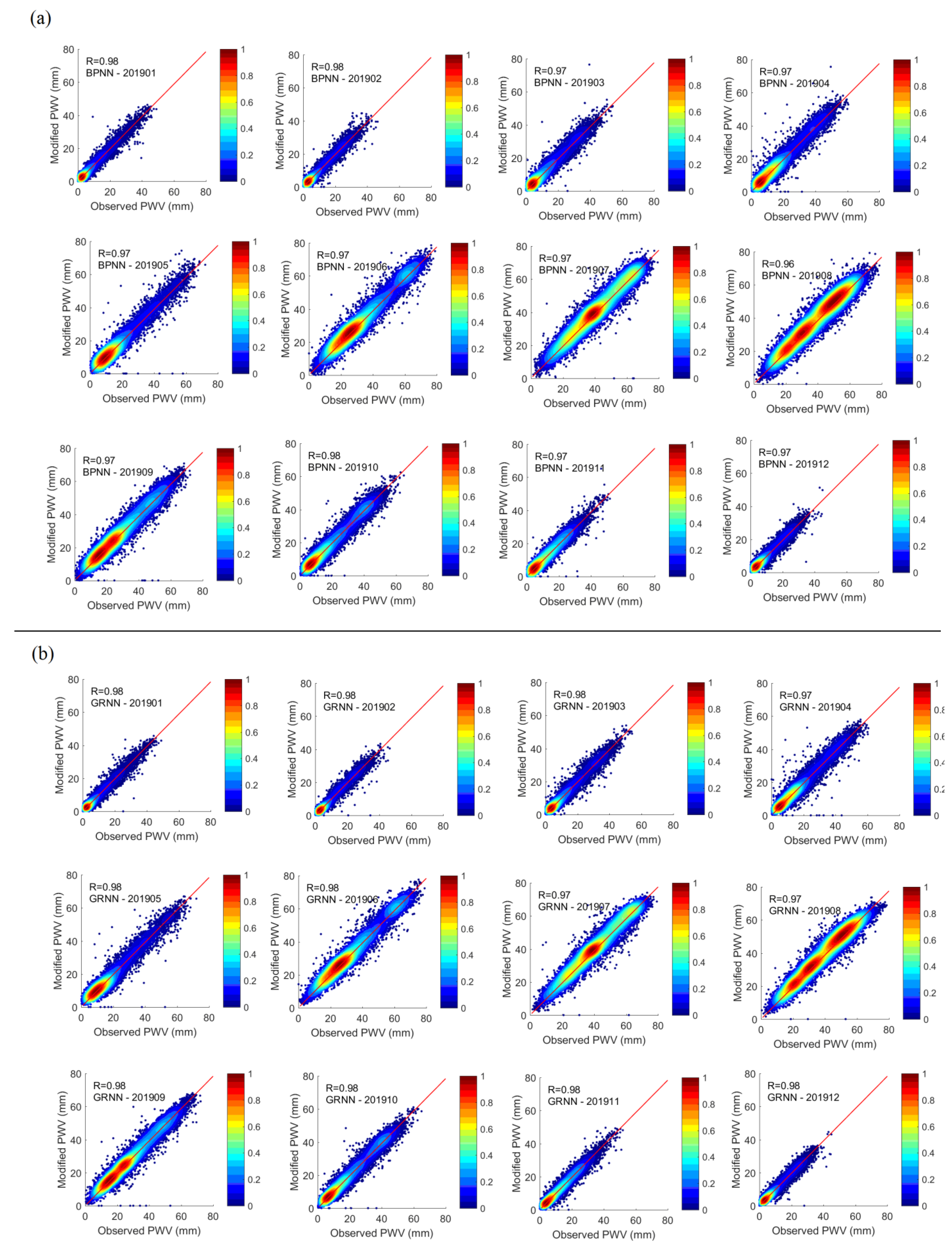
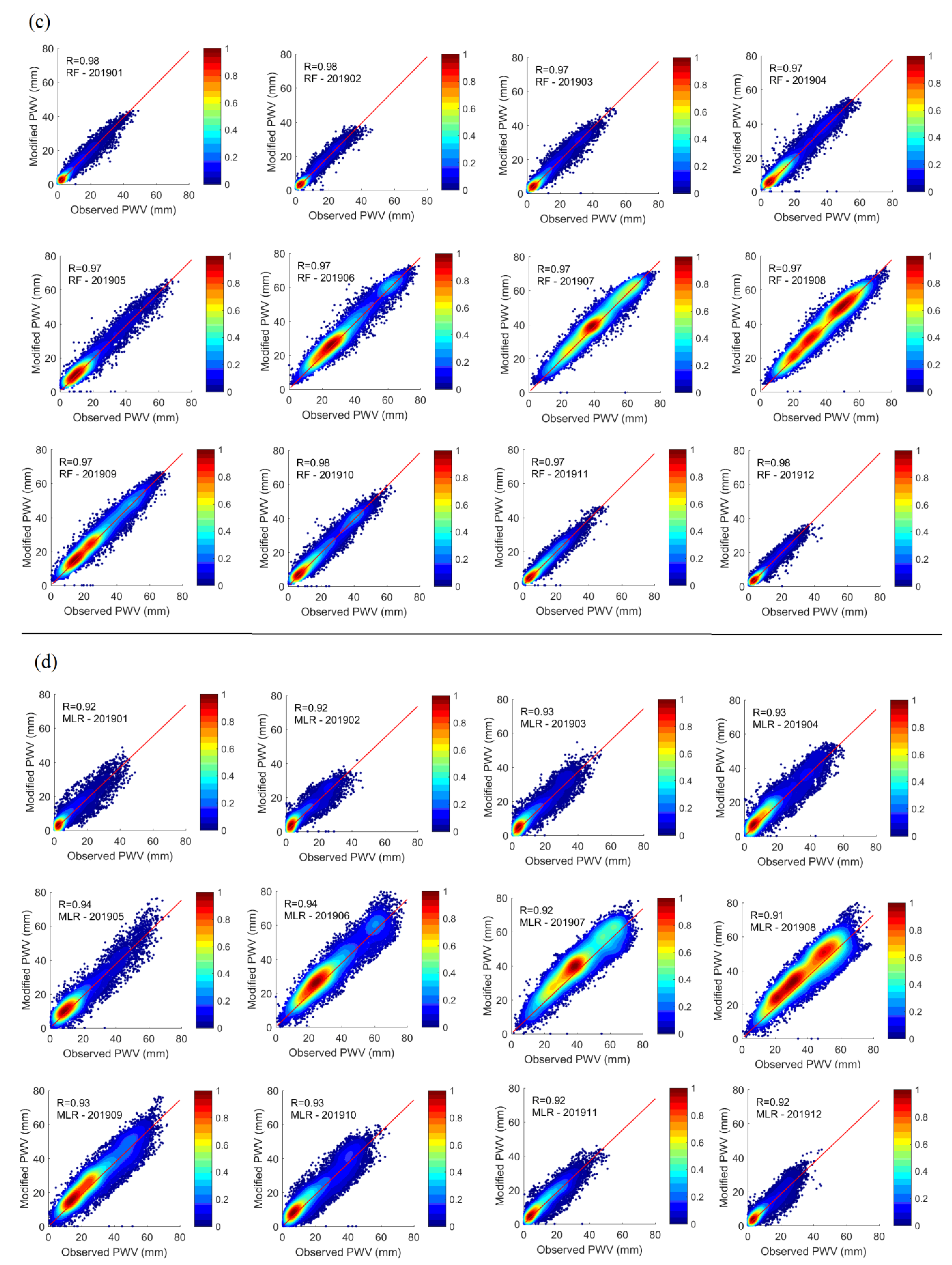
As shown in
Figure 6, the modified MODIS PWV has a strong linear correlation with the GNSS PWV. For the RF, the smallest RMS reductions are 55.6% (January), 36.1% (May), 41.4% (June), and 51.4% (September), respectively, for the winter, spring, summer and autumn seasons. For the BPNN, they are 56.0% (February), 38.0% (May), 41.3% (June), and 49.9% (September), respectively. For the GRNN, the smallest RMS reductions for the four seasons are 60.4% (February), 40.3% (May), 47.1% (June), and 57.1% (September), respectively. The accuracy improvements, in terms of the RMS, of the monthly MODIS–GNSS models trained by the three methods are all greater than those of the corresponding annual models. In addition, all three machine learning methods achieve better performance than the MLR method in every month in 2019 since the RMSs of MLR method are greater than that of machine learning methods.
The average RMS values of the methods are 2.9 mm (BPNN), 2.8 mm (RF), 2.5 mm (GRNN), and 4.6 mm (MLR). The GRNN presents the best performance in modeling MODIS–GNSS PWV data pairs at the monthly scale.
The difference between the RMS of the annual model and the mean RMS of monthly models are 1.2 mm (BPNN), 0.5 mm (RF), and 1.4 mm (GRNN). For the RF, because it randomly generates some decision trees and takes the average of those decision tree results as the final result, it could suppress the influence caused by the variety of different samples. Therefore, the RF has the smallest RMS difference between the annual model and the monthly model. For the GRNN, the modeling directly depends on the original training samples. Therefore, the variation pattern in the training sample would affect the accuracy of GRNN result. When a large sample is divided into several sub-samples each having smaller internal differences, the GRNN model performance can be further improved. The training time of the BPNN model is significantly increased compared with the RF and GRNN, and the BPNN training is prone to fall into the local optimum trap during the parameter fitting. Therefore, the BPNN is inferior to the RF and GRNN in both training efficiency and accuracy. If there is an obvious variation pattern in training samples, the RF will achieve a better performance than the GRNN since RF achieve the best performance among those three machine learning methods. However, dividing such training samples into smaller sub-samples according to the variation pattern can improve the performance of machine learning methods, especially the performance of the GRNN.
5. Accuracy Analysis
Since all machine learning methods achieve the better performance at a monthly timescale than at the annual scale, we only discuss the spatial and temporal performance of the monthly models in the following.
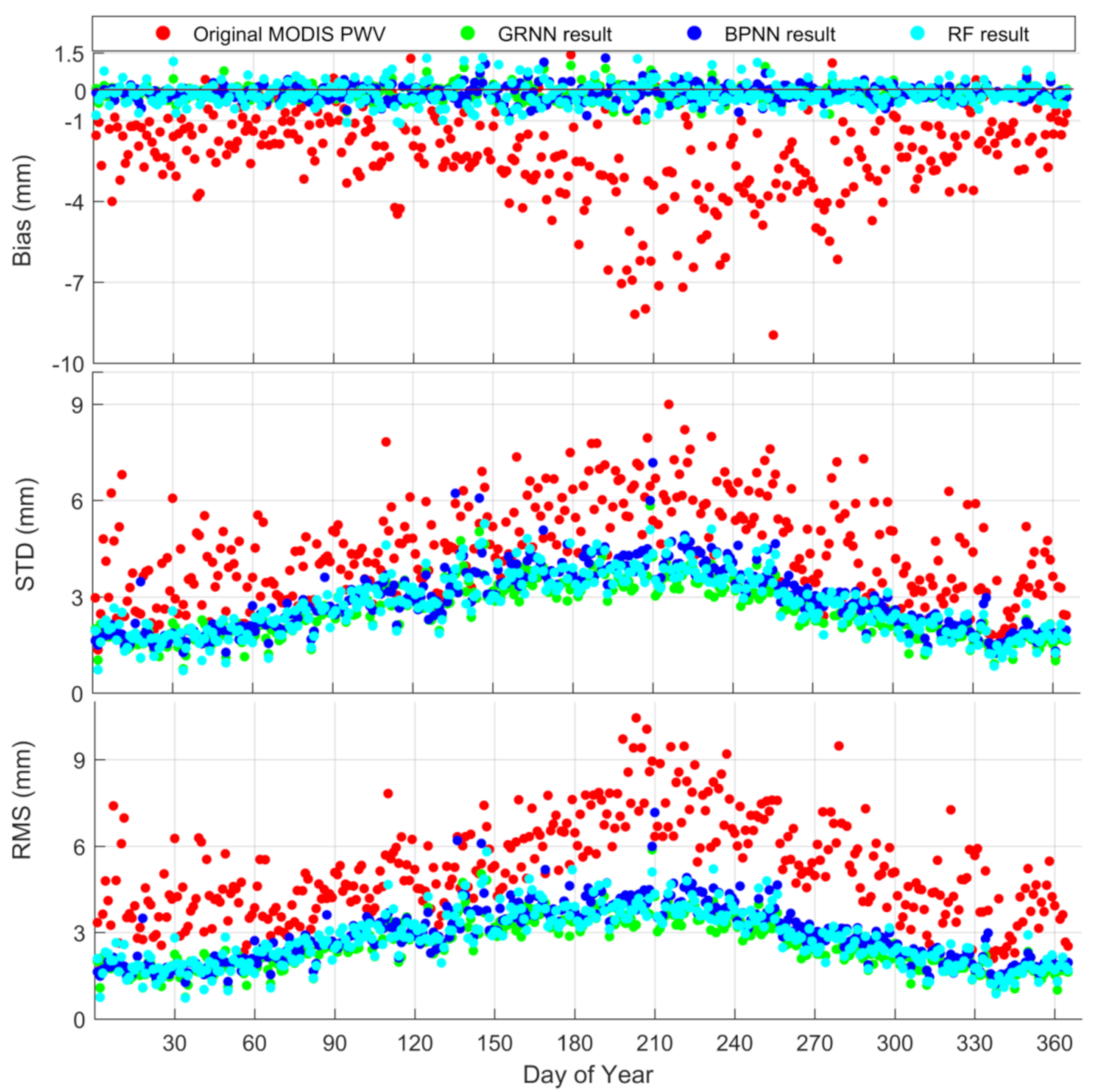
Figure 7 shows the daily Bias, STD, and RMS values in 2019. It is seen that these daily values vary with some patterns in 2019. For the STD and RMS, they increase from day 1 to day 210 and then decrease. Applying the three machine learning methods has effectively flattened the curves. The system difference between the original MODIS PWV and GNSS PWV is essentially eliminated, since all the bias values between the modified MODIS PWV and GNSS PWV are close to 0. The day-to-day STD and RMS variations are weakened after the modeling. In addition, as it can be seen in
Figure 7, the GRNN models have the smallest STD and RMS, and the BPNN has the largest RMS, which indicates that the GRNN achieves the best performance among the three machine learning methods for the monthly modeling.
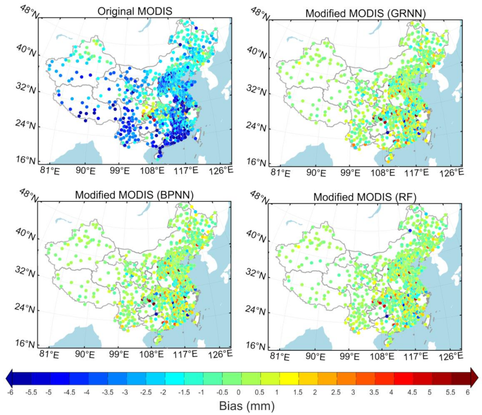
Figure 8 shows the biases between the original/modified MODIS PWV and GNSS PWV at the GNSS sites. As it can be seen from
Figure 8, the biases are reduced in all regions for all three machine learning methods, which indicates that they can effectively eliminate the system deviation in any area. However, it is shown in
Figure 8 that the bias of a very small part of the stations (e.g., along the Yangtze River, south-eastern China, and Shanxi province) is relatively large after modifying. In this subset of stations, data are available for only a small number of dates in 2019. The bias obtained from fewer data could not well reflect the real effect of the model.
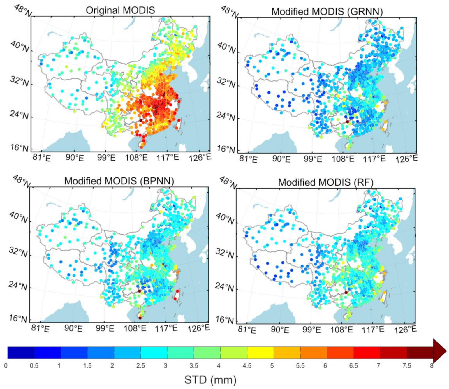
Figure 9 shows the spatial distribution of STDs of the differences between the original/modified MODIS PWV and GNSS PWV. The STD with respect to the original MODIS PWV is larger in the east of the Heihe-Tengchong line while smaller in the west of the line. The spatial distribution of STDs is much more even after the modeling by the three machine learning methods. It can be seen that the GRNN and RF achieve better performance than the BPNN, especially in Taiwan province. In most areas, the differences in STDs from the three models are only minor. It may be noted that the STDs with the GRNN method in the north of China are smaller than those with the BPNN and RF methods.
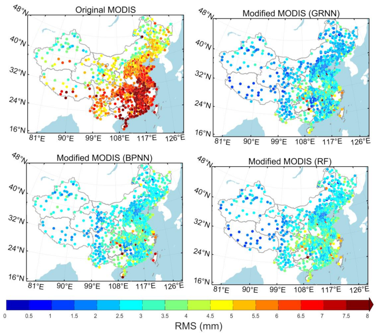
Figure 10 shows the RMS spatial distribution, and its variation pattern is similar to that of the STDs. If the bias is close to zero, the difference between STD and RMS will be small. However, there were differences in RMS and STD in some regions (e.g., along the Yangtze River, south-eastern China, and Shanxi province) compared with
Figure 9 and
Figure 10, which was caused by the abnormal bias. In addition, the reduction of STD and RMS is relatively small while the bias is close to zero after modifying at two stations in Taiwan and one station in Hainan which is located at the edge of the study area. This shows that the modifying effect of the model may be limited in the marginal areas.
From the above results, it may be concluded that the GRNN models achieve the best performance among the three methods at monthly timescales for modifying 2019 MODIS PWV data in the China land region. The spatial distributions of STD and RMS values are similar to each other for the three machine learning methods. Both the spatial and temporal variation patterns are weakened through the three machine learning methods.
6. Conclusions
Since the accuracy of the MODIS PWV in China land region is poor compared to that in the U.S., we try to use different machine learning methods to modify the accuracy of MODIS PWV and evaluate the performance of different methods and modeling timescales. The GRNN, BPNN, and RF methods have been applied to the datasets in 2019 at annual and monthly timescale, and we use the MLR method for comparison. The RMSs of those methods at the annual timescale are 4.1 mm (BPNN), 3.3 mm (RF), 3.9 mm (GRNN), and 5.0 mm (MLR), and the average RMS values of the monthly modified MODIS PWV are 2.9, 2.8, 2.5, and 4.6 mm, respectively with the BPNN, RF, GRNN, and MLR methods. This indicates that the machine learning methods perform better than the traditional linear method, and GRNN method is the best in terms of the RMS for the given datasets at the monthly timescale while RF achieves the best performance at the annual timescale. The results also show that, when the training sample has an obvious variation pattern, the RF achieves the best performance since the RF achieves the best performance among those three machine learning methods at the annual timescale. On the other hand, dividing such sample into several sub-samples each having higher internal consistency could further enhance the performance of the machine learning methods, especially for the GRNN, since the model performance at monthly scale is better than that of annual scale, and the GRNN has the largest RMS difference between the two timescales among those three machine learning methods. Using GNSS PWV to modify the accuracy of MODIS PWV could enhance hydrological analysis in several developing countries where the availability of meteorological stations is limited.
Author Contributions
Conceptualization, Z.X. and X.S.; methodology, Z.X.; validation, Z.X.; formal analysis, Z.X. and J.S.; investigation, Z.X.; resources, X.S. and X.W.; data curation, Z.X.; writing—original draft preparation, Z.X.; writing—review and editing, J.S.; visualization, Z.X.; supervision, Z.X.; project administration, X.S.; funding acquisition, X.S. All authors have read and agreed to the published version of the manuscript.
Funding
This work was jointly supported by National key research and development program of China (2018YFC1506606) and Key project of basic scientific research operating expenses of Chinese Academy of Meteorological Sciences (2019Z003).
Institutional Review Board Statement
Not applicable.
Informed Consent Statement
Not applicable.
Data Availability Statement
GNSS data from China Meteorological Administration (CMA) can be accessed from
https://data.cma.cn/en/ (accessed on 25 April 2021), and GNSS data from the Crustal Movement Observation Network of China (CMONOC) is available through China Earthquake Administration. MODIS data used in this study is provided by NASA from the website at
https://ladsweb.modaps.eosdis.nasa.gov/search/ (accessed on 25 April 2021). The reanalysis data, ERA5 products, is accessed from ECMWF at
https://www.ecmwf.int/ (accessed on 25 April 2021).
Acknowledgments
Thanks to the help from Zhang Bao, Sun Zhangyu, Gong Xuewen at School of Geomatics, Wuhan University, and Zhao Tingting at No. 2 Middle School, Daoxian County, Hunan Province.
Conflicts of Interest
The authors declare no conflict of interest.
Appendix A. Radiosonde PWV Calculation Method
Radiosonde PWV can be obtained by Formulas (A1)–(A5).
where
is the water vapor pressure at each grid point in Pascal,
K/Pa, k
2 = 3.7310
−3 K
2/Pa, h the layer height in m.
where RH is the relative humidity. P
s is the saturated water vapor pressure which is related to the temperature and can be calculated by the Wexler formula [
37,
38].
The relationship between ZWD and PWV is shown as Formula (A3):
where
is a dimensionless conversion factor, and it is calculated by Equation (A4):
where
is the density of water,
the water vapor ratio constant,
,
, and
is the weighted average temperature computed with the method by Yao et al. [
39].
We use radiosonde data to assess the accuracy of the GNSS PWV. The radiosonde data is derived from the Integrated Global Radiosonde Archive Version 2 (IGRA2) dataset, whose distribution is shown in
Figure 1. Since the Radiosonde data is only released at 0:00 UTC and 12:00 UTC, the accuracy assessment of GNSS PWV is limited to these two time points. If the distance between the GNSS station and the radiosonde station within 60 km in the horizontal direction and the height difference less than 500 m, we use that Radiosonde PWV to assess the accuracy of the GNSS PWV. In addition, there are 89 radiosonde stations used to assess the accuracy of GNSS PWV.
We used the empirical formula (A5) to reduce the PWV value from a radiosonde station at height h
2 to that at a GNSS station at height h
1. All height belongs to the orthometric height system.
where PWV
h1 and PWV
h2 are the PWV values corresponding to the heights of h
1 and h
2, respectively.
References
- King, M.D.; Kaufman, Y.J.; Menzel, W.P.; Tanre, D. Remote sensing of cloud, aerosol, and water vapor properties from the moderate resolution imaging spectrometer (MODIS). IEEE Trans. Geosci. Remote Sens. 1992, 30, 2–27. [Google Scholar] [CrossRef] [Green Version]
- Nikiforov, A.Y.; Sarani, A.; Leys, C. The influence of water vapor content on electrical and spectral properties of an atmospheric pressure plasma jet. Plasma Sources Sci. Technol. 2011, 20, 015014. [Google Scholar] [CrossRef]
- Li, X.; Zus, F.; Lu, C.; Dick, G.; Ning, T.; Ge, M.; Wickert, J.; Schuh, H. Retrieving of atmospheric parameters from multi-GNSS in real time: Validation with water vapor radiometer and numerical weather model. J. Geophys. Res. Atmos. 2015, 120, 7189–7204. [Google Scholar] [CrossRef] [Green Version]
- Zhang, B.; Yao, Y.; Xin, L.; Xu, X. Precipitable water vapor fusion: An approach based on spherical cap harmonic analysis and Helmert variance component estimation. J. Geod. 2019, 93, 2605–2620. [Google Scholar] [CrossRef]
- Xiong, Z.; Sang, J.; Sun, X.; Zhang, B.; Li, J. Comparisons of Performance Using Data Assimilation and Data Fusion Approaches in Acquiring Precipitable Water Vapor: A Case Study of a Western United States of America Area. Water 2020, 12, 2943. [Google Scholar] [CrossRef]
- Liu, H.; Tang, S.; Zhang, S.; Hu, J. Evaluation of MODIS water vapour products over China using radiosonde data. Int. J. Remote Sens. 2015, 36, 680–690. [Google Scholar] [CrossRef]
- Gui, K.; Che, H.; Chen, Q.; Zeng, Z.; Liu, H.; Wang, Y.; Zheng, Y.; Sun, T.; Liao, T.; Wang, H.; et al. Evaluation of radiosonde, MODIS-NIR-Clear, and AERONET precipitable water vapor using IGS ground-based GPS measurements over China. Atmos. Res. 2017, 197, 461–473. [Google Scholar] [CrossRef]
- Li, Z. Production of Regional 1 km× 1 km Water Vapor Fields through the Integration of GPS and MODIS Data. In Proceedings of the 17th International Technical Meeting of the Satellite Division of ehe Institute of Navigation (ION GNSS 2004), Long Beach, CA, USA, 21–24 September 2014; pp. 2396–2403. [Google Scholar]
- Bevis, M.; Businger, S.; Herring, T.A.; Rocken, C.; Anthes, R.A.; Ware, R.H. GPS meteorology: Remote sensing of atmospheric water vapor using the Global Positioning System. J. Geophys. Res. Atmos. 1992, 97, 15787–15801. [Google Scholar] [CrossRef]
- Bevis, M.; Businger, S.; Chiswell, S.; Herring, T.A.; Anthes, R.A.; Rocken, C.; Ware, R.H. GPS meteorology: Mapping zenith wet delays onto precipitable water. J. Appl. Meteorol. 1994, 33, 379–386. [Google Scholar] [CrossRef]
- Yao, Y.; Shan, L.; Zhao, Q. Establishing a method of short-term rainfall forecasting based on GNSS-derived PWV and its application. Sci. Rep. 2017, 7, 12465. [Google Scholar] [CrossRef]
- Bock, O.; Nuret, M. Verification of NWP model analyses and radiosonde humidity data with GPS precipitable water vapor estimates during AMMA. Weather Forecast. 2009, 24, 1085–1101. [Google Scholar] [CrossRef]
- Rocken, C.; Ware, R.; Van Hove, T.; Solheim, F.; Alber, C.; Johnson, J.; Bevis, M.; Businger, S. Sensing atmospheric water vapor with the Global Positioning System. Geophys. Res. Lett. 1993, 20, 2631–2634. [Google Scholar] [CrossRef] [Green Version]
- Tregoning, P.; Boers, R.; O’Brien, D.; Hendy, M. Accuracy of absolute precipitable water vapor estimates from GPS observations. J. Geophys. Res. Atmos. 1998, 103, 28701–28710. [Google Scholar] [CrossRef]
- Lee, Y.; Han, D.; Ahn, M.H.; Im, J.; Lee, S.J. Retrieval of total precipitable water from Himawari-8 AHI data: A comparison of random forest, extreme gradient boosting, and deep neural network. Remote Sens. 2019, 11, 1741. [Google Scholar] [CrossRef] [Green Version]
- Hersbach, H.; Bell, B.; Berrisford, P.; Hirahara, S.; Horányi, A.; Muñoz-Sabater, J.; Nicolas, J.; Peubey, C.; Radu, R.; Schepers, D.; et al. The ERA5 global reanalysis. Q. J. R. Meteorol. Soc. 2020, 146, 1999–2049. [Google Scholar] [CrossRef]
- Niell, A.E.; Coster, A.J.; Solheim, F.S.; Mendes, V.B.; Toor, P.C.; Langley, R.B.; Upham, C.A. Comparison of measurements of atmospheric wet delay by radiosonde, water vapor radiometer, GPS, and VLBI. J. Atmos. Ocean. Technol. 2001, 18, 830–850. [Google Scholar] [CrossRef] [Green Version]
- Li, Z.; Muller, J.P.; Cross, P. Comparison of precipitable water vapor derived from radiosonde, GPS, and Moderate-Resolution Imaging Spectroradiometer measurements. J. Geophys. Res. Atmos. 2003, 108. [Google Scholar] [CrossRef]
- Bock, O.; Keil, C.; Richard, E.; Flamant, C.; Bouin, M.N. Validation of precipitable water from ECMWF model analyses with GPS and radiosonde data during the MAP SOP. Q. J. R. Meteorol. Soc. A J. Atmos. Sci. Appl. Meteorol. Phys. Oceanogr. 2005, 131, 3013–3036. [Google Scholar] [CrossRef]
- Zhang, B.; Ya, Y. Precipitable water vapor fusion based on a generalized regression neutral network. J. Geod. 2021. [Google Scholar] [CrossRef]
- Liang, H.; Cao, Y.; Wan, X.; Xu, Z.; Wang, H.; Hu, H. Meteorological applications of precipitable water vapor measurements retrieved by the national GNSS network of China. Geod. Geodyn. 2015, 6, 135–142. [Google Scholar] [CrossRef] [Green Version]
- Yao, Y.; Xu, X.; Xu, C.; Peng, W.; Wan, Y. Establishment of a real-time local tropospheric fusion model. Remote Sens. 2019, 11, 1321. [Google Scholar] [CrossRef] [Green Version]
- Prasad, A.K.; Singh, R.P. Validation of MODIS Terra, AIRS, NCEP/DOE AMIP-II Reanalysis-2, and AERONET Sun photometer derived integrated precipitable water vapor using ground-based GPS receivers over India. J. Geophys. Res. Atmos. 2009, 114. [Google Scholar] [CrossRef] [Green Version]
- Roman, J.; Knuteson, R.; August, T.; Hultberg, T.; Ackerman, S.; Revercomb, H. A global assessment of NASA AIRS v6 and EUMETSAT IASI v6 precipitable water vapor using ground-based GPS SuomiNet stations. J. Geophys. Res. Atmos. 2016, 121, 8925–8948. [Google Scholar] [CrossRef]
- Reuter, H.I.; Nelson, A.; Jarvis, A. An evaluation of void-filling interpolation methods for SRTM data. Int. J. Geogr. Inf. Sci. 2007, 21, 983–1008. [Google Scholar] [CrossRef]
- Jarvis, A.; Reuter, H.I.; Nelson, A.; Guevara, E. Hole-Filled Seamless SRTM Data V4; International Centre for Tropical Agriculture (CIAT), Colombo, Sri Lanka: 2008. Available online: http://srtm.csi.cgiar.org (accessed on 5 April 2019).
- Li, J.; Zhang, B.; Yao, Y.; Liu, L.; Sun, Z.; Yan, X. A Refined Regional Model for Estimating Pressure, Temperature, and Water Vapor Pressure for Geodetic Applications in China. Remote Sens. 2020, 12, 1713. [Google Scholar] [CrossRef]
- Yuan, Q.; Li, S.; Yue, L.; Li, T.; Shen, H.; Zhang, L. Monitoring the Variation of Vegetation Water Content with Machine Learning Methods: Point–Surface Fusion of MODIS Products and GNSS-IR Observations. Remote Sens. 2019, 11, 1440. [Google Scholar] [CrossRef] [Green Version]
- Sun, Z.; Zhang, B.; Yao, Y. Improving the Estimation of Weighted Mean Temperature in China Using Machine Learning Methods. Remote Sens. 2021, 13, 1016. [Google Scholar] [CrossRef]
- Rumelhart, D.E.; Hinton, G.E.; Williams, R.J. Learning Internal Representations by Error Propagation; California Univ San Diego La Jolla Inst for Cognitive Science: La Jolla, CA, USA, 1985. [Google Scholar]
- Rumelhart, D.E.; Hinton, G.E.; Williams, R.J. Learning representations by back-propagating errors. Nature 1986, 323, 533–536. [Google Scholar] [CrossRef]
- Hecht-Nielsen, R. Theory of the Backpropagation Neural Network//Neural Networks for Perception; Academic Press: Cambridge, MA, USA, 1992; pp. 65–93. [Google Scholar]
- Hornik, K.; Stinchcombe, M.; White, H. Multilayer feedforward networks are universal approximators. Neural Netw. 1989, 2, 359–366. [Google Scholar] [CrossRef]
- Ho, T.K. Random Decision Forests. In Proceedings of the 3rd International Conference on Document Analysis and Recognition, Montreal, QC, Canada, 14–16 August 1995; pp. 278–282. [Google Scholar]
- Ho, T.K. The random subspace method for constructing decision forests. IEEE Trans. Pattern Anal. Mach. Intell. 1998, 20, 832–844. [Google Scholar]
- Specht, D.F. A general regression neural network. IEEE Trans. Neural Netw. 1991, 2, 568–576. [Google Scholar] [CrossRef] [Green Version]
- Wexler, A. Vapor pressure formulation for water in range 0 to 100 C. A revision. Journal of research of the National Bureau of Standards. Sect. A Phys. Chem. 1976, 80, 775. [Google Scholar]
- Wexler, A. Vapor pressure formulation for ice. J. Res. Natl. Bur. Stand. 1977, 81, 5–20. [Google Scholar] [CrossRef]
- Yao, Y.; Zhang, B.; Xu, C.; Yan, F. Improved one/multi-parameter models that consider seasonal and geographic variations for estimating weighted mean temperature in ground-based GPS meteorology. J. Geod. 2014, 88, 273–282. [Google Scholar] [CrossRef]
| Publisher’s Note: MDPI stays neutral with regard to jurisdictional claims in published maps and institutional affiliations. |
© 2021 by the authors. Licensee MDPI, Basel, Switzerland. This article is an open access article distributed under the terms and conditions of the Creative Commons Attribution (CC BY) license (https://creativecommons.org/licenses/by/4.0/).


