Article

Improving Parcel-Level Mapping of Smallholder Crops from VHSR Imagery: An Ensemble Machine-Learning-Based Framework

1
Department of Land Resources Management, China University of Geosciences (CUG), Wuhan 430074, China
2
Department of Geography & Center for Environmental Sciences and Engineering, University of Connecticut, Storrs, CT 06269, USA
3
Key Laboratory for Rule of Law Research, Ministry of Natural Resources, Wuhan 430074, China
*
Author to whom correspondence should be addressed.
Remote Sens. 2021, 13(11), 2146; https://doi.org/10.3390/rs13112146
Submission received: 24 April 2021 / Revised: 26 May 2021 / Accepted: 27 May 2021 / Published: 29 May 2021
(This article belongs to the Special Issue Geographic Data Analysis and Modeling in Remote Sensing)

Abstract

:
Explicit spatial information about crop types on smallholder farms is important for the development of local precision agriculture. However, due to highly fragmented and heterogeneous cropland landscapes, fine-scale mapping of smallholder crops, based on low- and medium-resolution satellite images and relying on a single machine learning (ML) classifier, generally fails to achieve satisfactory performance. This paper develops an ensemble ML-based framework to improve the accuracy of parcel-level smallholder crop mapping from very high spatial resolution (VHSR) images. A typical smallholder agricultural area in central China covered by WorldView-2 images is selected to demonstrate our approach. This approach involves the task of distinguishing eight crop-level agricultural land use types. To this end, six widely used individual ML classifiers are evaluated. We further improved their performance by independently implementing bagging and stacking ensemble learning (EL) techniques. The results show that the bagging models improved the performance of unstable classifiers, but these improvements are limited. In contrast, the stacking models perform better, and the Stacking #2 model (overall accuracy = 83.91%, kappa = 0.812), which integrates the three best-performing individual classifiers, performs the best of all of the built models and improves the classwise accuracy of almost all of the land use types. Since classification performance can be significantly improved without adding costly data collection, stacking-ensemble mapping approaches are valuable for the spatial management of complex agricultural areas. We also demonstrate that using geometric and textural features extracted from VHSR images can improve the accuracy of parcel-level smallholder crop mapping. The proposed framework shows the great potential of combining EL technology with VHSR imagery for accurate mapping of smallholder crops, which could facilitate the development of parcel-level crop identification systems in countries dominated by smallholder agriculture.

Graphical Abstract

1. Introduction

Smallholder farms with small plots (typically ≤2 ha) and complex cropping practices are the most common and important forms of agriculture worldwide, accounting for approximately 87% of the world’s existing agricultural land and producing 70–80% of the world’s food [1,2]. Although smallholder farming systems vary greatly in different countries and agricultural regions, they are generally characterized by limited farmland, decentralized management, and a low input-output ratio [3,4,5,6]. The existence of these characteristics makes these systems particularly vulnerable to global climate and environmental changes, explosive population growth, and market turmoil, posing serious threats to community food security and sustainable livelihoods [7,8,9]. In this context, timely and accurate mapping and monitoring of crop patterns on smallholder farms are critical for scientists and planners in developing effective strategies to address these threats [5,6,10]. Recent advances in high-resolution earth observations have provided new possibilities for mapping complex smallholder agricultural landscapes [11,12,13].
Fine-scale remote sensing (RS) mapping of smallholder crops remains challenging, due to the high fragmentation and heterogeneity of agricultural landscapes. Over the past decade, many studies have been conducted using RS technology to objectively identify and map crop types and planting intensity at national, regional, and other spatial scales [14,15,16,17,18]. Despite its diverse uses, RS technology has not been widely used in parcel-level smallholder crop mapping, which is critical to better predicting grain yields and determining area-based subsidies [19,20,21]. Especially for some developing countries dominated by smallholder agriculture, such as Bangladesh and China, RS is urgently needed to establish their own parcel-level crop identification systems to support the development of local precision agriculture [5,22]. However, the following complex practical conditions render the application of RS technology in this particular field extremely challenging. First, parcels on smallholder farms are generally small and are accompanied by complex planting patterns. Second, multiple crops are planted in one area, and even the same crop can be planted and harvested on different dates. Third, there might be intercropping and mixed cropping, resulting in more than one crop being planted in the same parcel in the same season. The aforementioned complex factors make traditional medium- or low-spatial-resolution satellite images, such as those from the Moderate Resolution Imaging Spectroradiometer (MODIS) and Landsat sensors, unreliable for fine-scale mapping of crop planting patterns on smallholder farms [16]. Fortunately, various very high spatial resolution (VHSR) satellite platforms (e.g., WorldView, Gaofen, and RapidEye) have emerged that can provide meter-level and even submeter-level resolutions, making it possible to map parcel-level smallholder crops [23,24].
VHSR images allow one to use geographic object-based image analysis (GEOBIA) technology [25,26], thus paving the way for parcel-level mapping of smallholder crops. In VHSR image analysis, the object to be identified is generally much larger than pixel size [27,28]. Unlike pixel-based methods, GEOBIA treats the basic target unit as an image object rather than a single pixel, more in line with the requirements of VHSR image analysis [12,26,29]. Furthermore, GEOBIA performs image segmentation to construct a polygon network of homogeneous objects that, in the case of crop classification, matches the parcel boundaries [27,30]. Although the advantages of VHSR images that favor GEOBIA have been enumerated, the rich information in VHSR images leads to higher intraclass variation and lower interclass differences. Specifically, agricultural landscapes, especially smallholder farms, are covered by complex and diverse land use categories; hence, the spectral, shape, and texture features of these landscapes on VHSR images change over time and space, leading to greater internal variability [12,23]. To effectively address this problem, classification methods with good predictive ability and robustness should be considered in VHSR image analysis [24].
Parallel to the advancements in VHSR satellite imagery, the development, and application of machine learning algorithms (MLAs) for performing image classification has gradually become a focus in the RS field [31]. MLAs have been increasingly used in RS-based crop mapping, due to their rapid learning and adaptation to nonlinearity [29,32,33]. Obviously, a variety of crop classification models have been developed based on various MLAs, such as models based on decision trees, artificial neural networks, support vector machines (SVMs), and the k-nearest neighbors algorithm (k-NN) [32,34,35]. However, these models generally rely on a single MLA-based classifier and are prone to overfitting with limited training data [36,37]. Especially in complex agricultural areas, the accuracy of crop mapping based on a single classifier is often limited [32,38,39]. For instance, Zhang et al. [5] built several models by implementing individual SVM classifiers on different image features to distinguish smallholder crop types from WorldView-2 (WV2) images, and the accuracy of these models was less than 80%. In addition, there is no overall optimal MLA for crop classification modeling, and the best MLA generally depends on the objective of the classification task, the details of the problem, and the data structure used [31]. Currently, increasing attention is being paid to further improving the existing applications of individual MLAs using ensemble learning (EL) techniques [37,39].
The use of EL technology to improve the accuracy of smallholder crop mapping with VHSR images remains to be further explored. EL is defined as a collection of methods that improves prediction performance by training multiple classifiers and summarizing their output [40]. Empirically, EL methods tend to perform better than a single classifier in most cases unless the individual classifiers involved in the ensemble fail to provide sufficient diversity of generalization patterns [36,41]. Various EL methods have been proposed, which can generally be divided into two categories: Homogeneous and heterogeneous ensemble methods [40]. The former combine multiple instances of the same MLA trained on several random subsets of the original training dataset; an example is bagging methods [42]. The latter combine several different individual MLAs trained on the same dataset; an example is stacking methods [43]. In practice, the random forest (RF) algorithm based on decision trees, as a typical example of the ready-made bagging method, has been widely used in crop mapping [12,21,33]. However, bagging methods based on other MLAs have rarely been compared and tested for crop classification. In recent years, stacking methods have gradually been used to improve grain yield prediction and land use and land cover (LULC) classification. For example, Feng et al. [37] improved the accuracy of yield prediction in the United States using a stacking model combining RF, SVM, and k-NN classifiers. Man et al. [39] improved the land cover classification in frequently cloud-covered areas by constructing an ensemble model combining five individual classifiers. In summary, although EL methods have been increasingly used to improve LULC mapping, studies focusing on their potential to improve the fine-scale mapping of smallholder crops from VHSR images have been rare.
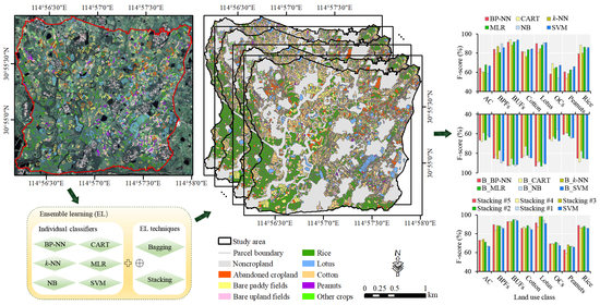
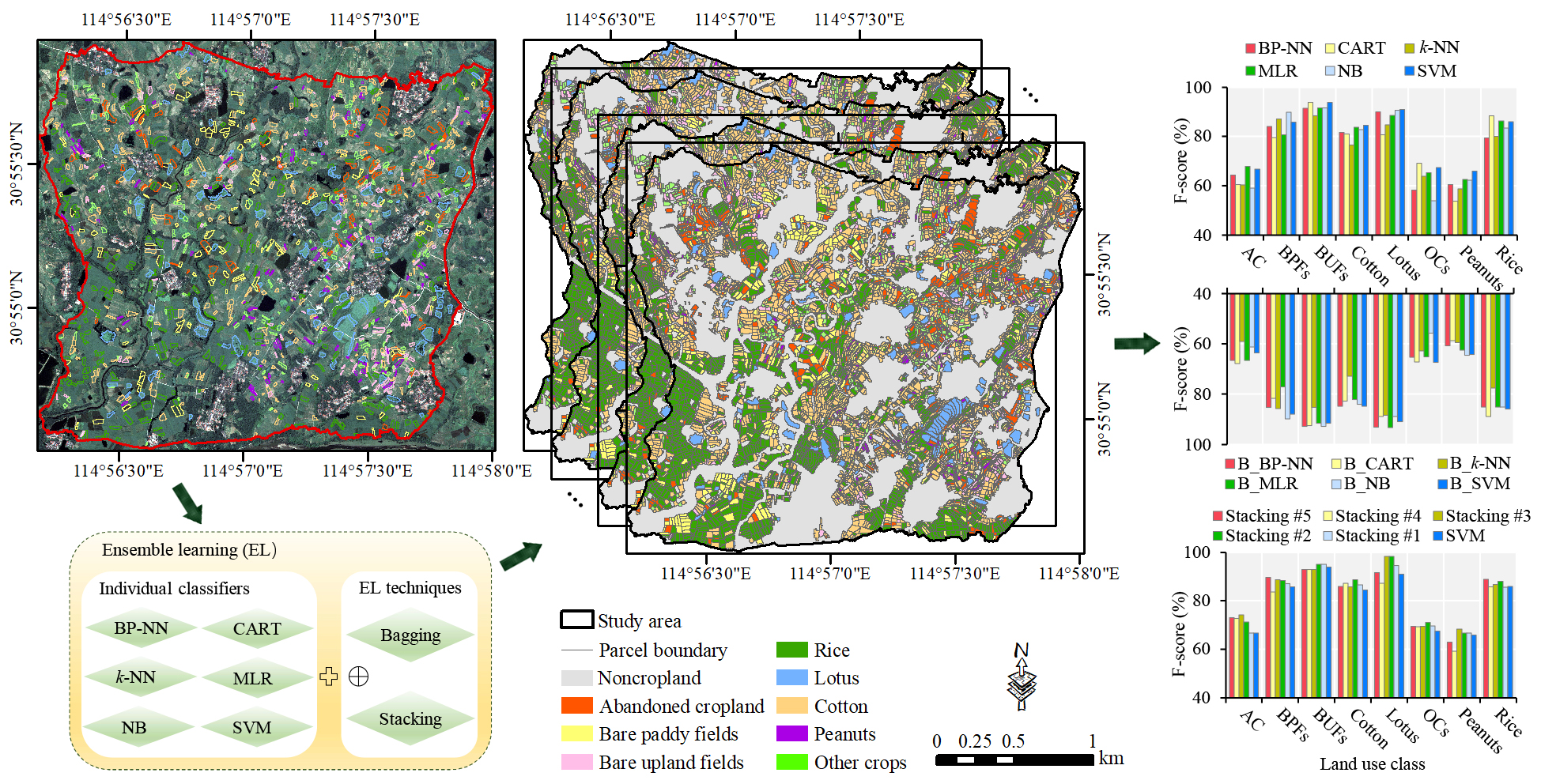
Therefore, this study aims to develop an ensemble machine learning-based framework to improve parcel-level crop mapping on smallholder farms from VHSR images. Our experiments were conducted on WV2 images from a typical smallholder agricultural area in central China. Six widely used classifiers with different basic ideas, namely, multinomial logistic regression (MLR), naive Bayes (NB) classifier, classification and regression tree (CART), backpropagation neural networks (BP-NN), k-NN, and SVM classifiers, were considered base classifiers. Bagging and stacking are typical examples of homogeneous and heterogeneous EL techniques, respectively, and therefore, were chosen to combine base classifiers. The specific objectives are to: (1) Explore how to build an appropriate ensemble model to achieve fine mapping of smallholder crops; (2) assess and compare the effects of bagging and stacking in improving the performance of individual classifiers; and (3) analyze the impact of parcel-level spatial information (e.g., textural and geometric features) extracted from VHSR images on the performance of the EL-based model.

2. Materials and Process

2.1. Study Site

The study site covers approximately 602.71 ha, 59.5% of which is occupied by farmland in the suburbs of Wuhan, Hubei Province, China (Figure 1). Located in the transition zone from the plains to the mountains and approximately 76 km northeast of downtown Wuhan, it is a typical smallholder agricultural area characterized by household-operated farms and fragmented agricultural landscapes. Cropland parcels here are generally small in size; among all of the parcels, 78.5% are smaller than 0.067 ha, while only 8.96% are larger than 0.1 ha [5]. With an elevation of 34–58 m, the terrain here slopes from the northeast to the southwest. The area has a subtropical monsoon climate, and the average monthly temperature ranges from 3.8 °C in January to 28.5 °C in July. The perennial average rainfall is 1269 mm, with extremely high annual variability. The river network system in this area is relatively developed. Abundant water resources and the warm, humid climate make it possible to grow a variety of crops throughout the year. From June to August of each year, cotton, rice, and other minor crops, such as peanuts, lotus, soybeans, sweet potatoes, and sesame, are planted here at the same time.

2.2. Data and Preprocessing

2.2.1. WorldView-2 Imagery

WV2 multispectral satellite images covering the site were collected on July 13, 2013, under clear skies (Figure 1). Every July, all of the crops reach their maximum growth, allowing for better discrimination of the crop types. In terms of the spectral resolution, WV2 can acquire images in eight spectral bands from the shorter wavelength of visible light to the near-infrared (NIR) band, namely, the four standard color bands (i.e., the blue (0.45–0.51 μm), green (0.51–0.58 μm), red (0.63–0.69 μm), and NIR1 (0.77–0.895 μm) bands) and four new bands (i.e., the coastal (0.40–0.45 μm), yellow (0.59–0.63 μm), red-edge (0.71–0.75 μm), and NIR2 (0.86–1.04 μm) bands). Figure 1 shows the true-color image of the experimental data, consisting of red, green, and blue bands. The spatial resolution of this sensor ranges from 0.5 m in the panchromatic band to 2 m in the multispectral band, with a radiometric resolution of 11 bits and a revisit period of 1.1 days.
The WV2 image was preprocessed on the ENVI 5.3 Classic® platform, including the following steps. First, radiance calibration was conducted to convert the digital number values into surface spectral reflectance values. Second, the atmospheric correction was performed using the fast line-of-sight atmospheric analysis of the spectral hypercubes module provided in ENVI 5.3 to produce top-of-canopy reflectance values. Then, the multispectral and panchromatic data were fused using the principal components spectral sharpening method. Finally, a polynomial model combining the ground control points and nearest-neighbor resampling methods was used to geometrically correct the fused 0.5-m-resolution image.

2.2.2. Parcel Boundary Vector Data

The spatial unit for this mapping task is the parcel in which the same crop is generally planted. Therefore, a vector database needs to be created that contains all of the parcel objects of the site. Parcel objects were identified and digitized on the screen using WV-2 images combined with expert knowledge and verified on site to ensure their accuracy and authenticity. Altogether, digitization resulted in 7441 cropland parcels, corresponding to 359.50 ha, accounting for approximately 59.5% of the site area, with an average parcel area of 0.048 ha and a median parcel area of 0.037 ha [5]. To process cropland pixels only, a mask of the agricultural area was created from the parcel boundary vector layer.

2.2.3. Ground-Truth Data

Field crop type data are critical for constructing sample datasets for crop classification modeling. From July to August 2015, extensive field observations were conducted throughout the study site. To match the ground observation data with the satellite imagery, only parcels with consistent land use types for the same period in 2013 and 2015 were collected. The land use information in 2013 was obtained through interviews with local farmers, showing that consistent crop types between adjacent years were common. The types of crops grown on these parcels and their field photos were recorded. In the end, a total of 1242 cropland parcels marked with land use types were obtained, which are widely distributed and scattered (Figure 1) and could reflect the ground truth of the entire study site. Table 1 shows the different land use types and the number of parcels for each type. Furthermore, these parcels were randomly divided into training and validation sets at a ratio of 7:3. The former was used for model training, while the latter was used as an independent dataset for accuracy assessment.
Eight crop-level agricultural land use types were recorded during the field visit. Figure 2a illustrates an example of a WV2 image in RGB color mode for each land use type. Visually, there are obvious differences in the texture and hue features of the images among these land use types, providing key information for the subsequent construction of feature spaces to distinguish the crop types. Figure 2b,c show field photos of two common crops (rice and cotton), which account for the majority of the crops grown at the site. The ‘other crops’ (OCs) category generally includes sesame, soybeans, and sweet potatoes, which are classified into one category, due to their exceedingly small amount of cultivation. In addition, a small amount of abandoned cropland (AC) and some bare croplands were identified during the field visit. The latter include upland fields with bare soil and paddy fields covered with little water, but almost no crops. For the completeness of the crop-level agricultural land use classification system, we included ‘AC’, ‘bare upland fields (BUFs)’ and ‘bare paddy fields (BPFs)’ in the crop mapping system. The LULC types not observed as cropland, such as rural residential land, woodland, grassland, and water bodies, are classified as noncropland and are masked out in the image.

3. Experimental Design and Methods

3.1. Crop Mapping Framework

The proposed crop mapping approach follows the GEOBIA framework, which mainly involves four steps (Figure 3). First, image preprocessing was performed to eliminate atmospheric extinction, geometric distortion, and other uncertainties (see Section 2.2). Second, the WV2 image was segmented using the parcel boundary vector data, and a series of image features were extracted; then, Pearson’s correlation coefficient (r) and SVM recursive feature elimination (SVM-RFE) were successively applied to the initial feature set to eliminate redundant variables. Third, six widely used individual classifiers were trained using the optimal features with class labels, and then the bagging and stacking methods were applied separately to the individual classifiers to enhance their prediction performance. Fourth, the crop mapping accuracy was evaluated by calculating a confusion matrix based on independent verification data.

3.2. Feature Space Construction

3.2.1. Image Segmentation

Segmentation is related to the final quality of the ultimate thematic map, and is, therefore, a key aspect of GEOBIA. The best method is to segment the scene into objects that map features of interest in the real world [44,45]. Various image segmentation algorithms have been developed, some of which can be implemented in the form of tools or software, for instance, the multiscale segmentation algorithm provided by the eCognition platform. However, image objects automatically obtained based on these algorithms often fail to match real-world objects [30]. The mapping goal of this study focused at the parcel level to carry out crop mapping. Therefore, we used the parcel boundary vector data obtained by manual digitization to segment the WV-2 image, rather than using the existing segmentation algorithm to automatically partition the image. Image segmentation was performed on the eCognition 9.0 platform, allowing vector data to be imported for segmentation. The resulting image objects were spatially and quantitatively consistent with the cropland parcels acquired by manual digitization.

3.2.2. Feature Extraction and Selection

Image spectral information is widely used as a key variable to distinguish crop types; however, using textural and geometric features of image objects in VHSR image analysis is becoming increasingly popular [46,47,48]. To investigate whether using these spatial features can help to distinguish smallholder crop types at the parcel, in addition to 13 spectral features, 7 geometric features and 8 textural features were also extracted, based on previous studies (Table 2). Feature extraction was performed on the eCognition 9.0 platform, which provides a variety of feature variables, including all of the above types. Among them, the geometric features were generated by calculating the pixel rows of the image object, and the textural features were extracted based on the omnidirectional gray-level cooccurrence matrix (GLCM). Formulas for calculating textural features are provided in Appendix A. Regarding the spectral features, in addition to the average value of the object spectrum, as well as the maximum difference and brightness, three vegetation indices were also calculated, namely, the ratio vegetation index (RVI, Equation (1)), normalized difference vegetation index (NDVI, Equation (2)) and enhanced vegetation index (EVI, Equation (3)). The RVI, NDVI, and EVI indices were calculated from the blue, red, and NIR1 spectral bands of the WV2 images using Equations (1)–(3), respectively.
RVI = N I R 1 R e d
NDVI = N I R 1 R e d N I R 1 + R e d
EVI = 2.5 × N I R 1 R e d N I R 1 + 6 × R e d 7.5 × B l u e + 1
Feature selection aims to reduce the interference of redundant variables by selecting a subset of the existing features [52,53]. In this study, a combination strategy of ‘Pearson’s r and SVM-RFE’ was adopted. The feature selection task was performed in the following two steps. (1) Collinearity variable elimination based on a Pearson’s r threshold [54]. To weaken the effect of variable collinearity on model performance, the highly correlated variables were identified and removed by calculating Pearson’s r between each pair of existing features [55]. As a result, 11 variables with Pearson’s r greater than 0.9 or less than −0.9 were identified and removed, and the remaining 17 variables were retained (Figure 4a). (2) Target-related variable optimization based on the SVM-RFE method. As a popular wrapper-based feature selection algorithm, SVM-RFE uses the weight of the decision boundary as a metric to assess relevant features. This method performed well in similar studies [37], and was, therefore, adopted by us. A detailed introduction can be found in the report by Guyon et al. [56]. We applied SVM-RFE to the training data containing the 17 variables selected above, and evaluated the accuracy of the model using 5-fold cross-validation. As shown in Figure 4b, with the increase in the number of variables, the accuracy initially improves rapidly, tends to be stable when there are five variables, and finally reaches the maximum when there are 15 variables. Therefore, these 15 variables include six spectral features (Coastal, NIR2, NDVI, Red, Max-Diff, and EVI), five textural features (G-SD, G-mean, G-ASM, G-hom, and G-cor), and four geometric features (Area, Sha. Ind., Width, and Bor. Len.), which were ultimately determined as the optimal variables. The feature selection procedure was realized in the R 3.6.1 environment [57].

3.3. Ensemble Classification

3.3.1. Bagging and Stacking Methods

EL techniques, involving constructing and combining multiple classifiers [40], have been shown to generate better prediction or classification performance and achieve better generalization [37,39,58]. In this study, bagging and stacking were selected to combine individual classifiers, which are typical examples of homogeneous and heterogeneous EL methods, respectively. The basic ideas of the two EL methods are described below.
Bagging, short for bootstrap aggregation, generates an ensemble model by combining multiple instances of the same MLA trained on a series of random subsets of the original training data [42]. Specifically, for a full training dataset N, bagging uses the bootstrap sampling strategy to extract m sets of training subsets from N; then, m subsets are used to train the same MLA and generate m well-trained classifiers; finally, the results of these classifiers are aggregated by a voting strategy to form the final output prediction. Overall, bagging reduces the variance of the base classifier error by introducing randomness into ensemble modeling. In practice, bagging also works well with limited training data [55]. In addition, Zhou [40] suggested that bagging could enhance the performance of classifiers sensitive to small disturbances in the training set and avoid overfitting.
Stacking is another typical EL method that improves classification performance by combining multiple individual classifiers of different types [43]. In stacking, the individual classifiers participating in the combination are called base classifiers and are at level 0, and the classifier used to combine them is called the meta-classifier and is at level 1. The outline of the stacking method is as follows [59]. First, level 0 classifiers are trained separately using the original training dataset; then, a new dataset is generated, with the outputs of level 0 classifiers as the features and the original true classes still as the true classes; finally, the new dataset is used to train level 1 classifier and learn the prediction combination from level 0 classifier, thereby achieving an improved classification accuracy. Base classifiers with excellent performance and various types help the stacking model to perform well [43]. Therefore, six widely used individual classifiers with different basic ideas were selected to generate stacking models. Meta-classifiers are often simple and can provide a smooth interpretation of the predictions made by the base classifiers. As such, linear or logistic regression classifiers are often used as meta-classifiers [37]; although this practice is common, it is not required [55]. In this study, six individual classifiers were tested in turn, and the best meta-classifier was determined according to their performance.

3.3.2. Machine Learning Classifiers

Six widely used individual classifiers were selected as the base classifiers of the ensemble model, namely, BP-NN, CART, k-NN, MLR, NB, and SVM classifiers. EL models tend to perform better when the individual classifiers involved in the ensemble provide sufficient diversity of generalization patterns. That is, base classifiers must generally be accurate, and they should make mistakes in different instances. The six individual classifiers mentioned above have different basic ideas and are widely used, so they are selected as base classifiers to build EL models. These classifiers have their own merits and drawbacks, due to different working principles. For instance, as a statistical classifier based on Bayes’ theorem, the NB classifier is easy to understand and implement, but it assumes that the input variables are independent [60]. The SVM classifier is a kernel-based supervised learning method that predicts unknown values by finding the regression hyperplane closest to all of the training sets. It can achieve good performance with fewer training data and is not easy to overfit, but is rather sensitive to kernel function selection and training parameter configuration [61]. Therefore, it is expected that the classification performance can be improved by integrating these individual classifiers. Our experiments were performed on the Waikato Environment for Knowledge Analysis (WEKA), an open-source machine learning and data mining platform that provides all of the aforementioned classifiers, as well as bagging and stacking methods [62].

3.4. Accuracy Assessment

All of the constructed models were run and validated separately to evaluate their performance in the accuracy of thematic maps. For each model, by constructing a confusion matrix, standard accuracy indicators, namely, the overall accuracy (OA), user’s accuracy (UA), producer’s accuracy (PA), and kappa coefficient (kappa), were calculated (Equations (4)–(7)) [63]. Additionally, the classwise F-score (F, Equation (8)) was calculated from the harmonic mean of the PA and UA [64]. Considering the multiclass classification task, the weighted-average F-score (weighted-F, Equation (9)) was also calculated and presented. Regarding the performance comparison between the models, McNemar’s test (Equation (10)) was used to detect the statistical significance of the accuracy differences between pairs of models [65].
OA = i = 1 n p i i / p
UA ( i ) = p i i / p i +
PA ( i ) = p i i / p + i
kappa = ( i = 1 n p i i ) / p ( i = 1 n p i + p + i ) / p 2 1 ( i = 1 n p i + p + i ) / p 2
F ( i ) = 2 × UA ( i ) × PA ( i ) UA ( i ) + PA ( i )
weighted F = i = 1 n p + i p F ( i )
χ 2 = ( f A B f B A ) 2 f A B + f B A
where n and p represent the total number of classes and sample instances, respectively; p i i represents the number of correctly classified instances of the i th class; p i + represents the number of instances classified into the i th class; p + i represents the number of measured instances of the i th class; and f A B represents the number of instances that are incorrectly predicted by classifier A and correctly predicted by classifier B and vice versa for f B A .

4. Implementation and Results

4.1. Model Performance Evaluation and Comparison

4.1.1. Performance of the Individual Classifiers

Table 3 and Figure 5a summarize the performance of the six individual classifiers. The parameter profiles for these classifiers in WEKA format are provided in Appendix B. The results show that the performance of all of the individual classifiers is generally good, with the OA ranging from 75.07% to 80.70%, kappa ranging from 0.707 to 0.775, and the weighted-F ranging from 0.752 to 0.808. Specifically, the SVM classifier performed the best, followed by the MLR, CART, NB, and BP-NN classifiers, while the k-NN classifier performed the worst. Combined with the results of McNemar’s test, it can be concluded that the SVM classifier is significantly superior to other classifiers except for the MLR classifier (Figure 5d). Due to its insensitivity to the dimensionality of the sample space, the SVM classifier has been reported to be the most reliable of many off-the-shelf classifiers [66]. The performance of the MLR classifier is close to that of the SVM classifier. Previous studies have shown that MLR with the built-in LogitBoost algorithm also achieves satisfactory performance, since it allows certain inputs to be pruned by early stopping, thereby avoiding overfitting [32]. Therefore, it is not surprising that the SVM and MLR classifiers are the two best individual classifiers in our experiments.

4.1.2. Performance of the Bagging Models

The bagging method using the default parameters in WEKA (Appendix B) was separately applied to the six trained individual classifiers. The classifiers after bagging are represented as B_BP-NN, B_CART, B_k-NN, B_MLR, B_NB, and B_SVM. The results show that the effect of bagging varies by the classifier (Table 4 and Figure 5b). Compared with the performance before bagging, the classification accuracy of B_BP-NN, B_CART, and B_NB was significantly improved (Figure 5d). Among them, B_BP-NN underwent the greatest improvement, and its OA increased from 76.41% to 79.89%; moreover, B_CART, and B_NB also achieved better performances, although the improvement in accuracy was small, and their OAs increased from 78.02% and 77.21% to 79.89% and 78.55%, respectively. These experimental results indicate that the bagging method is particularly useful for improving the performance of neural networks or tree-based classifiers, consistent with the findings of Kim and Kang [67]. In contrast, compared with the performance before bagging, the classification accuracy of B_k-NN, B_MLR, and B_SVM decreased slightly, but the decrease was not significant (Figure 5d). The OA and kappa values of B_SVM were still greater than those with the other bagging models (Table 4). Nevertheless, the results of McNemar’s test show that, except for B_k-NN, there was no significant difference in accuracy between B_SVM and the other bagging models (Figure 5d). In short, these experiments on the WV2 dataset show that, although bagging can moderately improve the performance of unstable classifiers, the improvement is limited, narrowing only the accuracy gap between the ‘bad’ classifiers and the ‘good’ classifiers. Therefore, we attempted to use the stacking EL method to improve the accuracy of crop mapping.

4.1.3. Performance of the Stacking Models

After several experiments, the SVM was determined to be the best meta-classifier to integrate individual classifiers. We first sorted the individual classifiers in descending order of OA (i.e., SVM > MLR > CART > NB > BP-NN > k-NN) and then combined them into five combinations: #1: SVM + MLR; #2: SVM + MLR + CART; #3: SVM + MLR + CART + NB; #4: SVM + MLR + CART + NB + BP-NN; #5: SVM + MLR + CART + NB + BP-NN + k-NN. Subsequently, six individual classifiers were tested separately as meta-classifiers to implement the stack method to relearn the predictions from #1 to #5. A total of 30 models were generated, and their accuracy evaluations are presented in Appendix C. We found that the SVM as a meta-classifier ensured the most accurate results. The five stacking models with the SVM as the meta-classifier are denoted as: Stacking #1 to #5. Appendix B provides the detailed parameter configurations for the five stacking models.
The performance of the five stacking models are shown in Table 5 and Figure 5c. The results show that the classification accuracy of Stacking #1 (OA = 82.04%, and kappa = 0.790) was already greater than that of the SVM and MLR classifiers (Table 3). After the CART classifier was added (Stacking #2), the OA and kappa values increased to 83.91% and 0.812, respectively. However, the accuracy could not be further improved and declined somewhat after the NB and BP-NN classifiers were successively added to the stacking models (i.e., Stackings #3 and #4). Stacking #5 is an ensemble of all of the individual classifiers, and its performance was better than those of Stacking #1 and Stacking #4, but slightly worse than those of Stacking #2 and Stacking #3.

4.1.4. Comparison of the Stacking with Other Models

The accuracy evaluation results showed that the stacking models using the SVM as the meta-classifier were superior to all of the individual classifiers and bagging models. Specifically, the OA and kappa values of all of the five stacking models were higher than those of all of the bagging models (Table 4 and Table 5). The Stacking #2 and B_SVM models performed the best in the stacking and bagging models, respectively, while the OA and kappa values of the former were 3.75% and 0.043 greater than those of the latter, respectively. Furthermore, in terms of McNemar’s test results, the Stacking #2 model was significantly better than all of the bagging models, including the B_SVM (Figure 5d).
Compared with the performance of the SVM, MLR, and CART classifiers, the OA and kappa values of the Stacking #2 model increased by 3.21% to 5.89% and 0.037 to 0.069, respectively (Table 3 and Table 5). Table 6 shows the specific accuracy index comparison between the Stacking #2 model and the three individual classifiers. The Stacking #2 model improved the F-score of all of the land use types except rice. Specifically, for AC, BPFs, BUFs, cotton, and lotus, both their PAs and UAs were improved by the Stacking #2 model; moreover, the PA of peanuts and the UA of OCs were also improved.
Overall, the Stacking #2 model showed a statistically significant advantage in accuracy over all of the other models (Figure 5d). Therefore, the Stacking #2 model could be used to generate the final crop type distribution map.

4.1.5. Comparison under Different Feature Sets

To analyze the effect of geometric and textural features on the EL-based parcel-level crop classification, we ran the Stacking #2 model on the four subsets of the optimal feature set and compared their classification performance (Table 7). Compared with using the full optimal feature set, the OA was reduced from 83.91% to 76.68%, and the kappa value was reduced from 0.812 to 0.727 when using only the spectral features. Judging from the classwise accuracy, textural and geometric features improved the accuracy of almost all of the land use types. In particular, the improvement was most pronounced in the peanut category, for which the F-score increased from 28.57% to 66.67%. In addition, compared with using only the spectral features, the crop classification accuracy was improved more significantly by adding geometric features than by adding textural features. Specifically, the addition of textural features improved only the F-scores of the AC, BPF, peanut, and rice parcels, while the addition of geometric features improved the F-scores of all of the land use types.

4.2. Predicted Crop Type Maps

4.2.1. Spatial Pattern of the Crop Types

In all of the crop maps predicted by the Stacking #2 model and the three classifiers involved in the model, cotton and rice crops dominated the study site (Figure 6a–d). According to the statistics of the optimal predicted map (Figure 6a), the proportions of rice, cotton, lotus, peanuts, and OCs in the entire cropland area are 27.70%, 37.67%, 5.38%, 2.59%, and 5.25%, respectively. In addition, the BUF, BPF, and AC amounts cannot be ignored, accounting for 8.27%, 4.45%, and 8.69%, respectively. Judging from the spatial distribution, rice is concentrated in the southwestern part of the site, where water sources are abundant and easy to irrigate, while cotton is mainly concentrated in the northern and eastern parts, which have a higher terrain. Peanuts and OCs are commonly interlaced with cotton. There are relatively few lotus parcels, which are scattered in the middle of the site. We also found that AC parcels are mainly located in the northeastern part of the site, where the parcels are easy to abandon, likely because of the high terrain and inconvenient irrigation. In short, various crops are scattered over broken farmland, which is a typical portrayal of smallholder farms in central China.

4.2.2. Agreement Analysis of the Prediction Maps

The positions of agreement and disagreement in terms of the predictions of the four classifiers are shown in Figure 7a. Of the 7441 parcels, the class allocations agreed upon by the four classifiers accounted for the majority, approximately 74.77% (Figure 7b). For approximately 18.09% of the parcels, three of the four classifiers agreed on their predictions. There were two cases in which only two classifiers agreed on the class allocations, expressed as AABB (4.19%) and AABC (2.65%). The former means that two of the four classifiers agree with A, and the other two agree with B; the latter means that two classifiers agree with A, and the other two classifiers disagree with A and with each other. In addition, there is an extremely small proportion of parcels for which the predictions of the four classifiers disagree with each other. These disagreements mostly occurred in the complex planting areas in the eastern part of the site. The agreement map of the selected area and the corresponding WV2 image are presented in Figure 7c, and the corresponding partial crop maps are shown in Figure 7d.

4.2.3. Error Analysis of the Prediction Maps

The confusion between peanuts and OCs was the main source of error in the crop prediction maps. Figure 8 is a visual display of errors generated by Stacking #2 and the other three individual classifiers. Of all of the predictions made by the four classifiers, the most serious confusion occurred between peanuts and OCs. The consequence of this confusion was the low F-scores of peanuts (53.73–66.67%) and OCs (65.22–70.97%) (Table 6). In addition, in the predicted crop map, AC was easily confused with land use types other than BUFs and peanut fields. Fortunately, this confusion was effectively reduced by implementing the stacking method, and the F-score of AC increased from 60.38% to 71.19% (Table 6). The crop confusion mentioned above was partly caused by the complex cropping practices of smallholder farms. Especially for peanuts, sesame, sweet potatoes, and other minor crops, their growth cycles in the study site were remarkably similar, and intercropping patterns generally existed among these crops. Therefore, it was difficult to distinguish peanuts from OCs. Regarding AC, although these parcels have been consciously abandoned by farmers, some parcels still have sparse crops growing naturally, due to residual seeds, which might explain why it is confused with other land use types.

5. Discussions

5.1. Advantages of the Stacking Ensemble

By combining multiple individual classifiers of different types using the stacking method, the mapping accuracy of parcel-level smallholder crops was improved. Specifically, compared with the performance of the individual classifiers, the OA of the Stacking #2 model, which uses the SVM as a meta-classifier to integrate the three best-performing individual classifiers, increased by 3.21% to 5.89% (Table 6), and the classwise accuracy was also improved for almost all of the land use types. These improvements are due to the stacking model relearning the predictions of the individual classifiers [43]. One can note that the performance of these three individual classifiers varies with the land use type (Table 6). Specifically, the SVM classifier performed well on the BPF, BUF, cotton, lotus, and peanut parcels; MLR performed well on AC; and CART performed well on the BUF, OC, and rice parcels. In general, it is precisely because of the high-level and differentiated performance of the individual classifiers involved in the integration that the stacking model has outstanding performance.
In the existing studies, there is generally no clear method to determine the appropriate meta-classifier. In practice, majority voting strategies [39], linear regression [37], and stochastic gradient boosting [55] algorithms have all been used as meta-classifiers to combine individual classifiers. In this study, six commonly used individual classifiers were tested, and the SVM was found to perform best as a meta-classifier. In short, there is no universal optimal meta-classifier, and it often depends on the data structure used and should be determined by extensive comparative experiments. Individual classifiers with the best predictive performance, such as the SVM in this study, or classifiers with the simplest basic ideas, such as linear or logistic regression, can be preferred as meta-classifiers for stacking models.
Determining the appropriate base classifiers is another key to causing the stacking method to perform well. Previous studies have shown that sufficiency and diversity are two important criteria for selecting the appropriate base classifiers [59], indicating that each base classifier should have good predictive ability, and the dependence between them should be minimized to provide complementary information [37]. In this study, six individual classifiers were added to the stacking learner one by one in descending order of classification accuracy. With the successive addition of base classifiers, the performance of the stacking model changed from improvement to deterioration (see Table 5). In the end, the SVM, MLR, and CART were identified as the best base classifiers because the Stacking #2 model integrating them had the optimal performance. Moreover, we also found that the stacking model that uses the SVM as a meta-classifier and combines all of the individual classifiers has no obvious advantage in classification accuracy. Of all of the five stacking models, the best-performing model integrates the best three individual classifiers (Stacking #2), not the model that combines all six classifiers (Stacking #5). Therefore, when building a stacking model, one should be cautious when introducing base classifiers and should not include all of the available classifiers. In this context, combining the available individual classifiers in descending order of accuracy and comparing the performance of the constructed stacking models could be an effective way to determine the best base classifiers.

5.2. Effect of the Bagging Ensemble

The behavior of the bagging method varies depending on the individual classifier. Many studies have shown that off-the-shelf bagging classifiers, such as the most representative RF classifier, perform well in image classification examples [12,58]. In this study, six self-assembled bagging models were generated by applying the bagging method to the six trained individual classifiers. Through comparative analysis, it was found that the bagging method slightly improved the performance of the BP-NN, CART, and NB classifiers. This finding further supports the view that the bagging method can work better on weak classifiers that are sensitive to disturbances [41,55]. The reason is that by introducing randomness in the sampling process, bagging can reduce the error variance of the unstable base classifier [42]. Although the k-NN classifier performed poorly in this study, the bagging method failed to improve its classification accuracy. This phenomenon might be due to the insensitivity of the k-NN classifier to disturbances in the training samples [66]. In addition, it was also found that applying the bagging method to the better-performing SVM and MLR classifiers failed to improve their performance, but rather reduced it. The reason could be that the B_SVM and B_MLR models overfit the training dataset, especially for good instances [41].
Whether the tree-based bagging classifier performs better than the kernel-based classifier remains debatable [55]. The most typical debate is the dispute between the RF and SVM classifiers [68]. Interestingly, our experiments show that the performance of the tree-based bagging classifier (i.e., B_CART) is still inferior to that of an SVM with a radial basis function kernel. However, there are many types of tree-based bagging classifiers, and a variety of kernel functions are available for the SVM, so similar comparative experiments must be performed more extensively in the future.

5.3. Contribution of the Spatial Features

Although many studies have shown that the geometric and textural information provided by VHSR images is very useful for improving the accuracy of crop mapping [12,46]; some studies have reported that the effectiveness of these features is not obvious [69]. Our experiments demonstrate that the performance of the classifier can be significantly enhanced using these spatial features in mapping complex agricultural landscapes from VHSR images. This benefits from using these features can increase the discrimination dimension of the crop types, thereby better-addressing data variability in complex heterogeneous landscapes [12]. For the hard-to-identify peanut, OC, and AC parcels in this study, their F-scores increased by 38.10%, 7.18%, and 12.73% (Table 7), respectively, after the geometric and textural features of the image objects were used. Such information could be helpful for image feature selection in similar parcel-level crop mapping tasks.

5.4. Benefits/Drawbacks of Our Approach

By making full use of the VHSR images and integrating individual classifiers, the accuracy of parcel-level smallholder crop mapping has been moderately improved. Specifically, several ensemble models were built by implementing bagging and stacking methods on six individual classifiers, and they were applied to the mapping of parcel-level smallholder crops in central China. Among all the models, the Stacking #2 model, which integrated the SVM, MLR, and CART classifiers, performed the best. Compared with the performance of the individual classifiers, the Stacking #2 model improved the classwise accuracy of almost all of the land use types. Since the classification performance can be significantly improved without adding costly data collection, the stacking ensemble method is valuable for accurately mapping smallholder crops. In addition, compared with previous similar studies at the same study site [5], we achieved greater mapping accuracy with fewer feature variables through further feature optimization and ensemble classification. The ensemble machine-learning-based framework proposed in this study could provide an effective approach for fine-scale crop mapping in similar complex agricultural areas, which is beneficial to the development of the local RS-based crop identification system.
Although the ensemble models achieve high performance, there is still the potential for further improving the mapping accuracy of smallholder crops. In this study, the confusion between peanuts and OCs caused their classification accuracies to be relatively low. Using EL techniques on individual classifiers, we have moderately improved their classwise accuracies, but this improvement has not changed their accuracy rankings. In other words, crops that were easily confused by the individual classifiers were still easily confused by the ensemble models. While this confusion has been moderately reduced, it has not yet been completely eliminated. Therefore, the accurate distinction between confusingly minor crops, such as peanuts and OCs, requires further research. This confusion is often caused by the complex planting practices in smallholder agricultural areas [70]. Specifically, OCs, including sweet potatoes, soybeans, sesame, and other minor crops, had the same growing period as peanuts at this site, and there was generally a certain proportion of intercropping patterns among them. Therefore, seeking or developing appropriate methods to map this intercropping pattern, thereby future research should focus on improving the mapping accuracy of smallholder crops.
The dependence on parcel boundary data limits the application of the proposed methodological framework in large regions. Automatic extraction of parcel boundary information has always been a challenge in the field of agricultural RS [45,71]. Although there are many automatic and semiautomatic object-oriented image segmentation methods [30], it remains difficult to use these methods to segment images to extract homogeneous and complete parcels [44]. Therefore, in this study, we chose to obtain parcel boundary data through manual digitization. However, this method will generate very large and expensive workloads in large-area applications. Therefore, for areas where ready-made parcel boundary data are not available, the proposed approach might be suitable only for small-area applications, such as sampling areas.

6. Conclusions

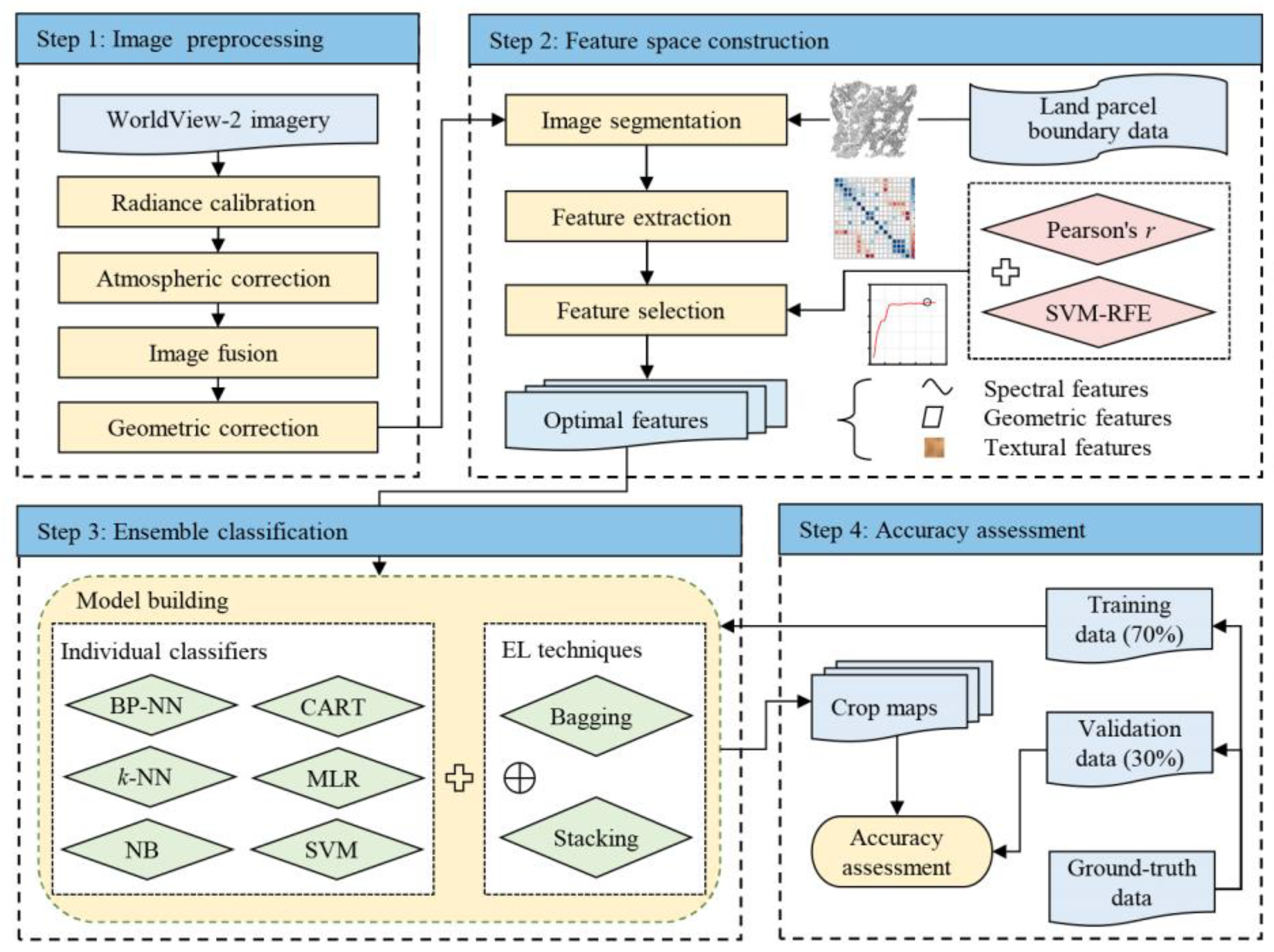
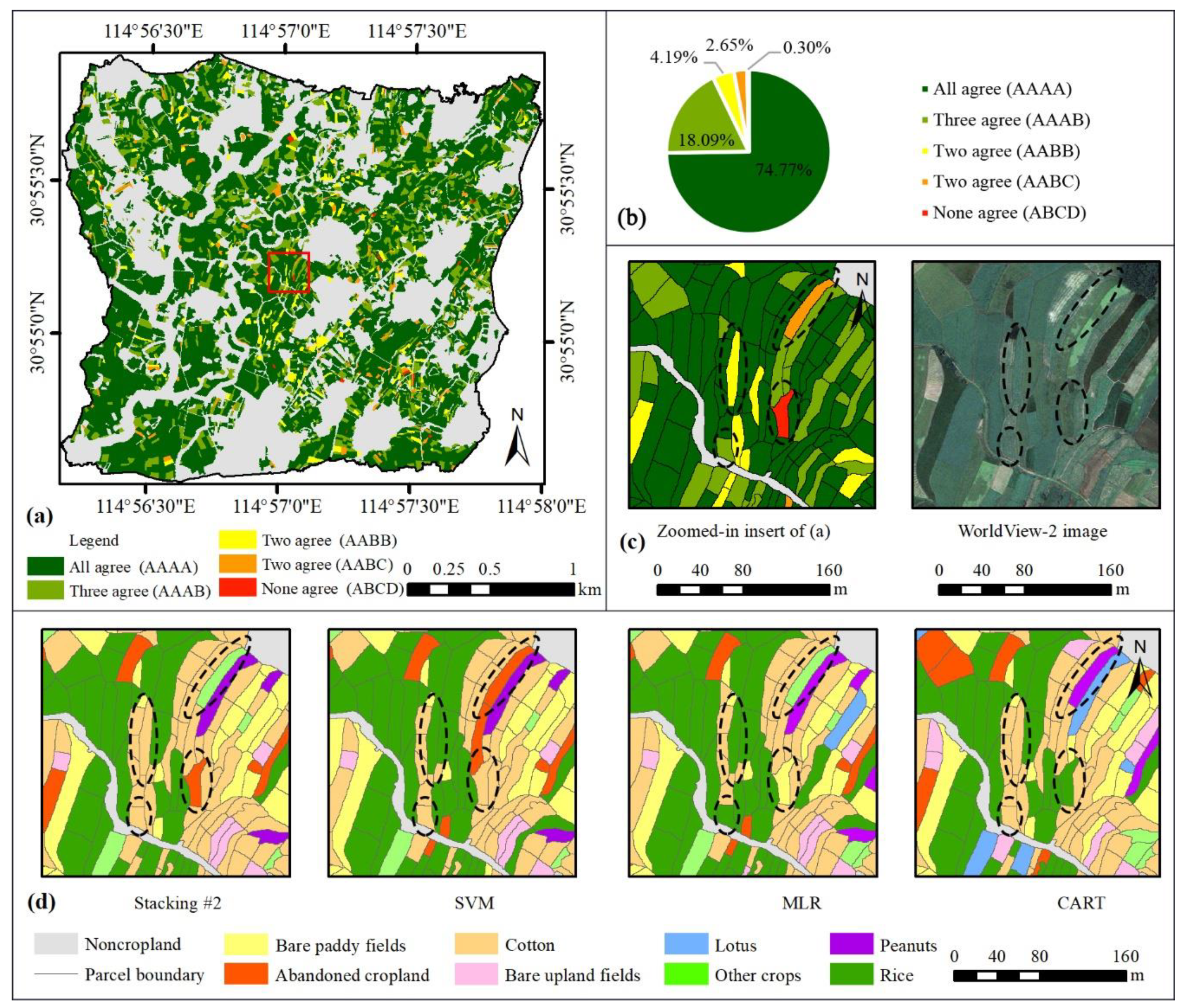
Timely and accurate mapping of smallholder crops at the parcel level is essential for predicting grain yields and formulating area-based subsidies. In this study, an ensemble machine-learning-based framework was presented to improve the accuracy of parcel-level smallholder crop mapping from VHSR images. Several ensemble models were built by applying bagging and stacking approaches separately on six widely used individual classifiers. The comparative experiments showed that the stacking approach was superior to the bagging approach in improving the mapping accuracy of smallholder crops based on individual classifiers. The bagging models enhanced the performance of classifiers with tree structures or neural networks (e.g., CART and BP-NN), but these improvements were limited in that they narrowed only the accuracy gap between the ‘bad’ classifiers and the ‘good’ classifiers. The stacking models tended to perform better, and the Stacking #2 model, which uses the SVM as a meta-classifier to integrate the three best-performing individual classifiers (i.e., SVM, MLR, and CART), performed the best among all of the built models and improved the classwise accuracy of almost all of the land use types. This ensemble approach does not require additional costly sampling and specialized equipment, and improvements in mapping accuracy are clearly valuable for the delicacy management of smallholder crops. In addition, we also proved that using the spatial features of image objects can improve the accuracy of parcel-level smallholder crop mapping. In summary, the proposed framework shows the great potential of combining ensemble learning technology with VHSR images for accurate mapping of smallholder crops, which could facilitate the development of parcel-level crop identification systems in countries dominated by smallholder agriculture.
Although these experiments focused on smallholder farms in central China, the methodological framework presented in this study could easily be applied to other similarly complex and heterogeneous agricultural areas. In the future, methods for mapping intercropping and mixed-cropping patterns need to be developed to improve the classification accuracy of smallholder crops. In addition, independent of the classifier integration, image composition accounting for phenology to support dynamic mapping of smallholder crops needs further research.

Author Contributions

Conceptualization, S.H. and P.Z.; methodology, P.Z. and W.L.; software, P.Z. and P.C.; writing—original draft preparation, P.Z.; writing—review and editing, S.H., W.L. and C.Z.; visualization, P.Z. and P.C.; supervision, S.H. and C.Z.; funding acquisition, S.H. All authors have read and agreed to the published version of the manuscript.

Funding

This research was funded by the Major Project from the National Social Science Foundation of China (Grant No. 18ZDA053).

Informed Consent Statement

Not applicable.

Data Availability Statement

The data presented in this study are available on request from the corresponding author.

Acknowledgments

We are grateful to the other members of the research team led by Shougeng Hu for their support in field data collection. We also thank the four reviewers for their insightful suggestions and comments.

Conflicts of Interest

The authors declare no conflict of interest.

Appendix A. Texture Metrics

Table A1. Formulas for calculating textural features from gray-level cooccurrence matrix.
No.Texture MeasuresFormula
1Homogeneity i , j = 0 N 1 ( P i , j / ( 1 + ( i j ) 2 ) )
2Contrast i , j = 0 N 1 P i , j ( i j ) 2
3Dissimilarity i , j = 0 N 1 P i , j i j
4Entropy i , j = 0 N 1 P i , j ( ln P i , j )
5Ang. 2nd moment i , j = 0 N 1 P i , j 2
6Mean μ i = i , j = 0 N 1 i ( P i , j ) ; μ j = i , j = 0 N 1 j ( P i , j )
7Standard deviation σ i = i , j = 0 N 1 P i , j ( i μ i ) 2 ; σ j = i , j = 0 N 1 P i , j ( j μ j ) 2
8Correlation i , j = 0 N 1 P i , j ( i μ i ) ( j μ j ) / σ i σ j
Note: P i , j = V i , j / i , j = 0 N 1 V i , j , where V i , j is the value in the cell i , j (row i and column j ) of the moving window and N is the number of columns or rows.

Appendix B. Model’s Parameter Configuration

Below is the download link of the WEKA parameter configuration files for the individual classifiers, namely, BP-NN, CART, k-NN, MLR, NB, and SVM:
Below is the download link of the WEKA parameter configuration files for the bagging models, namely, B_BP-NN, B_CART, B_k-NN, B_MLR, B_NB, and B_SVM:
Below is the download link of the WEKA parameter configuration files for the Stacking #1 to #5 models:

Appendix C. Comparison under Different Meta-Classifiers

Table A2. Overall accuracies and kappa values of the stacking methods using different meta-classifiers and base classifiers.
Meta-ClassifiersBase Classifiers
#1#2#3#4#5
OA (%)KappaOA (%)KappaOA (%)KappaOA (%)KappaOA (%)Kappa
SVM *82.040.79083.910.81283.110.80380.970.77882.570.796
MLR80.970.77782.040.7979.620.76277.210.73575.070.710
CART74.260.69974.260.69976.140.72275.340.71278.280.747
NB68.360.63578.280.74768.100.63367.290.62467.830.630
BP-NN80.430.77281.500.78380.700.77480.430.77180.160.768
k-NN80.700.74481.230.7880.160.76881.500.78480.700.775
Note: #1: SVM + MLR. #2: SVM + MLR + CART. #3: SVM + MLR + CART + NB. #4: SVM + MLR + CART + NB + BP-NN. #5: SVM + MLR + CART + NB + BP-NN + k-NN. * The SVM was finally determined as the best meta-classifier.

References

  1. ETC Group. Who Will Feed Us? Questions for the Food and Climate Crisis; ETC Group Communiqué: Ottawa, ON, Canada, 2009. [Google Scholar]
  2. Wolfenson, K.D.M. Coping with the Food and Agriculture Challenge: Smallholders’ Agenda; FAO: Rome, Italy, 2013. [Google Scholar]
  3. Bermeo, A.; Couturier, S.; Pizaña, M.G. Conservation of traditional smallholder cultivation systems in indigenous territories: Mapping land availability for milpa cultivation in the Huasteca Poblana, Mexico. Appl. Geogr. 2014, 53, 299–310. [Google Scholar] [CrossRef]
  4. Lambert, M.J.; Traoré, P.C.S.; Blaes, X.; Baret, P.; Defourny, P. Estimating smallholder crops production at village level from Sentinel-2 time series in Mali’s cotton belt. Remote Sens. Environ. 2018, 216, 647–657. [Google Scholar] [CrossRef]
  5. Zhang, P.; Hu, S.; Li, W.; Zhang, C. Parcel-level mapping of crops in a smallholder agricultural area: A case of central China using single-temporal VHSR imagery. Comput. Electron. Agric. 2020, 175, 105581. [Google Scholar] [CrossRef]
  6. Kamal, M.; Schulthess, U.; Krupnik, T.J. Identification of mung bean in a smallholder farming setting of coastal south asia using manned aircraft photography and sentinel-2 images. Remote Sens. 2020, 12, 3688. [Google Scholar] [CrossRef]
  7. Morton, J.F. The impact of climate change on smallholder and subsistence agriculture. Proc. Natl. Acad. Sci. USA 2007, 104, 19680–19685. [Google Scholar] [CrossRef] [Green Version]
  8. Lei, Y.; Liu, C.; Zhang, L.; Luo, S. How smallholder farmers adapt to agricultural drought in a changing climate: A case study in southern China. Land Use Pol. 2016, 55, 300–308. [Google Scholar] [CrossRef]
  9. Chandra, A.; Mcnamara, K.E.; Dargusch, P.; Maria, A.; Dalabajan, D. Gendered vulnerabilities of smallholder farmers to climate change in conflict-prone areas: A case study from Mindanao, Philippines. J. Rural Stud. 2017, 50, 45–59. [Google Scholar] [CrossRef]
  10. Jin, Z.; Azzari, G.; You, C.; Di, S.; Aston, S.; Burke, M.; Lobell, D.B. Smallholder maize area and yield mapping at national scales with Google Earth Engine. Remote Sens. Environ. 2019, 228, 115–128. [Google Scholar] [CrossRef]
  11. Piiroinen, R.; Heiskanen, J.; Mõttus, M.; Pellikka, P. Classification of crops across heterogeneous agricultural landscape in Kenya using AisaEAGLE imaging spectroscopy data. Int. J. Appl. Earth Obs. Geoinf. 2015, 39, 1–8. [Google Scholar] [CrossRef]
  12. Lebourgeois, V.; Dupuy, S.; Vintrou, É.; Ameline, M.; Butler, S.; Bégué, A. A combined random forest and OBIA classification scheme for mapping smallholder agriculture at different nomenclature levels using multisource data (simulated Sentinel-2 time series, VHRS and DEM). Remote Sens. 2017, 9, 259. [Google Scholar] [CrossRef] [Green Version]
  13. Breunig, F.M.; Galvão, L.S.; Dalagnol, R.; Santi, A.L.; Della-Flora, D.P.; Chen, S. Assessing the effect of spatial resolution on the delineation of management zones for smallholder farming in southern Brazil. Remote Sens. Appl. Soc. Environ. 2020, 100325. [Google Scholar]
  14. Conrad, C.; Löw, F.; Lamers, J.P.A. Mapping and assessing crop diversity in the irrigated Fergana Valley, Uzbekistan. Appl. Geogr. 2017, 86, 102–117. [Google Scholar] [CrossRef]
  15. Liu, X.; Zhai, H.; Shen, Y.; Lou, B.; Jiang, C.; Li, T.; Hussain, S.B.; Shen, G. Large-Scale Crop Mapping from Multisource Remote Sensing Images in Google Earth Engine. IEEE J. Sel. Top. Appl. Earth Obs. Remote Sens. 2020, 13, 414–427. [Google Scholar] [CrossRef]
  16. Leroux, L.; Jolivot, A.; Bégué, A.; Lo Seen, D.; Zoungrana, B. How reliable is the MODIS land cover product for crop mapping Sub-Saharan agricultural landscapes? Remote Sens. 2014, 6, 8541–8564. [Google Scholar] [CrossRef] [Green Version]
  17. Liu, L.; Xiao, X.; Qin, Y.; Wang, J.; Xu, X.; Hu, Y.; Qiao, Z. Mapping cropping intensity in China using time series Landsat and Sentinel-2 images and Google Earth Engine. Remote Sens. Environ. 2020, 239, 111624. [Google Scholar] [CrossRef]
  18. Planque, C.; Lucas, R.; Punalekar, S.; Chognard, S.; Hurford, C.; Owers, C.; Horton, C.; Guest, P.; King, S.; Williams, S.; et al. National Crop Mapping Using Sentinel-1 Time Series: A Knowledge-Based Descriptive Algorithm. Remote Sens. 2021, 13, 846. [Google Scholar] [CrossRef]
  19. Alganci, U.; Sertel, E.; Ozdogan, M.; Ormeci, C. Parcel-level identification of crop types using different classification algorithms and multi-resolution imagery in Southeastern Turkey. Photogramm. Eng. Remote Sensing. 2013, 79, 1053–1065. [Google Scholar] [CrossRef]
  20. Kussul, N.; Lemoine, G.; Gallego, F.J.; Skakun, S.V.; Lavreniuk, M.; Shelestov, A.Y. Parcel-Based Crop Classification in Ukraine Using Landsat-8 Data and Sentinel-1A Data. IEEE J. Sel. Top. Appl. Earth Obs. Remote Sens. 2016, 9, 2500–2508. [Google Scholar] [CrossRef]
  21. Sitokonstantinou, V.; Papoutsis, I.; Kontoes, C.; Arnal, A.L.; Andrés, A.P.A.; Zurbano, J.A.G. Scalable parcel-based crop identification scheme using Sentinel-2 data time-series for the monitoring of the common agricultural policy. Remote Sens. 2018, 10, 911. [Google Scholar] [CrossRef] [Green Version]
  22. Das, K.; Pramanik, D.; Santra, S.C.; Sengupta, S. Parcel wise crop discrimination and web based information generation using remote sensing and open source software. Egypt. J. Remote Sens. Sp. Sci. 2019, 22, 117–125. [Google Scholar] [CrossRef]
  23. Neigh, C.S.R.; Carroll, M.L.; Wooten, M.R.; McCarty, J.L.; Powell, B.F.; Husak, G.J.; Enenkel, M.; Hain, C.R. Smallholder crop area mapped with wall-to-wall WorldView sub-meter panchromatic image texture: A test case for Tigray, Ethiopia. Remote Sens. Environ. 2018, 212, 8–20. [Google Scholar] [CrossRef]
  24. Zhang, D.; Pan, Y.; Zhang, J.; Hu, T.; Zhao, J.; Li, N.; Chen, Q. A generalized approach based on convolutional neural networks for large area cropland mapping at very high resolution. Remote Sens. Environ. 2020, 247, 111912. [Google Scholar] [CrossRef]
  25. Hay, G.J.; Castilla, G. Geographic Object-Based Image Analysis (GEOBIA): A new name for a new discipline. In Object-Based Image Analysis; Springer: Berlin/Heidelberg, Germany, 2008; pp. 75–89. [Google Scholar]
  26. Arvor, D.; Durieux, L.; Andrés, S.; Laporte, M.A. Advances in Geographic Object-Based Image Analysis with ontologies: A review of main contributions and limitations from a remote sensing perspective. ISPRS J. Photogramm. Remote Sens. 2013, 82, 125–137. [Google Scholar] [CrossRef]
  27. Vaudour, E.; Noirot-Cosson, P.E.; Membrive, O. Early-season mapping of crops and cultural operations using very high spatial resolution Pléiades images. Int. J. Appl. Earth Obs. Geoinf. 2015, 42, 128–141. [Google Scholar] [CrossRef]
  28. Wu, M.; Huang, W.; Niu, Z.; Wang, Y.; Wang, C.; Li, W.; Hao, P.; Yu, B. Fine crop mapping by combining high spectral and high spatial resolution remote sensing data in complex heterogeneous areas. Comput. Electron. Agric. 2017, 139, 1–9. [Google Scholar] [CrossRef]
  29. Tang, Z.; Wang, H.; Li, X.; Li, X.; Cai, W.; Han, C. An object-based approach for mapping crop coverage using multiscale weighted and machine learning methods. IEEE J. Sel. Top. Appl. Earth Obs. Remote Sens. 2020, 13, 1700–1713. [Google Scholar] [CrossRef]
  30. Hossain, M.D.; Chen, D. Segmentation for Object-Based Image Analysis (OBIA): A review of algorithms and challenges from remote sensing perspective. ISPRS J. Photogramm. Remote Sens. 2019, 150, 115–134. [Google Scholar] [CrossRef]
  31. Maxwell, A.E.; Warner, T.A.; Fang, F. Implementation of machine-learning classification in remote sensing: An applied review. Int. J. Remote Sens. 2018, 39, 2784–2817. [Google Scholar] [CrossRef] [Green Version]
  32. Peña, J.M.; Gutiérrez, P.A.; Hervás-Martínez, C.; Six, J.; Plant, R.E.; López-Granados, F. Object-based image classification of summer crops with machine learning methods. Remote Sens. 2014, 6, 5019–5041. [Google Scholar] [CrossRef] [Green Version]
  33. Feng, S.; Zhao, J.; Liu, T.; Zhang, H.; Zhang, Z.; Guo, X. Crop Type Identification and Mapping Using Machine Learning Algorithms and Sentinel-2 Time Series Data. IEEE J. Sel. Top. Appl. Earth Obs. Remote Sens. 2019, 12, 3295–3306. [Google Scholar] [CrossRef]
  34. Xu, L.; Zhang, H.; Wang, C.; Zhang, B.; Liu, M. Crop classification based on temporal information using Sentinel-1 SAR time-series data. Remote Sens. 2019, 11, 53. [Google Scholar] [CrossRef] [Green Version]
  35. Feyisa, G.L.; Palao, L.K.; Nelson, A.; Gumma, M.K.; Paliwal, A.; Win, K.T.; Nge, K.H.; Johnson, D.E. Characterizing and mapping cropping patterns in a complex agro-ecosystem: An iterative participatory mapping procedure using machine learning algorithms and MODIS vegetation indices. Comput. Electron. Agric. 2020, 175, 105595. [Google Scholar] [CrossRef]
  36. Pal, M. Ensemble learning with decision tree for remote sensing classification. World Acad. Sci. Eng. Technol. 2007, 36, 258–260. [Google Scholar]
  37. Feng, L.; Zhang, Z.; Ma, Y.; Du, Q.; Williams, P.; Drewry, J.; Luck, B. Alfalfa yield prediction using UAV-based hyperspectral imagery and ensemble learning. Remote Sens. 2020, 12, 2028. [Google Scholar] [CrossRef]
  38. Khosravi, I.; Safari, A.; Homayouni, S.; McNairn, H. Enhanced decision tree ensembles for land-cover mapping from fully polarimetric sar data. Int. J. Remote Sens. 2017, 38, 7138–7160. [Google Scholar] [CrossRef]
  39. Man, C.D.; Nguyen, T.T.; Bui, H.Q.; Lasko, K.; Nguyen, T.N.T. Improvement of land-cover classification over frequently cloud-covered areas using landsat 8 time-series composites and an ensemble of supervised classifiers. Int. J. Remote Sens. 2018, 39, 1243–1255. [Google Scholar] [CrossRef]
  40. Zhou, Z.-H. Ensemble Methods: Foundations and Algorithms; CRC Press: Boca Raton, FL, USA, 2012; ISBN 1439830037. [Google Scholar]
  41. Wang, G.; Hao, J.; Ma, J.; Jiang, H. A comparative assessment of ensemble learning for credit scoring. Expert Syst. Appl. 2011, 38, 223–230. [Google Scholar] [CrossRef]
  42. Breiman, L. Bagging predictors. Mach. Learn. 1996, 24, 123–140. [Google Scholar] [CrossRef] [Green Version]
  43. Wolpert, D.H. Stacked generalization. Neural Netw. 1992, 5, 241–259. [Google Scholar] [CrossRef]
  44. Watkins, B.; Van Niekerk, A. A comparison of object-based image analysis approaches for field boundary delineation using multi-temporal Sentinel-2 imagery. Comput. Electron. Agric. 2019, 158, 294–302. [Google Scholar] [CrossRef]
  45. Hong, R.; Park, J.; Jang, S.; Shin, H.; Kim, H.; Song, I. Development of a Parcel-Level Land Boundary Extraction Algorithm for Aerial Imagery of Regularly Arranged Agricultural Areas. Remote Sens. 2021, 13, 1167. [Google Scholar] [CrossRef]
  46. Peña-Barragán, J.M.; Ngugi, M.K.; Plant, R.E.; Six, J. Object-based crop identification using multiple vegetation indices, textural features and crop phenology. Remote Sens. Environ. 2011, 115, 1301–1316. [Google Scholar] [CrossRef]
  47. Ursani, A.A.; Kpalma, K.; Lelong, C.C.D.; Ronsin, J. Fusion of textural and spectral information for tree crop and other agricultural cover mapping with very-high resolution satellite images. IEEE J. Sel. Top. Appl. Earth Obs. Remote Sens. 2012, 5, 225–235. [Google Scholar] [CrossRef]
  48. Ma, L.; Cheng, L.; Li, M.; Liu, Y.; Ma, X. Training set size, scale, and features in Geographic Object-Based Image Analysis of very high resolution unmanned aerial vehicle imagery. ISPRS J. Photogramm. Remote Sens. 2015, 102, 14–27. [Google Scholar] [CrossRef]
  49. Jordan, C.F. Derivation of Leaf-Area Index from Quality of Light on the Forest Floor. Ecology. 1969, 50, 663–666. [Google Scholar] [CrossRef]
  50. Rouse, J.W., Jr.; Haas, R.H.; Schell, J.A.; Deering, D.W. Monitoring vegetation systems in the great plains with erts; NASA Special Publication: Washington, DC, USA, 1974. [Google Scholar]
  51. Huete, A.; Didan, K.; Miura, T.; Rodriguez, E.P.; Gao, X.; Ferreira, L.G. Overview of the radiometric and biophysical performance of the MODIS vegetation indices. Remote Sens. Environ. 2002, 83, 195–213. [Google Scholar] [CrossRef]
  52. Löw, F.; Michel, U.; Dech, S.; Conrad, C. Impact of feature selection on the accuracy and spatial uncertainty of per-field crop classification using Support Vector Machines. ISPRS J. Photogramm. Remote Sens. 2013, 85, 102–119. [Google Scholar] [CrossRef]
  53. Song, Q.; Xiang, M.; Hovis, C.; Zhou, Q.; Lu, M.; Tang, H.; Wu, W. Object-based feature selection for crop classification using multi-temporal high-resolution imagery. Int. J. Remote Sens. 2019, 40, 2053–2068. [Google Scholar] [CrossRef]
  54. Lee Rodgers, J.; Alan Nice Wander, W. Thirteen ways to look at the correlation coefficient. Am. Stat. 1988, 42, 59–66. [Google Scholar] [CrossRef]
  55. Wen, L.; Hughes, M. Coastal wetland mapping using ensemble learning algorithms: A comparative study of bagging, boosting and stacking techniques. Remote Sens. 2020, 12, 1683. [Google Scholar] [CrossRef]
  56. Guyon, I.; Weston, J.; Barnhill, S.; Vapnik, V. Gene selection for cancer classification using support vector machines. Mach. Learn. 2002, 46, 389–422. [Google Scholar] [CrossRef]
  57. Kuhn, M. Building predictive models in R using the caret package. J. Stat. Softw. 2008, 8, 1–26. [Google Scholar]
  58. Ha, N.T.; Manley-Harris, M.; Pham, T.D.; Hawes, I. A comparative assessment of ensemble-based machine learning and maximum likelihood methods for mapping seagrass using sentinel-2 imagery in Tauranga Harbor, New Zealand. Remote Sens. 2020, 12, 355. [Google Scholar] [CrossRef] [Green Version]
  59. Ting, K.M.; Witten, I.H. Issues in stacked generalization. J. Artif. Intell. Res. 1999, 10, 271–289. [Google Scholar] [CrossRef] [Green Version]
  60. Zhang, H. The optimality of Naive Bayes. In Proceedings of the Seventeenth International Florida Artificial Intelligence Research Society Conference, FLAIRS 2004, Miami Beach, FL, USA, 12–14 May 2004. [Google Scholar]
  61. Huang, C.; Davis, L.S.; Townshend, J.R.G. An assessment of support vector machines for land cover classification. Int. J. Remote Sens. 2002, 23, 725–749. [Google Scholar] [CrossRef]
  62. Srivastava, S. Weka: A tool for data preprocessing, classification, ensemble, clustering and association rule mining. Int. J. Comput. Appl. 2014, 88. [Google Scholar] [CrossRef]
  63. Congalton, R.G. A review of assessing the accuracy of classifications of remotely sensed data. Remote Sens. Environ. 1991, 37, 35–46. [Google Scholar] [CrossRef]
  64. Van Rijsber, C.J. Information Retrieval, 2nd ed.; Butterworth-Heinemann: Newton, MA, USA, 1979. [Google Scholar]
  65. Foody, G.M. Thematic map comparison: Evaluating the statistical significance of differences in classification accuracy. Photogramm. Eng. Remote Sens. 2004, 70, 627–633. [Google Scholar] [CrossRef]
  66. Wu, X.; Kumar, V.; Ross, Q.J.; Ghosh, J.; Yang, Q.; Motoda, H.; McLachlan, G.J.; Ng, A.; Liu, B.; Yu, P.S.; et al. Top 10 algorithms in data mining. Knowl. Inf. Syst. 2008, 14, 1–37. [Google Scholar] [CrossRef] [Green Version]
  67. Kim, M.J.; Kang, D.K. Ensemble with neural networks for bankruptcy prediction. Expert Syst. Appl. 2010, 37, 3373–3379. [Google Scholar] [CrossRef]
  68. Adam, E.; Mutanga, O.; Odindi, J.; Abdel-Rahman, E.M. Land-use/cover classification in a heterogeneous coastal landscape using RapidEye imagery: Evaluating the performance of random forest and support vector machines classifiers. Int. J. Remote Sens. 2014, 35, 3440–3458. [Google Scholar] [CrossRef]
  69. Kim, H.O.; Yeom, J.M. Effect of red-edge and texture features for object-based paddy rice crop classification using RapidEye multi-spectral satellite image data. Int. J. Remote Sens. 2014, 35, 7046–7068. [Google Scholar] [CrossRef]
  70. O’Reilly, P. Mapping the Complex World of the Smallholder: An Approach to Smallholder Research for Food and Income Security With Examples from Malaysia, India and Sri Lanka. Procedia Food Sci. 2016, 6, 51–55. [Google Scholar] [CrossRef] [Green Version]
  71. Watkins, B.; Van Niekerk, A. Automating field boundary delineation with multi-temporal Sentinel-2 imagery. Comput. Electron. Agric. 2019, 167, 105078. [Google Scholar] [CrossRef]
Figure 1. Location of the study site (left) and the distribution of sample parcels based on the true-color WV2 image (right). Considering the completeness of the parcel boundary, the area within the red line was used for subsequent analysis.
Remotesensing 13 02146 g001
Figure 2. Image examples of eight land use categories from the WV2 image (a). Field photos of rice (b) and cotton (c).
Remotesensing 13 02146 g002
Figure 3. Crop mapping framework supported by EL technology.
Remotesensing 13 02146 g003
Figure 4. Initially, variables were selected via pairwise Pearson’s r between −0.9 and 0.9 (a). Fifteen variables were ultimately selected through further execution of the SVM-RFE method (b). G-ASM, GLCM ang. 2nd moment; G-cor, GLCM correlation; G-hom, GLCM homogeneity; G-mean, GLCM mean; G-SD, GLCM standard deviation; Bor. Len., border length; Sha. Ind., shape index; L/W, length/width; Max-Diff, maximum difference.
Remotesensing 13 02146 g004
Figure 5. Classwise F-scores were obtained using the individual classifiers (a) and the bagging (b) and stacking models (c). Statistical significance of the differences in accuracy between the pairs of models (d). *, **, *** represent p-values of 0.05 < p < 0.1, 0.01 < p < 0.05, and p < 0.01, respectively, according to McNemar’s test. AC, abandoned cropland; BPFs, bare paddy fields; BUFs, bare upland fields; OCs, other crops.
Remotesensing 13 02146 g005
Figure 6. Crop type distribution predicted by the Stacking #2 (a), SVM (b), MLR (c) and CART (d) classifiers.
Remotesensing 13 02146 g006
Figure 7. Map showing the positions where the four classifiers (Stacking #2, SVM, MLR, and CART) agree and disagree in predicting the crop types (a). Proportions of the five agreement types (b). Partially enlarged agreement map (c, left), the corresponding image object (c, right), and the corresponding crop type map (d).
Remotesensing 13 02146 g007
Figure 8. Error visualization of the Stacking #2 (a), SVM (b), MLR (c) and CART (d) classifiers. ‘×’ and ‘□’ represent the correctly and incorrectly predicted instances, respectively.
Remotesensing 13 02146 g008
Table 1. Overview of the ground-truth data.
Types (Code)Number of ParcelsTotal Area (ha)Average Parcel Size (ha)
Training (70%)Validation (30%)Total
Abandoned cropland (AC)6628946.870.073
Bare paddy fields (BPFs)78341127.240.065
Bare upland fields (BUFs)95411364.520.033
Cotton1898127011.570.043
Lotus67299613.370.139
Other crops (OCs)115491644.850.030
Peanuts92401323.160.024
Rice1677123815.100.063
Total869373124266.68——
Table 2. Variables used for crop classification derived from the different types of image features.
TypeSubtypeVariablesReferences
Spectral featuresMeanCoastal, blue, green, yellow, red, red-edge, NIR1, and NIR2 bands[12]
Maximum differenceMaximum difference (Max-Diff)[48]
BrightnessBrightness[12]
IndicesNDVI, RVI, and EVI[49,50,51]
Geometric features——Area, border length (Bor. Len.), length, length/width (L/W), width, density, and shape index (Sha. Ind.)[5,48]
Textural featuresGLCMHomogeneity (G-hom), contrast, dissimilarity, entropy, ang. 2nd moment (G-ASM), mean (G-mean), standard deviation (G-SD), and correlation (G-cor)[12,46]
Table 3. Overall accuracies, kappa values, and weighted-average F-scores of the six classifiers.
BP-NNCARTk-NNMLRNBSVM
OA (%)76.4178.0275.0779.3677.2180.70
Kappa0.7250.7430.7070.7590.7340.775
Weighted-F0.7650.7760.7520.7920.7730.808
Table 4. Overall accuracies, kappa values, and weighted-average F-scores of the bagging models.
B_BP-NNB_CARTB_k-NNB_MLRB_NBB_SVM
OA (%)79.8979.8973.4678.8278.5580.16
Kappa0.7660.7640.6880.7530.7500.769
Weighted-F0.7990.7970.7380.7870.7860.804
Table 5. Overall accuracies, kappa values, and weighted-average F-scores of the stacking models (meta-classifier = SVM).
Stacking #1Stacking #2Stacking #3Stacking #4Stacking #5
OA (%)82.0483.9183.1180.9782.57
Kappa0.7900.8120.8030.7780.796
Weighted-F0.8210.8390.8300.8070.824
Table 6. Overall accuracies and classwise accuracies obtained by the Stacking #2 model and the SVM, MLR, and CART classifiers.
Stacking #2SVMMLRCART
UA (%)PA (%)F (%)UA (%)PA (%)F (%)UA (%)PA (%)F (%)UA (%)PA (%)F (%)
AC67.7475.0071.1960.0075.0066.6764.5271.4367.8064.0057.1460.38
BPFs88.2488.2488.2483.3388.2485.7181.8279.4180.6074.3685.2979.45
BUFs97.4492.6895.0095.0092.6893.8390.4892.6891.5795.0092.6893.83
Cotton86.0591.3688.6285.0083.9584.4782.1485.1983.6480.4981.4880.98
Lotus100.0096.5598.2596.1586.2190.9184.3893.1088.5282.1479.3180.70
OCs75.0067.3570.9772.0963.2767.3969.7761.2265.2263.7975.5169.16
Peanuts65.8567.5066.6764.2967.5065.8562.5062.5062.5066.6745.0053.73
Rice88.5787.3287.9485.9285.9285.9288.2484.5186.3386.4990.1488.28
OA (%)83.91 80.70 79.36 78.02
Note: The bolded values represent the greatest accuracies among the four models. The shaded values indicate the greatest accuracies among only the three individual classifiers. OA, overall accuracy; UA, user’s accuracy; PA, producer’s accuracy; F, F-score.
Table 7. Overall accuracies, kappa values, and classwise accuracies generated by the Stacking #2 model with different input feature sets.
SGTF-Stacking #2SGF-Stacking #2STF-Stacking #2SF-Stacking #2
UA (%)PA (%)F (%)UA (%)PA (%)F (%)UA (%)PA (%)F (%)UA (%)PA (%)F (%)
AC67.7475.0071.1963.3367.8665.5256.7675.0064.6251.3567.8658.46
BPFs88.2488.2488.2486.1191.1888.5790.6385.2987.8885.2985.2985.29
BUFs97.4492.6895.0097.3087.8092.3186.3692.6889.4194.7487.8091.14
Cotton86.0591.3688.6283.7288.8986.2381.1885.1983.1380.4686.4283.33
Lotus100.0096.5598.25100.0096.5598.2596.3089.6692.8696.5596.5596.55
OCs75.0067.3570.9772.0963.2767.3961.2261.2261.2255.2275.5163.79
Peanuts65.8567.5066.6762.2270.0065.8858.6242.5049.2850.0020.0028.57
Rice88.5787.3287.9489.7185.9287.7788.5787.3287.9490.7783.1086.76
OA (%)83.91 82.04 78.28 76.68
Kappa0.812 0.790 0.746 0.727
Note: The bolded values represent the greatest accuracies. SGTF, spectral, geometric, and textural features; SGF, spectral and geometric features; STF, spectral and textural features; SF, spectral features.
Publisher’s Note: MDPI stays neutral with regard to jurisdictional claims in published maps and institutional affiliations.

