Unsupervised Identification of Targeted Spectra Applying Rank¹-NMF and FCC Algorithms in Long-Wave Hyperspectral Infrared Imagery

Abstract

Clustering methods unequivocally show considerable influence on many recent algorithms and play an important role in hyperspectral data analysis. Here, we challenge the clustering for mineral identification using two different strategies in hyperspectral long wave infrared (LWIR, 7.7–11.8 μm). For that, we compare two algorithms to perform the mineral identification in a unique dataset. The first algorithm uses spectral comparison techniques for all the pixel-spectra and creates RGB false color composites (FCC). Then, a color based clustering is used to group the regions (called FCC-clustering). The second algorithm clusters all the pixel-spectra to directly group the spectra. Then, the first rank of non-negative matrix factorization (NMF) extracts the representative of each cluster and compares results with the spectral library of JPL/NASA. These techniques give the comparison values as features which convert into RGB-FCC as the results (called clustering rank${}^1$-NMF). We applied K-means as clustering approach, which can be modified in any other similar clustering approach. The results of the clustering-rank${}^1$-NMF algorithm indicate significant computational efficiency (more than 20 times faster than the previous approach) and promising performance for mineral identification having up to 75.8% and 84.8% average accuracies for FCC-clustering and clustering-rank${}^1$ NMF algorithms (using spectral angle mapper (SAM)), respectively. Furthermore, several spectral comparison techniques are used also such as adaptive matched subspace detector (AMSD), orthogonal subspace projection (OSP) algorithm, principal component analysis (PCA), local matched filter (PLMF), SAM, and normalized cross correlation (NCC) for both algorithms and most of them show a similar range in accuracy. However, SAM and NCC are preferred due to their computational simplicity. Our algorithms strive to identify eleven different mineral grains (biotite, diopside, epidote, goethite, kyanite, scheelite, smithsonite, tourmaline, pyrope, olivine, and quartz).

1. Introduction

Hyperspectral infrared imagery provides the spectral and spatial information from the material’s surface and has many applications in different fields including in geology [1,2,3,4,5]. The proposed approach challenges clustering strategies for the purpose of mineral identification in a unique hyperspectral infrared imagery dataset, which increases the novelty of this research.

For several past decades [6], the spectral analysis technology has showed considerable interest in airborne [6,7,8,9,10,11,12], portable instruments, and core logging [1,2]. The need for an automatic system to analyze hyperspectral imagery led to many investigations in the field of datamining (i.e., a Spectral Image Processing System (SIPS) [13], expert system for mineral mapping in [14], or many other similar examples [15,16,17,18,19,20]). Classification methods (e.g., support vector machine (SVM) [21,22,23,24,25,26,27], neural networks [28,29,30]) are supervised learning techniques that involve manually annotated examples in a training step. Supervised learning highly depends on the quality of the training set (number of training examples, labeling samples [27,28,31,32,33,34,35,36]), besides a tedious task of annotating data by a human. On the other hand, clustering approaches do not need training to ultimately label samples, by techniques such as K-means clustering [23,31,37,38,39,40], Fuzzy C-means [41,42,43,44,45], and other types of clustering [21,33,46]. However, clustering schemes are important in terms of computation requirements and similarity measurements. Here, the strategy to use clustering is investigated for ground-based spectra (laboratory conditions) to identify the minerals for portable instrument applications. We present in this paper a brief overview of the application of the hyperspectral imagery for the purpose of portable instruments with applications in geology. One very good example of using hyperspectral thermal infrared (TIR) for core logging was presented by Kruse in 1994 which was called Portable Infrared Mineral Analyzer II (PIMA II) and was functioned in a Short Wave Infrared spectrometer (SWIR-1.3–2.5 $/mum$). It used a Spectral Angle Mapper (SAM) for split drill core at the size of 1 cm intervals in both the cross- and along-core directions [1]. Two other comparable approaches were presented by Yajima et al. for POSAM (Portable Spectroradiometer for Mineral identification), which has been developed by the Metal Mining Agency of Japan (former organization of JOGMEC [2]) in 1993 [3,4] and Coulter et al. that reviewed the airborne hyperspectral system from visible infrared spectroscopy [5].

Hecker et al. (2008) analyzed the influence of reference spectra on classification of minerals (i.e., kaolinite) using SAM, and used synthetic images of three mineral endmembers to try to classify them applying reference libraries derived from ground spectra (portable infrared analyzer), United States Geologic Survey and airborne imagery; this led to increasing the classification accuracy. Moreover, Hecker et al. (2008) used preprocessing methods to suppress the influence of different referencing sources such as two types of continuum removal (hull subtraction, hull quotient), and a combination thereof [47]. The classification of this approach was efficient, but it was more a matching process between the targeted and reference spectra rather than relying on any type of clustering or machine learning approaches. The similarity of this approach to the proposed approach is due to the ground based spectra and the matching algorithm used in the method. Continuous Wavelet Analysis (CWA) is one of the feature extraction algorithms that is known to increase the processing time during the identification process in spectral imagery. Bruce & Li (2001) used wavelet analysis into hyperspectral data [48] and was followed by Rivard et al. (2008) to create a better representation of spectral libraries and to minimize the viewing and illumination measurement disparities [49]. Moreover, the estimation of oil sands was done applying Gaussian singlets and derivative of Gaussian wavelets [50]. The CWA used for hyperspectral long-wave infrared (3–14 μm) for rock encrusting lichens using airborne SEBASS (spatially enhanced broadband array spectrograph system, aerospace corp.) imagery was performed based on finding the display peaks in reflectance (maximum reflectance) in the mineral’s spectra [51]. These approaches increased the level of processing, whereas they do not transform the process into an automatic identification system. Another research effort on portable instruments which function for shortwave infrared (SWIR) and visible near-infrared (VNIR) wavelength was proposed for spectropolarimetric imaging. This system was based on acousto-optic tunable filter (AOTF) technology for desert soils analysis (Grupta (2014)). The wavelength band covered 450–800 nm and 1000–1600 nm and enabled a tuned optical wavelength and Radio Frequency (RF) (for piezoelectric transducer of AOTFs) along with the spectral band [52].

Unsupervised classification (clustering) methods are used in the hyperspectral field due to their simplicity and avoiding the labeling into the learning procedure, which often exists in supervised learning approaches. Moreover, clustering offers the ability to group the spectra into adjustable initial class numbers (common property with supervised learning approaches). This provides a better performance versus spectral dependent approaches such as specific wavelength bands (e.g., [14]).

Clustering was employed for various purposes such as improving matched filter [22,37], mixed agriculture and forestry application [53], anomaly finding in target detection [54], endmember identification [55], and urban area [56] for Airborne Visible/Infrared Imaging Spectrometer (AVIRIS) data [21,24,38,42,43,57,58]. A semi-supervised band clustering on AVIRIS Indian pines [31] with Non-Negative Least Squares (NNLS) was used for endmember estimation in Hyperion and AVIRIS data [59], which was a supervised classification approach (a combination of Hyperion and Landsat for leaf area index estimation in SWIR, and NIR is presented in [60]). A color based clustering was used for mapping Kaolinite and was presented by Tyo et al. (2003) [61]. A Gustafson–Kessel clustering and fuzzy clustering [41] with Multi-Objective Particle Swarm Optimization (MOPSO) framework was used for AVIRIS and ROSIS sensor data [39]. Clustering Signal Subspace Projection (CSSP) and Maximum Correlation Band Clustering (MCBC) were employed based on PCA for AVIRIS data [46]. A Neighborhood Homogeneity Index (NHI) for spectral-spatial clustering [62] and Spectral Angle Mapper (SAM) based clustering were used employing k-means, CLUES, and SVM analysis for AVIRIS [23]. The proposed approach, unlike previously proposed hybrid methods, deploys comparison clustering analysis by changing the hierarchy of grouping in the mineral identification algorithm and strives to increase this efficacy.

The applications of spectral comparison techniques such as SAM [1,47,63] or matched filter (for target detection application [22,37,64]) and can be combined with machine learning approaches [22,23,37,64] to increase their performance. Another way is to combine them with other preprocessing approaches such as Continuous Wavelet Analysis (CWA) [48,49,50,51,65,66] in order to increase the performance and efficiency of decision-making processes (and deployed in supervised or unsupervised ways [22,23,64,65]). A Dynamic Self-Organizing Maps (DSOM) and Fuzzy ART algorithm combination approach has been presented for Sonar images segmentation [33] for ocean research and mineral mapping based on a blind spectral unmixing method and on sparse component analysis (BSUSCA) [67]. These approaches are considered as more advanced approaches in terms of datamining analysis.

An application of RGB false color composites (FCC) with wavelet transform used for noise and continuum separation combined with PCA was employed for natural oil seepages identification of the concentration due to the effects that oil in the soil causes on the spectral signatures of vegetation [65] (also eigenvector application for anomaly detection [68] or unmixing in Single-Pixel Independent Component Analysis SP-ICA [69]). This last approach has similarity with our approach in terms of using RGB-FCC in the mapping.

Here, we comparatively propose two algorithms to perform the mineral identification. The first algorithm uses spectral comparison techniques first for all the pixel-spectra and creates RGB false color composites (FCC). Then, a color based clustering is used to group the regions. The second algorithm clusters all the pixel-spectra to directly group the spectra. Then, the first rank of Non-negative Matrix Factorization (NMF) extracts the representative of each cluster and compares results with the spectral library of JPL/NASA. We compare these two strategies of clustering to identify minerals in hyperspectral imagery. This is the first time such a comparison is performed to challenge the clustering strategy and show some road map to perform such analyses. Besides that, the proposed hyperspectral is newly obtained for this specific purpose and is unique (in LWIR). Moreover, the methods have considerable flexibility and can adopt any other form of clustering approach into the algorithm. The main contributions of this paper are summarized in the following points:

(1) Challenging clustering strategies by comparative analysis for two algorithms: RGB-FCC and colored based clustering versus rank-one NMF based clustering.

(2) Creating a unique dataset applying hyperspectral infrared imagery in laboratory conditions using the spectra obtained from portable instrument with adjusted lens and compared their spectral with another dataset (NASA/JPL) as validation.

(3) We also provided a brief review summary of the similar methods and compared their methods with the proposed strategies.

(4) We created another acquisition in different modality, Micro-XRF, to verify the ground truth and our quantitative assessments.

Figure 1 and Figure 2 depict the block-diagram of each algorithm to illustrate the comparison between the two.

Table 1. A comparison of the proposed approach to state-of-the-art methods.

Contributions versus Prevalent State-of-the-Art Approaches
Approach	Topic of the Approach	Comparison to the Proposed Research
Kruse (1996)	Identification and mapping of minerals		PIMA II with limited absorption band-depth mapping and spectral classification.
Yajima (2004)	Mineral mapping using the POSAM method		Spectral correction, normalize (spectral enhancement), and Hull (base line correction).
Zhang et al. (2014)	Subpixel target detection metric learning		Supervised metric learning approach with labeling.
Kruse et al. (1993)	Spectral Image Processing System (SIPS)		SAM without any machine learning technique.
Kruse et al. (1993)	Expert system-based mineral mapping		Application specific band false color mapping.
Gillespie et al. (1986)	Color-based correlation analysis		FCC-PCA, which is relatively sensitive to outliers and noise.
Tuia et al. (2011)	multiscale cluster kernels		Applied SVM, a supervised learning approach with labeling process.
Pompilio et al. (2014)	Informational clustering of hyperspectral data		A combination of SAM and SVM techniques.
Verdiguier et al. (2014)	Semisupervised kernel feature extraction		Semi-supervised learning method kernel partial least squares (KPLS) and PCA.
Khodadadzadeh et al.
(2014)	Subspace multinomial logistic regression (MLR)		MLR considers as a supervised learning and required training and labelling.
Shao et al. (2014)	Hierarchical semisupervised SVM		Semi-supervised learning with training and labeling the data.
Zhang et al. (2016)	Deep learning in hyperspectral imagery		DL increases the dimensionality and complexity of training.
Chen et al. (2013)	kernel sparse representation		Correlation matrix with high dimensional training.
Su et al. (2011)	Semisupervised dimensionality reduction		Semi-supervised method still requires training.
Ma et al. (2016)	Semisupervised classification		Semi-supervised approach with partially training.
Chabane et al. (2017)	Incremental clustering fuzzy SOM		Dynamic SOM (DSOM) segmentation with dependency to weight updating.
Dopido et al. (2013)	Semisupervised self-learning		Semi-supervised approach with labelling of data.
Funk et al. (2001)	Clustering based matched filter		A modified K-means matched filter.
Zhong et al. (2006)	An unsupervised artificial immune classifier		Clustering and SAM.
Paoli et al. (2009)	Multi-objective PSO clustering		MOPSO modified K-mean clustering with dependency on the prior probability distribution.
Zhang et al. (2006)	Feature learning with k-means		Clustering is limited by PCA application.
Bilgin et al. (2008)	Unsupervised fuzzy classification		Fuzzy based clustering (Gustafson–Kessel) and adaptive distance norm.
Kowkabi et al. (2017)	Hybrid preprocessing algorithm with clustering		Supervised approach with training and labelling difficulties.
Ghaffarian et al. (2014)	Histogram-based fuzzy c-means clustering		Fuzzy C-means SVM, which needs labelling.
Chang et al. (2011)	Signal subspace projection and band clustering		The comparison of two clustering methods.
Jia et al. (2003)	Cluster-space representation		This method has training data for calculation of membership function.
Tarabalka et al. (2012)	Hierarchical image segmentation		This method is basically a supervised learning algorithm.
Tyo et al. (2003)	Principal components-based spectral analysis		Channel-driven PCA transform for classification.
Li et al. (2003)	Clustering with neighborhood constraints		Increasing constraints for clustering without any explicit comparative clustering analysis.
Zhong et al. (2016)	Sparse component analysis		This is more of a supervised approach.

describes comparison of the proposed approach with the state-of-the-art methods.

The rest of this paper is organized as follows: in the next section (Section 2), the methodology of the approach is briefly described with different spectral comparison approaches and the two algorithms are presented. The experimental and computational results, as well as the discussion are presented afterward in Section 3 and Section 4, respectively. The conclusions (Section 5) finally state that the automatic mineral identification in LWIR through the Clustering-rank${}^1$ NMF algorithm has lower computational complexity but considerable better accuracy as compared to the FCC-Clustering algorithm and that fulfills the objectives of this research.

2. Methods

The methodology is summarized by comparing two algorithms for the identification of minerals. Both of them involve spectral comparison techniques and clustering approaches. They both compare the targeted minerals spectra to the ASTER-JPL NASA spectral library (as reference spectra). The difference between these two algorithms is when clustering is applied (Figure 2). Here, a brief summary of the spectral techniques used for both algorithms is provided.

2.1. Spectral Comparison Techniques

2.1.1. Matched Filter

Matched Filter (MF) is a technique used for spectral mapping between the targeted and reference spectra. Particularly, MF applies the maximization of the targeted spectrum responses that theoretically suppress the cluttered background [70]. One feature of the MF is that it normalizes every component in the space of principal component analysis (PCA), applying the maximum between the global and local eigenvalue to the pixels. The MF algorithm regularization normalizes every component of the PCA space through local and global covariance eigenvalue linear combinations. In addition, two other forms of this combination were involved by summation of the local and global $MF={\sum }_i^{}\frac{T_i^T{y}_i}{{\lambda }_{local},{\lambda }_{Global}}$ or average of the local eigenvalue $MF={\sum }_i^{}\frac{T_i^T{y}_i}{avg\left({\lambda }_{local}\right)}$. The condition of regularization effects on the matched filter is called the regularized matched filter (RMF) [71].

2.1.2. Orthogonal Subspace Projection (OSP) Algorithm

Orthogonal subspace projection (OSP) considers, as the first design, a method for projection of an orthogonal subspace to eliminate the non-target response, and then a matched filter is used to match the designed target from the data. OSP is a method that applies a structured subspace model to describe spectral variability [72,73]. The original OSP is described as $T_{OSP}\left(x\right)=d^T{P}_U^{\perp }x$. This form of OSP is appropriate for the purpose of classification, but is not suitable regarding spectral unmixing and abundance map estimation. Thus, another form of OSP has been introduced which is a scaled version of the OSP classifier and can estimate an abundance map. Let $P_U^{\perp }=I_{L\times L}-U{U}^{*}$ be the projector of orthogonal subspace, x is the pixel spectrum, and d is the target spectrum. U is the spectra matrix for non-target, $U^{*}={\left(U^{T}U\right)}^{-1}{U}^T$ is the pseudo-inverse of U, and L is the bands number. OSP needs the spectra matrix of non-targeted area (region in the image) and the spectral signatures of the non-targeted can directly be extracted through the endmember, from the hyperspectral image [72,73].

2.1.3. Adaptive Matched Subspace Detector (AMSD) Algorithm

Based on the assumption of a linear mixing model for a pixel and its endmembers and their abundance, the endmembers are representative of materials spectrally present in the HIS. Thus, the mathematical concept follows:

$$x=Ea,a_i\ge 0\forall i,\sum _{i=1}^M{a}_i=1$$

(1)

where M is the image number of endmembers, E is an $L\times M$ matrix and its columns signify the ith endmember, and a is an $M\times 1$ vector where the ith entry reveals the abundance value $a_i$, and x is the vector of current pixel spectral signature $L\times 1$. It is assumed that the linear mixing model also involves the abundance values with two constraints: sum-to-one and non-negativity. Considering the interaction of the spectra within a pixel (or the region in this study), a hypotheses set can be made to discriminate those pixels holding targeted pixels that entirely include background spectra. The hypotheses are

$$H_0:x=B{a}_b+n$$

(2)

$$H_1:x=T{a}_t+B{a}_b+n$$

(3)

where T is an interested endmembers matrix of the target, B is a matrix representing those endmembers that are considered as background, n is considered zeromean, white Gaussian noise with variance ${\sigma }^2{a}_b$ for the abundances of those endmembers (here, targeted minerals), x is the pixel under test (targeted pixel-spectrum). The AMSD algorithm uses the GLRT as a statistical test [74], but the sum-to-one constraints and non-negativity on the abundance estimation is not satisfied. Thus, the AMSD leads to a solution of a closed-form approach having the advantages of Constant False Alarm Rate (CFAR) property. Since the AMSD algorithm follows GLRT, the first stage is the calculation of the unknown parameters through Maximum Likelihood Estimates (MLE) employing log-likelihood and solving every unknown parameter that gives the abundance estimation of MLE ${\widehat{a}}_b={\left(B^{T}B\right)}^{-1}{B}^{T}x$ and the noise variance estimation of MLE ${\sigma }^2=\frac{1}{L}{(x-B{\widehat{a}}_b)}^T(x-B{\widehat{a}}_b)$. The GLRT then considers the ratio of the hypothesis functions:

$$\frac{f_1}{f_0}\Rightarrow \frac{x^T(I-B{\left(B^{T}B\right)}^{-1}{B}^T)x}{x^T(I-E{\left(E^{T}E\right)}^{-1}{E}^T)x}=\frac{X^T{P}_B^{\perp }x}{X^T{P}_Z^{\perp }x}$$

(4)

As B and E are associated, it is not easy to identify this detection statistic distribution; consequently, a new detection statistic is used

$$D_{AMSD}=\frac{X^T(P_B^{\perp }-P_Z^{\perp })x}{X^T{P}_Z^{\perp }x}$$

(5)

This provides independency to the denominator and numerator. Moreover, it does not depend on the estimation of the variance and abundance under the null hypothesis so the detection possesses the property of CFAR [74,75].

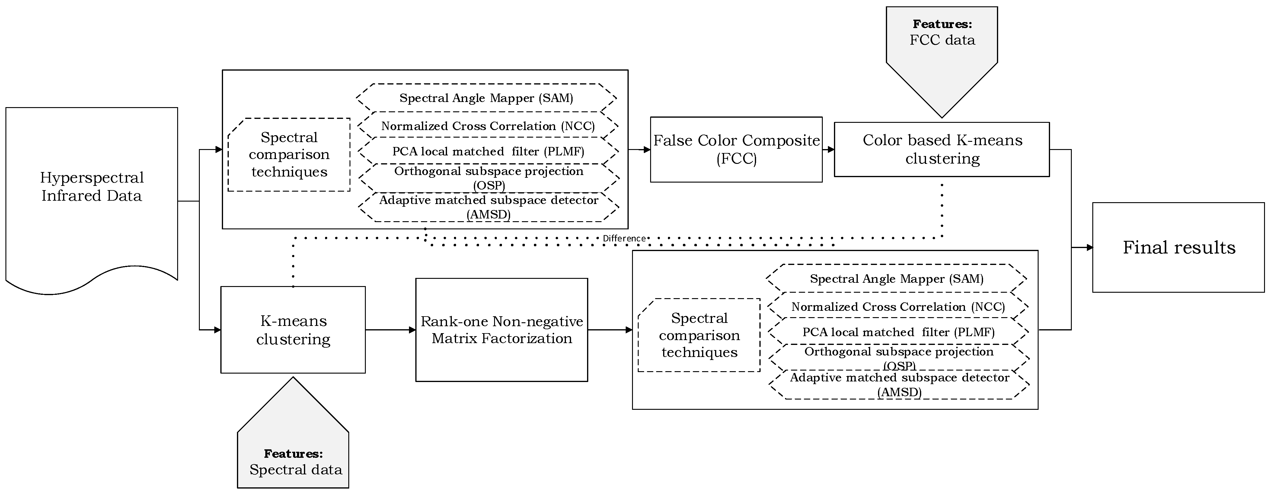
2.2. Clustering and Proposed Algorithms

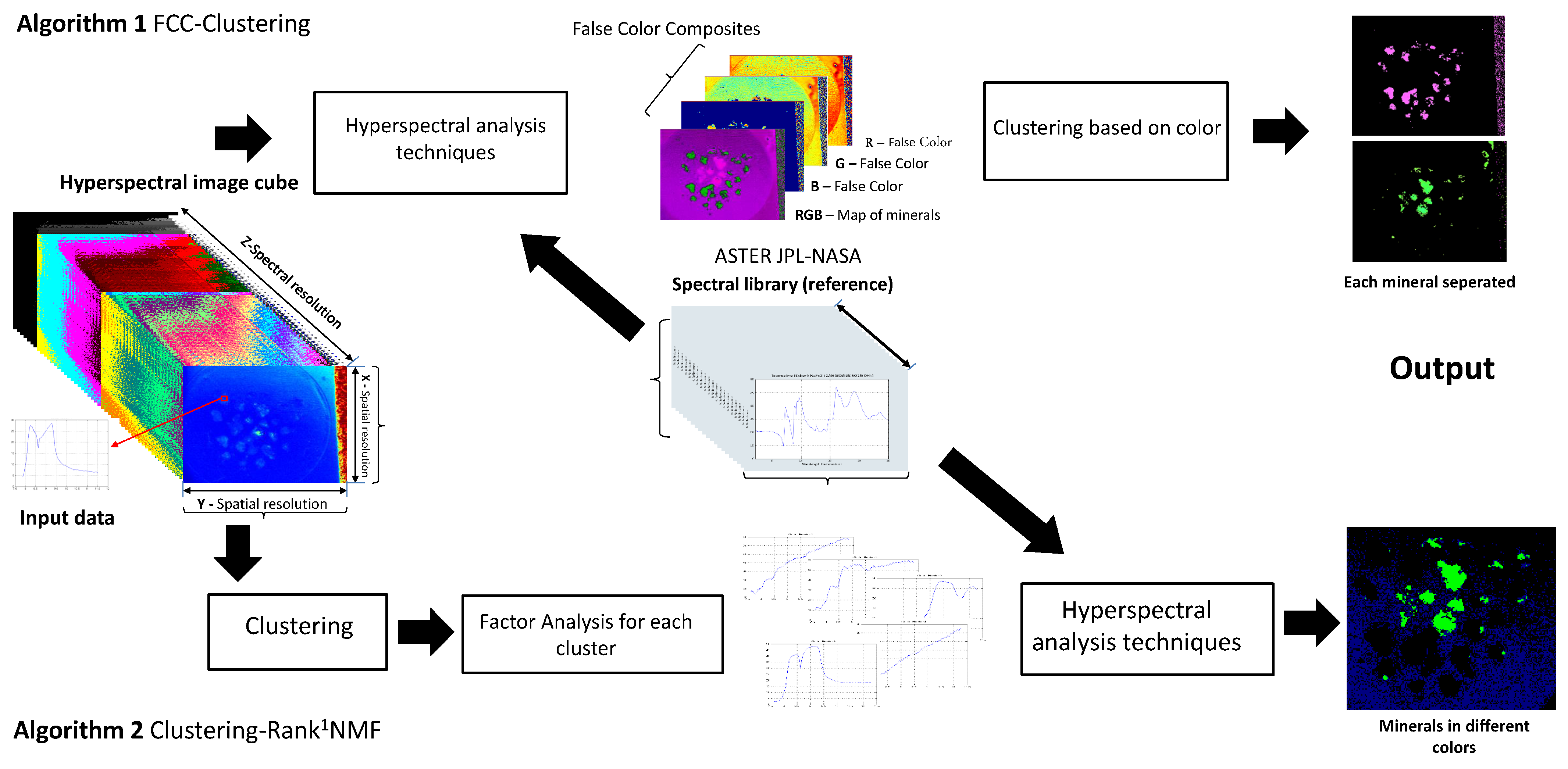
Clustering is a term used for an unsupervised learning approach (unlike classification, which is a supervised learning approach), to discriminate the spectra for the mineral identification in hyperspectral imagery. A clustering method provides a fast performance and reduces the typical difficulties of supervised approaches such as training and labeling that particularly occur when the number of mineral samples are limited [30]. The proposed approach applies the K-means clustering for both algorithms. However, the FCC-Clustering algorithm used HSV [76] (color) based clustering to group the RGB-FCC, and the clustering-rank${}^1$ NMF algorithm directly groups the spectra. FCC-clustering and clustering-rank${}^1$ NMF algorithms are presented in

Table 2. The FCC-clustering algorithm works by applying the clustering of false colors.

FCC-K-Means ALGORITHM
Given	Input data $\mathbf{I}(\mathit{x},\mathit{y},\mathit{z})\in R^{N\times M\times Z}$ is a continuum removed
	spectral data where $I(\mathit{x},\mathit{y})\in R^{N\times M}$ is the spatial dimension
	for RoI (in pixel unit), $\mathit{z}$ is the spectral resolution.
Step 1	Calculation of the spectral comparison techniques:
	$M_j(x,y)=S{T}_j(I(x,y),{\mathsf{\Phi }}_i)$
	$S{T}_j$ represents the spectral techniques corresponding to $\mathit{j}$
	(e.g., $j=1\to M_1=NCC$). ${\mathsf{\Phi }}_i\in R^z$ denotes the reference
	spectra (i.e., ASTER/JPL) with targeted mineral $\mathit{i}$.
Step 2	Generating FCC, ${\mathsf{\Psi }}_{RGB},$ using $M_j$ (for every $\mathit{j}$)
	applying thresholding.
Step 3	Let ${\mathsf{\Psi }}_{HSV}$ a representation of FCC in HSV color system,
	${\mathsf{\Psi }}_{HSV}(x,y,3)={\mathsf{\Psi }}_{RGB}(x,y,3).$ K-means method Clusters
	${\mathsf{\Psi }}_{HSV}(p,3),p\in R^{N\times M}$ into k categories.
	$J_k={\sum }_{k=1}^K{\sum }_{i=1}^3$$\parallel {\mathsf{\Psi }}_{HSV}{}_i-{\overline{\mathsf{\Psi }}}_k{\parallel }_2^2$
Output	$J_k$ represents the segmented mineral grains in different color.

and

Table 3. The clustering-rank${}^1$ NMF algorithm for directly grouping the spectra.

K-Means-Rank${}^1$ NMF ALGORITHM
Given	Input data $\mathbf{I}(\mathit{x},\mathit{y},\mathit{z})\in R^{N\times M\times Z}$ is a continuum removed
	spectral data where $I(\mathit{x},\mathit{y})\in R^{N\times M}$ is the spatial dimension
	for RoI (in pixel unit), $\mathit{z}$ is the spectral resolution.
Step 1	Clustering $X(p,z),p\in R^{N\times M}$ into k categories. The clustering
	is based on the spectral difference among the clusters (0 ≤ J ≤ k).
	$J_k={\sum }_{k=1}^K{\sum }_{C\left(i\right)=k}\parallel X_i-{\overline{X}}_k{\parallel }_2^2$
Step 2	$h_1^q$ is the rank one NMF (i = 1) of each cluster $C_i^q$ after clustering
	application.
	$\forall q|1<q<k,C_i^q=W\times h_i,i=1\Rightarrow h_1^q,q=1,\dots ,k$
Step 3	Calculate spectral comparison techniques:
	$M_j(x,y)=S{T}_j(h_1^q,{\mathsf{\Phi }}_i)$
	$S{T}_j$ represents the spectral techniques corresponding to $\mathit{j}$
	(e.g., $j=1\to M_1=NCC$). ${\mathsf{\Phi }}_i\in R^z$ denotes the reference
	spectra (i.e., ASTER/JPL) with targeted mineral $\mathit{i}$.
Output	Generating FCC, ${\mathsf{\Psi }}_{RGB},$ using $M_j$ (for every $\mathit{j}$)
	through thresholding.

, respectively. The spectral comparison techniques used in these two algorithms are referred to as $M_j(x,y)$, and it changes for comparison assessment in both algorithms following different techniques used for comparison assessment.

Parameters involved in the clustering in the proposed approach:

(1) The main concern to use the clustering algorithm involves the initial number of the clusters. Here, this number strictly depends on the number of targeted minerals. In addition, there are several ways to perform clustering without initialization cluster number (e.g., Elbow method [77]) that is far from the subject of this manuscript.

(2) In the case of direct clustering of spectra, the hyperspectral acquisition parameters were fixed for all samples (and remained unchanged) to have no variation in the grouping result.

2.3. FCC-Clustering

The FCC-Clustering algorithm is presented in Table 2. The input data of the algorithm, $I(x,y,z)\in R^{N\times M\times Z}$, is continuum removed spectral data [78,79] where $I(x,y)\in R^{N\times M}$ is the spatial dimension for selected RoI (contains targeted pixels), and z is the spectral resolution. Calculation of the spectral comparison techniques is shown by the following formulation:

$$M_j(x,y)=S{T}_j(I_j(x,y),{\mathsf{\Phi }}_i).$$

(6)

$S{T}_j$ represents the spectral techniques and j reveals the number of techniques exploited (e.g., $j=1⟶M_1=NCC$). ${\mathsf{\Phi }}_i\in R^z$ denotes the reference spectra (i.e., ASTER/JPL) and i is the number of spectra corresponds to number of targeted minerals. The generation of FCC, ${\mathsf{\Psi }}_{RGB}$, depends on the amount of $M_j$ (for every j). The three lowest $M_j$ create the (R,G,B) applying thresholding criterion. The output will be ${\mathsf{\Psi }}_{RGB}$, an image where the materials have been marked by different colors. Let ${\mathsf{\Psi }}_{HSV}$ be a representation of FCC in the HSV color system, ${\mathsf{\Psi }}_{HSV}(x,y,3)={\mathsf{\Psi }}_{RGB}(x,y,3)$. Clustering method groups ${\mathsf{\Psi }}_{HSV}(p,3),p\in R^{N\times M}$ into k categories. Here, a K-means clustering technique has been used; hence, we have:

$$J_k=\sum _{k=1}^K\sum _{i=1}^3\left|\right|{\mathsf{\Psi }}_{HS{V}_i}-{\overline{\mathsf{\Psi }}}_k{\left|\right|}_2^2$$

(7)

where $J_k$ represents the targeted mineral grains clustered from other minerals by different colors:

$$J_k=\sum _{k=1}^K\sum _{i=1}^3\left|\right|X_i-{\overline{X}}_k{\left|\right|}_2^2$$

(8)

2.4. Clustering-Rank${}^1$ NMF

In the Clustering-rank${}^1$, the NMF algorithm is presented in Table 3. The input data of the algorithm, $I(x,y,z)\in R^{N\times M\times Z}$, is continuum removed spectral data where $I(x,y)\in R^{N\times M}$ is the spatial dimension for selected RoI (contains targeted pixels), and z is the spectral resolution. Clustering $x(p,z),p\in R^{N\times M}$ into k categories, the clustering is based on the spectral difference among the clusters ($0\le J\le k$):

$$J_k=\sum _{k=1}^K\sum _{c\left(i\right)=k}\left|\right|X_i-{\overline{X}}_k{\left|\right|}_2^2$$

(9)

$h_1^q$ is the rank one NMF ($i=1$) of each cluster $C_i^q$ after clustering application; $\forall q|1<q<k,C_i^q=W\times h_i,i=1\Rightarrow h_1^q,q=1,...,k$. Calculation of the spectral comparison techniques is as follows:

$$M_j(x,y)=S{T}_j(h_1^q,{\mathsf{\Phi }}_i)$$

(10)

$S{T}_j$ represents the spectral techniques and j reveals the number of techniques exploited (e.g., $j=1⟶M_1=NCC$SAM). ${\mathsf{\Phi }}_i\in R^z$ denotes the reference spectra (i.e., ASTER/JPL) and i is the number of spectra that corresponds to the number of targeted minerals. The generation of FCC, ${\mathsf{\Psi }}_{RGB}$, depends on the amount of $M_j$ (for every j). By thresholding, the three lowest $M_j$ create $(R,G,B)$. The output will be ${\mathsf{\Psi }}_{RGB}$, an image where the materials have been marked by different colors.

2.5. Accuracy of the Proposed Approach

The accuracy of the algorithms is based on counting the correct detected pixels in the hyperspectral images (

Table 4. The quantitative accuracy of the two algorithms.

Accuracy
		Rigid GT		FCC-Clustering		Rank${}^{\mathbf{1}}$ NMF
Mineral	Spatial Resolution			NCC	SAM	NCC	SAM
		Mineral	Quartz	Acc (%)	Acc (%)	Acc (%)	Acc (%)
Biotite	123 × 138	496	885	52.45	68.79	78.58	78.58
Diopside	126 × 143	299	888	40.21	71.59	70.17	59.906
Epidote	123 × 148	260	890	48.64	70.54	81.66	81.66
Geothite	118 × 141	235	718	33.76	64.36	55.94	55.94
Kyanite	123 × 144	88	659	37.44	69.54	81.48	81.48
Scheelite	123 × 158	168	1006	48.69	56.51	84.87	59.29
Smithsonite	119 × 160	402	1117	28.39	47.24	50.91	67.15
Tourmaline	58 × 80	122	14	75.81	49.73	57.77	68.08
Pyrope	159 × 159	259	1654	<1	8.67	61.07	11.63
Olivine	172 × 142	435	2649	6.53	18.49	<1	7.028

and

Table 5. The computational time of the two algorithms.

	Computational Time (s)
		FCC-Clustering											Rank${}^{\mathbf{1}}$ NMF Algorithm
Minerals						MF					RoI						MF
	RoI	NCC	SAM	OSP	AMSD			RMF				NCC		SAM	OSP	AMSD			RMF
							PLMF											PLMF
								Sum	μLocal	μGlobal									Sum	μLocal	μGlobal
Biotite	131 × 143	310.39	273.74	808.21	865.07	609.35	376.20	376.36	383.67	377.87	123 × 141	15.25		15.23	15.63	15.69	15.36	15.20	15.19	15.20	15.63
Diopside	128 × 145	288.62	254.89	717.27	792.97	619.64	421.45	447.48	405.89	380.92	124 × 125	14.78		14.76	15.23	15.02	14.89	14.74	14.73	14.74	15.23
Epidote	125 × 157	332.82	320.90	863.70	907.06	608.15	433.59	440.40	459.21	468.72	125 × 157	22.12		22.11	22.49	23.1	22.23	22.08	22.08	22.08	22.49
Geothite	124 × 144	298.09	261.75	751.28	794.36	545.00	374.33	374.12	381.94	376.25	120 × 149	21.72		21.69	22.06	23.18	21.81	21.67	21.67	21.69	22.07
Kyanite	129 × 144	304.68	264.29	609.55	657.05	609.36	487.18	664.28	394.87	386.91	126 × 147	24.34		24.33	24.74	24.89	24.46	24.31	24.31	24.31	24.74
Scheelite	136 × 172	514.34	462.17	834.13	886.73	846.71	582.24	621.27	658.24	634.79	125 × 160	22.99		22.96	23.36	23.92	23.07	22.95	22.95	22.94	23.36
Smithsonite	120 × 163	384.92	293.94	783.89	826.86	641.74	409.60	411.54	417.70	410.70	119 × 160	22.37		22.35	22.89	23.51	22.51	22.35	22.35	22.34	22.88
Tourmaline	50 × 55	211.01	205.60	269.15	289.13	252.78	213.70	213.57	214.16	213.51	56 × 62	7.79		7.78	8.12	8.83	7.89	7.75	7.75	7.75	8.12
Pyrope	144 × 152	362.38	325.40	674.05	693.06	652.95	349.78	346.04	356.81	347.67	159 × 170	18.75		18.73	19.14	19.94	18.83	18.70	18.70	18.70	19.14
Olivine	157 × 139	497.70	331.28	1.0067 ×10${}^3$	841.98	627.43	7.8214 × 10${}^3$	369.47	356.42	1.2252 × 10${}^3$	159 × 173	22.14		22.11	22.58	23.27	22.21	22.07	22.07	22.06	22.58

). For that, a ground truth is used following the rigid manual labeling of the known location of the mineral grains in the samples and verified by the results of μX-ray fluorescence (μXRF (Figure 3). The number of ground truth pixels in each cases is also mentioned for all the samples with spatial resolution of ROI. For every case of mineral mixture, the targeted mineral grains are mixed with quartz grains; hence, for each mixed sample, accuracy is estimated through the accuracy of discrimination between these two types of grains. Two types of errors are shown by false positives that represent wrong mineral identification (one mineral instead of other) and a false negative that reveals misidentification of the mineral grains, and both are calculated in each case. Total accuracy of each algorithm is calculated by subtraction of the correct identification and two errors for every sample:

$$Totalaccuracy=ACC(\%)-FN(\%)-FP(\%)$$

(11)

where local accuracy ($ACC$) is calculated by:

$$ACC(\%)=\frac{Correctdetectedpixels}{Totalpixelsofmineral\left(ROI\right)}*100$$

(12)

Let $FN$ stands for the false negative error and estimate it using below mentioned formulas:

$$FN(\%)=\frac{TotalROI-Correctdetectedpixels}{TotalROI}*100$$

(13)

The False Positive ($FP$) error is the wrong classified pixels and calculates by:

$$FP(\%)=\frac{Wrongclassifiedpixels}{TotalROI}*100$$

(14)

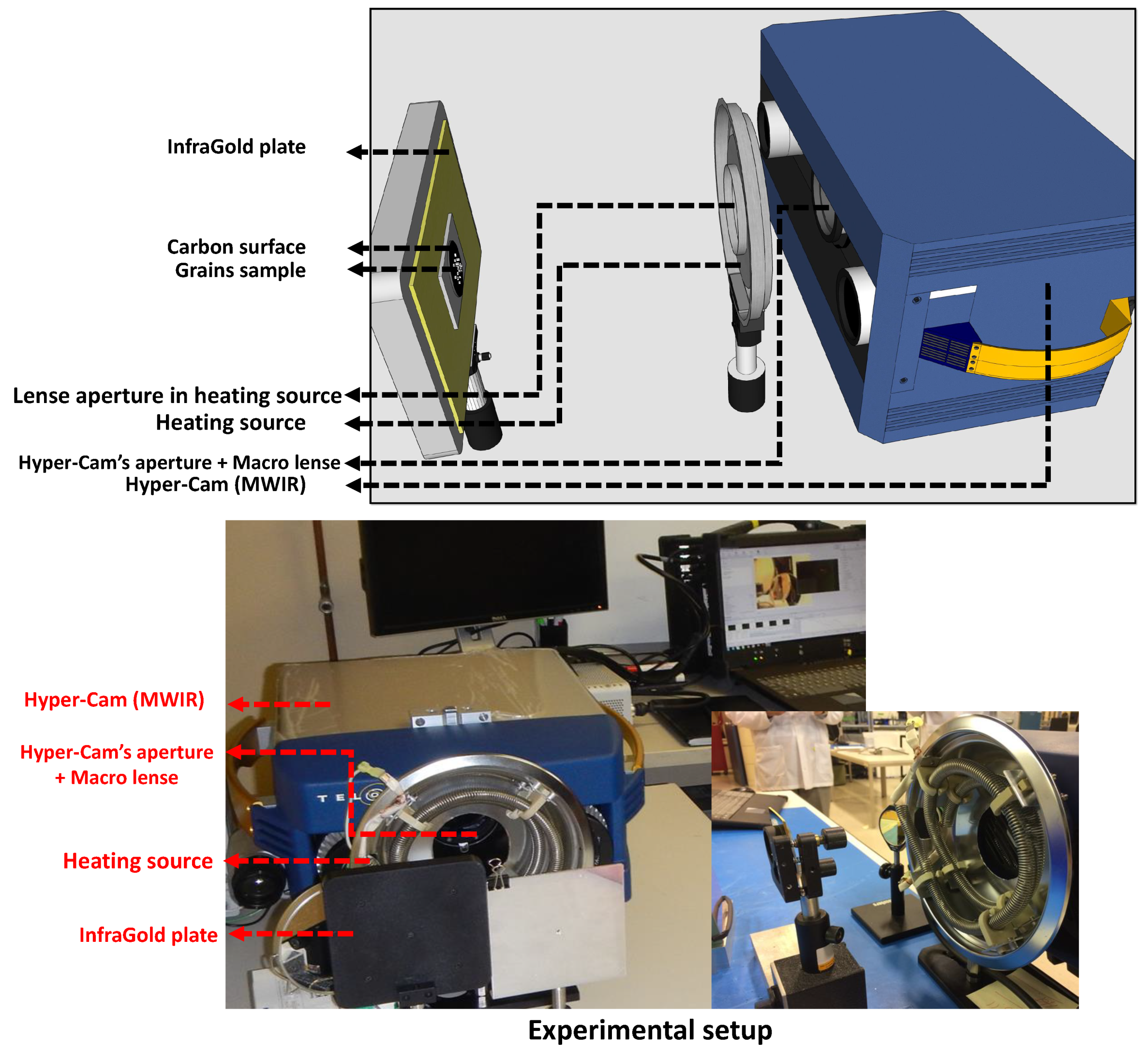
3. Mineral Grains and Experimental Set Up

The experiment was conducted in a laboratory environment with a lightweight Hyper-Camera imaging spectroradiometer (HYPER-CAM LW) [80] operating in the long-wave infrared (LWIR) band (from 7.7 to 11.8 μm). It has spatial resolution of $320\times 256$ with a LWIR PV-MCT focal plane array detector. It has a spectral resolution of 4 cm${}^{-1}$ which gives the spectra from 868 to 1270 cm${}^{-1}$. The individual spectra are gathered using the Fourier-Transform Infrared Spectrometer (FT-IR) for every pixel with an instantaneous field-of-view of 0.35 mrad [80]. There is a heating source between the hyperspectral camera, and the grain samples (Figure 4 depict the experimental setup) to closely and uniformly radiate the samples. Having the heating source located to the side of the sample and the camera enables radiating the heat more uniformly. There are eight mineral grains targeted to be automatically identified using the spectral analysis. Figure 5 shows the spectra from mineral grains used in the experiments together with the spectra from ASTER JPL-NASA spectral library to demonstrate the qualitative similarity among experimental and reference spectra. A brief description of targeted minerals is presented in

Table 6. Characteristic of minerals studied by LWIR.

Minerals	Chemical Formula
Biotite	$K{(Mg,Fe)}_{2-3}A{l}_{1-2}S{i}_{2-3}{O}_{10}{(OH,F)}_2$
Diopside	$MgCaS{i}_2{O}_6$
Epidote	$C{a}_2(A{l}_2,Fe)\left(Si{O}_4\right)\left(S{i}_2{O}_7\right)O\left(OH\right)$
Goethite	(FeO(OH))
Kyanite	$A{l}_{2}Si{O}_5$
Scheelite	$CaW{O}_4$
Smithsonite	$\left(ZnC{O}_3\right)$
Tourmaline	$\left((Na,Ca){(Mg,Li,Al,F{e}^{2+})}_{3}A{l}_6{\left(B{O}_3\right)}_{3}S{i}_6{O}_{18}{\left(OH\right)}_4\right)$
Olivine	${(M{g}^{+2},F{e}^{+2})}_{2}Si{O}_4$
Pyrope	$M{g}_{3}A{l}_2{\left(Si{O}_4\right)}_3$
Quartz	$Si{O}_2$

.

Properties of Hyperspectral Image

The image acquisitions have been performed while the minerals were attached to a carbon substrate (shown in Figure 3a–e) and had an infragold plate in the background. The infragold plate reflects all the radiation and is used to calculate the overall radiation’s amount for Continuum Removal (CR) [78]. The experiment was performed while the heating source was first on and then off. It is required to perform CR and avoid calculation of the black-body’s temperature [78,79]. The size of hyperspectral images is $180\times 300$ pixels in the spatial resolution and 122 channels of spectral resolution.

Mineral identification using hyperspectral technology depends on spectral comparison techniques and mineral spectral signature. The spectra for some of these minerals (e.g., Figure 5) are represented by maximum or minimum in particular wavelength. The location and types of these particular features within the wavelength band play an important role in the identification’s accuracy. The minerals for this research have reasonable signatures in the 7.7–11.8 μm band. Smithsonite, scheelite, and goethite have more similar spectra to each other in terms of spectral shape (location of extrema). This causes a problem for identification of the minerals once they are combined in a mixture form as their spectral features would be similar. In this example, only scheelite has a maximum peak before 11.8 μm, and it makes scheelite detectable. In contrast, goethite and smithsonite have a peak after a 11.8 μm band (not in the range of our hyper-camera), and this makes them undetectable for both algorithms (geothite example in Figure 3c and Figure 5) with the used system.

4. Results

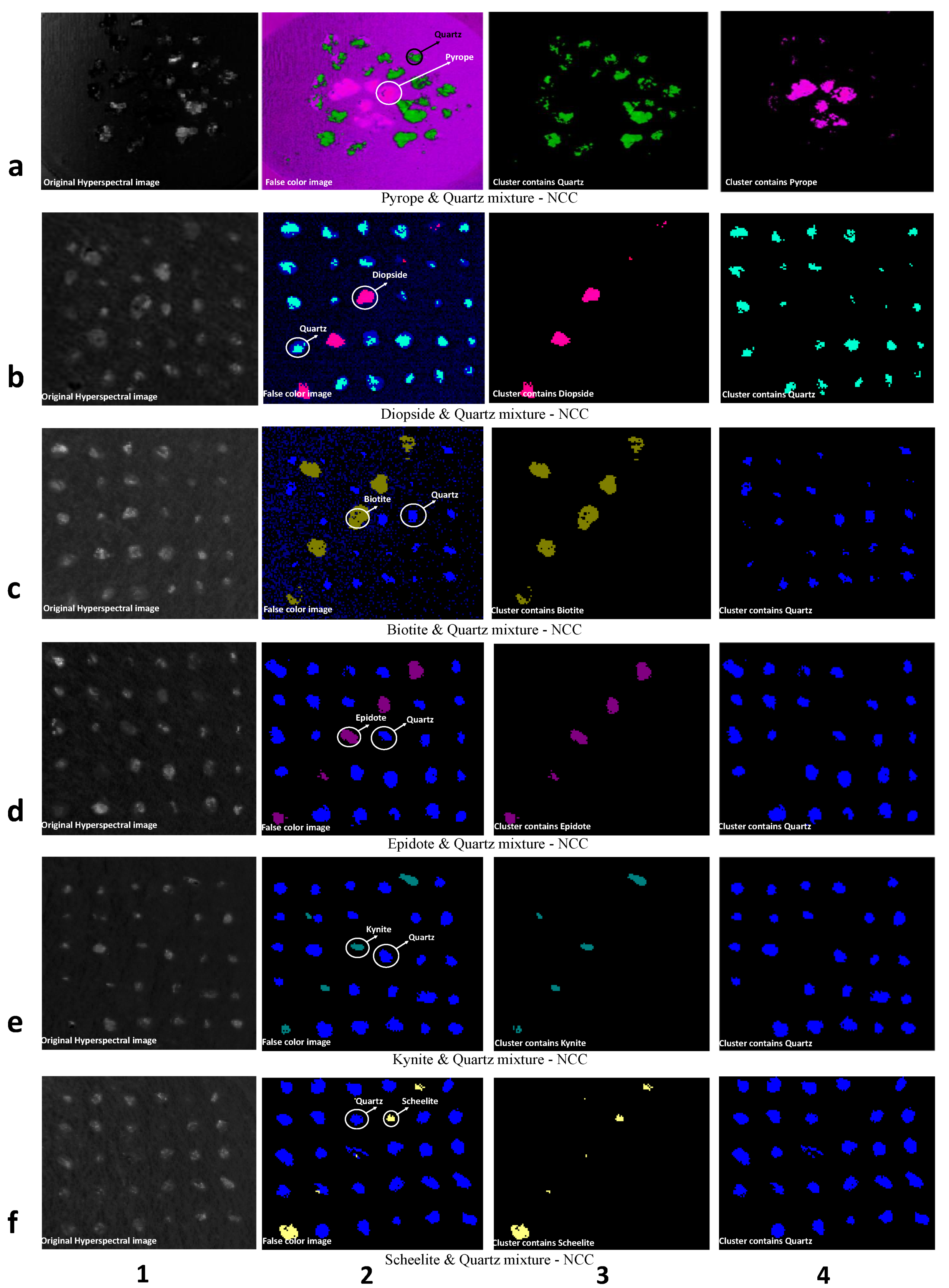
4.1. The Results of Spectral Comparison Techniques

The results are shown for the FCC-clustering proposed algorithm using the RGB-FCC (Figure 5 and Figure 6). This provides a better visualization of the spectral differences among the minerals by placing each mineral target as a certain weight amount in colors. FCC provides a good difference criterion that can easily be discriminated by a clustering approach (the results of the FCC-clustering algorithm are shown in Figure 6). Some of the spectral techniques applied to the images are not necessarily for spectral comparison approaches such as NCC or SAM. However, these techniques have been used to investigate the strength of the method with respect to the extraction of spectral differences. In order to apply these techniques, a MATLAB hyperspectral image index analysis toolbox [81] was used. The quantitative results of the FCC-clustering algorithm are shown in Table 2.

4.2. Results of the Two Algorithms

The results of the spectral comparison technique were presented in the previous section; in this section, the clustering results are shown in Figure 5 and Figure 6. This includes the clustering approach for both algorithms. The results of the FCC-clustering strategy are presented in comparison with the second hyperspectral method. Applying the clustering in a different hierarchy with spectral analysis techniques creates two approaches that have two similar outcomes. Figure 6 shows the performance of the color based clustering approach for the algorithms. Besides the computational load which is considered as significantly different between these methods (Table 5), clustering after using spectral analysis (in the FCC-clustering algorithm) is considered as a more sensitive algorithm, and this is caused by the dependency of the clustering to the generated color (RGB-FCC). A low performance in spectral comparison techniques creates misclassification in the algorithm, for instance: diopside applying NCC has lower performance than SAM, and it created more false negatives after clustering (Table 2).

However, the sensitivity of the clustering-rank${}^1$ NMF algorithm lies under the application of clustering techniques. The same example of diopside that has more false negatives because of clustering poor performance (Table 4). Sometimes, due to the spectral curve that does not have significant extrema in the band of the hyperspectral information, the clustering method cannot discriminate the clusters from each other (i.e., in the case of goethite and smithsonite minerals). In such a situation, increasing the number of groups in the clustering initialization partially solves the problem. Even though this solves the problem in the clustering, the clusters selected as different categories might have similar content materials. This is corrected by the application of the spectral comparison techniques that categorize all of this similar grouping into one category. However, in the case of similar mineral spectra or unspecified spectral exterma in minerals, the problem remains unsolved.

Applying these algorithms provides an opportunity to compare them through the mineral identification task and resulting computational load. The FCC-clustering algorithm seems heavier in computation time when compared to the clustering-rank${}^1$ NMF algorithm due to the application of the spectral analysis for each spectrum. Furthermore, the clustering-rank${}^1$ NMF algorithm clusters all the spectra that result in heavy computations as well. Table 4 presents the accuracy of both algorithms, and Table 5 indicates the computational load for each algorithm with different spectral analysis. Averaging and factor analysis can provide better outcomes, particularly the factor analysis provides more statistical information for the selection of the spectral representative in the algorithm. We applied NMF to select a spectral representative for each cluster. Figure 5 and Figure 7 show some examples of NMF results and box-plots for different categories of minerals and present the qualitative and quantitative representation for the application of such techniques, respectively. A higher number of initialization for the clustering allows a re-selection of the same spectral mineral in two or more different categories. This difficulty can also be solved in the latter hierarchy by applying spectral analysis, which means that this analysis selects the same mineral categories for these selections.

It is noticeable that the location of the detected pixels is vital to identify the mineral grains. In other words, we would like to have correctly detected pixels located on the surface of mineral grains and even one or two pixels detected on the surface of minerals indicate the grain content and ultimately could yield to an accurate identification (grain-based identification). We also provide pixel-based accuracy percentages (at Table 4 or

Table 7. The quantitative accuracy for spectral comparison techniques in the second algorithm.

Accuracy of Spectral Comparison Techniques
Minerals Mixture	NCC (%)			SAM (%)			OSP (%)			AMSD (%)
	ACC	FN	FP	ACC	FN	FP	ACC	FN	FP	ACC	FN	FP
Biotite & Quartz	96.81	14.85	3.37	96.81	14.85	3.37	55.43	34.94	0.84	77.52	11.93	4.11
Diopside & Quartz	87.02	13.67	3.18	82.42	4.33	18.18	80.57	52.61	1.87	71.25	26.05	1.08
Epidote & Quartz	92.01	6.99	3.36	92.01	6.99	3.36	97.14	34.38	7.12	79.49	21.59	4.83
Geothite & Quartz	80.86	21.77	3.15	80.86	21.77	3.15	79.01	55.36	1.25	67.39	17.66	1.92
Kyanite & Quartz	90.86	5.66	3.72	90.86	5.66	3.72	71.84	24.30	1.39	86.29	6.01	7.04
Scheelite & Quartz	96.60	7.58	4.19	81.24	2.30	19.64	95.76	30.19	1.43	90.25	8.49	2.51
Smithsonite & Quartz	78.72	23.96	0	93.96	21.50	5.31	69.85	37.07	1.44	66.37	31.96	0.98
Tourmaline & Quartz	73.76	12.96	4.31	86.28	15.16	3.03	75.32	22.55	2.26	86.24	21.56	2.36
Pyrope & Quartz	72.13	4.28	6.78	81.74	0.68	69.43	86.83	12.54	2.07	51.08	6.65	5.17
Olivine & Quartz	62.69	60.83	1.42	84.78	5.85	71.90	83.96	5.57	3.64	73.17	10.67	8.88

). For example, kyanite and scheelite have been detected with a very limited number of pixels but very accurately because these pixels are in the grain’s surface. In terms of spectral comparison technique accuracy of the algorithms, the SAM and NCC provided better accuracy as compared to OSA and AMSD that required the background spectra in their calculations. Matching filter (PLMF) did not succeed with detecting the minerals and was omitted from the accuracy calculations. Table 4 shows the accuracy of spectral comparison techniques using the clustering-rank${}^1$ NMF algorithm. The accuracy of biotite & quartz, epidote and quartz, geothite and quartz, and kyanite and quartz are the same for NCC and SAM, and this indicates the dependency of the clustering-rank${}^1$ NMF algorithm to the clustering. This is also shown in Table 3 for the clustering-rank${}^1$ NMF algorithm. However, the accuracy of NCC and SAM in the FCC-clustering algorithm is not similar and indicates that the identification process in the FCC-clustering algorithm depends more on the performance of the spectral comparison techniques than on clustering.

5. Discussion

5.1. Automatic Identification Process

Mineral identification has been studied and researched for several decades, and most of these approaches have been categorized under the hyperspectral remote sensing, airborne, portable instruments [82], and core logging [83] applications. The proposed research addressed the application of hyperspectral infrared in the LWIR (7.7–11.8 μm) for the purpose of automated mineral identification applying two algorithms that involved unsupervised segmentation and spectral comparison techniques. It has been previously shown that clustering techniques are more suitable for categorizing the minerals as compared to classification (supervised) approaches. This is because of not having enough data to properly train the classifier and expensive labeling [30,78]. Applying spectral comparison techniques and clustering approaches gave the opportunity to identify the minerals using two algorithms. The difference between these two approaches lies in the utilization of these techniques in different hierarchies. Applying clustering or spectral comparison approaches for all data spectral points in these two algorithms is considered as the bottle neck for both algorithms due to the categorization task. Each of these algorithms, for all the data points, can lead the entire algorithm to a high or low computational complexity. The algorithms have reasonable performance for the identification of the minerals. Some minerals such as goethite and smithsonite have no specific extrema in their LWIR spectra and their identification failed, regardless of which algorithm is applied (it is shown in Figure 5 and also Table 4). In contrast, biotite, diopside, epidote, tourmaline, scheelite, quartz, and kyanite have been identified more clearly due to their distinctive spectral signature in the LWIR.

5.2. Computational Complexity of the Algorithms

We analyzed two different algorithms using spectral comparison and clustering techniques applied in different hierarchies. The FCC-clustering algorithm calculates the spectral techniques for all the pixels of hyperspectral image spectra and gave false colors to these features and ultimately segmented these false color regions by applying clustering. On the contrary, the clustering-rank${}^1$ NMF algorithm directly applies the clustering to all the pixels in the hyperspectral image. Then, the first rank of NMF is selected as the spectral representative for each cluster (the statistical relationship among the clusters are shown by box-plots in Figure 7). These spectra were compared with the reference spectra (ASTER spectral library) and this led to finalizing the segmentation process. Selecting the representative of each group using low-rank NMF (here rank-¹ NMF) from each group alleviates the influence of miss-classification (occurred by clustering) in the final spectral comparison ([79,84] and showed that averaging of spectra would not be effective as far as decomposition/factorization methods work). Moreover, NMF shows better performance than the PCA, which might suffer from sensitivity to outliers and noise).

The FCC-clustering algorithm shows itself to be more computationally costly as compared to the clustering-rank${}^1$ NMF algorithm because of the application of the spectral comparison approaches to the entire pixel’s spectra of the hyperspectral images. Nevertheless, the results presented in Table 4 indicate that the clustering-rank${}^1$ NMF algorithm is also computationally costly due to direct clustering for the whole spectral pixel points. The computational complexity of the clustering (here K-means) algorithm for the fixed k and d (dimension) is $O\left(n^{(dk+1)}\log n\right)$, where n is the number of entities to be clustered [85]. Some heuristic algorithms such as Lloyds algorithm have the complexity of $O\left(nkdi\right)$, where k is the number of clusters, i is the number of iteration, and n is the number of d-dimensional vectors [86]. On the other hand, some algorithms such as SAM have a cosine function and have approximately a computational complexity of cosine which is $O\left(M\right(n\left)\log n\right)$ (for the algorithm of Arithmetic-geometric mean iteration), where $M\left(n\right)$ stands for the chosen multiplication algorithm complexity [87]. Due to the division into the cosine function in the SAM, the complexity of $O\left(n^2\right)$ corresponds to the division itself which increases the whole complexity of the SAM function. The different computational complexity between clustering and spectral comparison techniques is the reason why calculation of the spectra for the clustering-rank${}^1$ NMF algorithm shows considerably lower complexity as compared to the FCC-clustering algorithm.

The sensitivity of each algorithm depends on the spectral difference calculations. For example, the FCC-clustering algorithm is sensitive to spectral techniques used for extraction of the RGB-FCC to finally clustering them. However, there are many other better alternative approaches that exist for visualization of spectra in the hyperspectral imagery (i.e., [88,89,90,91]) that can replace the current FCC method. In the clustering-rank${}^1$ NMF algorithm, the sensitivity of the system lies in the clustering approach and, in particular, the number of initialization in clustering. Besides this, there are other factors nominally involved in the sensitivity of the proposed approaches such as the initialization of the clustering for the FCC-clustering approach and the spectral analysis in the clustering-rank${}^1$ NMF method. In the clustering-rank${}^1$ NMF algorithm, a spectrum from each selected cluster should be compared to reference spectra from the ASTER JPL-NASA spectral library. Several methods can be applied to select the best representative spectrum from each cluster such as randomly selecting one spectrum, spectral averaging, or using factor analysis. Random or averaging selection of the spectrum might not be an efficient way to select the spectral representative in each cluster because of averaging and random calculation sensitivity against bad spectra (wrongly grouped spectra or noisy spectra) that may occur in the process. Some noisy spectra might be clustered into the different category of minerals and random (or averaging) selection may not be a good option to suppress this effect, and this ultimately influences the mineral identification.

6. Conclusions

The proposed approach presented a geological hyperspectral infrared imagery (in the 7.7–11.8 μm-LWIR range) in laboratory conditions. This paper addressed quantitative and qualitative assessments of two algorithms for the identification of several minerals and challenged the application of clustering. The FCC-clustering algorithm applied the spectral comparison techniques on the entire pixel-spectra of the input data cube and spectral library of JPL/NASA. It generated the spectral difference that was presented in RGB-FCC form, and a clustering grouped the different composites. The clustering-rank${}^1$ NMF algorithm clustered all the pixel-spectra into different categories. Then, rank${}^1$ extracted from NMF as representative for each cluster were compared to the spectral library of JPL/NASA through spectral comparison techniques that generated RGB-FCC results. The results of the clustering-rank${}^1$ NMF algorithm indicated more significant computational efficiency (more than 20 times faster) than the FCC-clustering algorithm. The clustering-rank${}^1$ NMF algorithm showed more dependency on clustering rather than the FCC-clustering algorithm that was more sensitive to spectral comparison techniques. Both algorithms had promising performance for mineral identification having even more than 90% accuracy (using) a clustering-rank${}^1$ NMF algorithm. Several spectral techniques were used such as AMSD, OSP, PLMF, SAM, and NCC, but most of them showed a similar accuracy range (although PLMF exhibited a lower accuracy). Eleven different mineral grains (biotite, diopside, epidote, goethite, kyanite, scheelite, smithsonite, tourmaline, pyrope, olivine, and quartz) were studied. Future work can be more focused on clustering approaches and the noise effect in mineral identification to increase the performance of the system. The study of minerals with poorly shaped spectra is another important future research avenue.

References

1. Kruse, F. Identification and mapping of minerals in drill core using hyperspectral image analysis of infrared reflectance spectra. Int. J. Remote Sens. 1996, 17, 1623–1632. [Google Scholar] [CrossRef]
2. Geotechnos. 2004. Available online: http://www.geotechnos.co.jp (accessed on 1 May 2021).
3. Yajima, T.; Ohkawa, K.; Huzikawa, S. Hyperspectral alteration mineral mapping using the POSAM method. In Proceedings of the 2004 IEEE International Geoscience and Remote Sensing Symposium (IGARSS 2004), Anchorage, AK, USA, 20–24 September 2004; Volume 2, pp. 1491–1493. [Google Scholar]
4. Huzikawa, S.; Ohkawa, K.; Tanaka, S. Automatic Identification of Alteration Mineral Using a Portable Infrared Spectralmeter. J. Remote Sens. Soc. Jpn. 2001, 21, 206–209. [Google Scholar]
5. Davis, C.O. Airborne Hyperspectral Remote Sensing; Technical Report; Naval Research Lab: Washington, DC, USA, 2001. [Google Scholar]
6. Goetz, A.F. Three decades of hyperspectral remote sensing of the Earth: A personal view. Remote Sens. Environ. 2009, 113, S5–S16. [Google Scholar] [CrossRef]
7. Zhang, L.; Zhang, L.; Tao, D.; Huang, X.; Du, B. Hyperspectral remote sensing image subpixel target detection based on supervised metric learning. IEEE Trans. Geosci. Remote Sens. 2014, 52, 4955–4965. [Google Scholar] [CrossRef]
8. Van der Meer, F.D.; Van der Werff, H.M.; Van Ruitenbeek, F.J.; Hecker, C.A.; Bakker, W.H.; Noomen, M.F.; Van Der Meijde, M.; Carranza, E.J.M.; De Smeth, J.B.; Woldai, T. Multi-and hyperspectral geologic remote sensing: A review. Int. J. Appl. Earth Obs. Geoinf. 2012, 14, 112–128. [Google Scholar] [CrossRef]
9. Boardman, J.W.; Kruse, F.A.; Green, R.O. Mapping Target Signatures via Partial Unmixing of AVIRIS Data; Jet Propulsion Laboratory NASA: Pasadena, CA, USA, 1995. [Google Scholar]
10. Herrmann, W.; Blake, M.; Doyle, M.; Huston, D.; Kamprad, J.; Merry, N.; Pontual, S. Short wavelength infrared (SWIR) spectral analysis of hydrothermal alteration zones associated with base metal sulfide deposits at Rosebery and Western Tharsis, Tasmania, and Highway-Reward, Queensland. Econ. Geol. 2001, 96, 939–955. [Google Scholar] [CrossRef]
11. Clark, R.N.; Swayze, G.A.; Livo, K.E.; Kokaly, R.F.; Sutley, S.J.; Dalton, J.B.; McDougal, R.R.; Gent, C.A. Imaging spectroscopy: Earth and planetary remote sensing with the USGS Tetracorder and expert systems. J. Geophys. Res. Planets 2003, 108. [Google Scholar] [CrossRef]
12. Liu, D.; Zhu, X. An enhanced physical method for downscaling thermal infrared radiance. IEEE Geosci. Remote Sens. Lett. 2012, 9, 690–694. [Google Scholar]
13. Kruse, F.; Lefkoff, A.; Boardman, J.; Heidebrecht, K.; Shapiro, A.; Barloon, P.; Goetz, A. The spectral image processing system (SIPS)—Interactive visualization and analysis of imaging spectrometer data. Remote Sens. Environ. 1993, 44, 145–163. [Google Scholar] [CrossRef]
14. Kruse, F.; Lefkoff, A.; Dietz, J. Expert system-based mineral mapping in northern Death Valley, California/Nevada, using the airborne visible/infrared imaging spectrometer (AVIRIS). Remote Sens. Environ. 1993, 44, 309–336. [Google Scholar] [CrossRef]
15. Boardman, J.W. Inversion of Imaging Spectrometry Data Using Singular Value Decomposition; IEEE: Vancouver, BC, Canada, 1989. [Google Scholar]
16. Boardman, J.W. Sedimentary facies analysis using imaging spectrometry. In Proceedings of the 8th Thematic Conference on Geologic Remote Sensing, Denver, CO, USA, 29 April–2 May 1991; Volume 2, pp. 1189–1199. [Google Scholar]
17. Center for the Study of Earth from Space (CSES). SIPS User’s Guide, Spectral Image Processing System; Version 1.2; Center for the Study of Earth from Space: Boulder, CO, USA, 1992; Volume 4, 88p. [Google Scholar]
18. Gillespie, A.R.; Kahle, A.B.; Walker, R.E. Color enhancement of highly correlated images. I. Decorrelation and HSI contrast stretches. Remote Sens. Environ. 1986, 20, 209–235. [Google Scholar] [CrossRef]
19. Gillespie, A.R.; Kahle, A.B.; Walker, R.E. Color enhancement of highly correlated images. II. Channel ratio and “chromaticity” transformation techniques. Remote Sens. Environ. 1987, 22, 343–365. [Google Scholar] [CrossRef]
20. Butt, M.J. Estimation of light pollution using satellite remote sensing and geographic information system techniques. GISci. Remote Sens. 2012, 49, 609–621. [Google Scholar] [CrossRef]
21. Tuia, D.; Camps-Valls, G. Urban image classification with semisupervised multiscale cluster kernels. IEEE J. Sel. Top. Appl. Earth Obs. Remote Sens. 2011, 4, 65–74. [Google Scholar] [CrossRef]
22. Dópido, I.; Villa, A.; Plaza, A.; Gamba, P. A quantitative and comparative assessment of unmixing-based feature extraction techniques for hyperspectral image classification. IEEE J. Sel. Top. Appl. Earth Obs. Remote Sens. 2012, 5, 421–435. [Google Scholar] [CrossRef]
23. Pompilio, L.; Pepe, M.; Pedrazzi, G.; Marinangeli, L. Informational clustering of hyperspectral data. IEEE J. Sel. Top. Appl. Earth Obs. Remote Sens. 2014, 7, 2209–2223. [Google Scholar] [CrossRef]
24. Izquierdo-Verdiguier, E.; Gomez-Chova, L.; Bruzzone, L.; Camps-Valls, G. Semisupervised kernel feature extraction for remote sensing image analysis. IEEE Trans. Geosci. Remote Sens. 2014, 52, 5567–5578. [Google Scholar] [CrossRef]
25. Khodadadzadeh, M.; Li, J.; Plaza, A.; Bioucas-Dias, J.M. A subspace-based multinomial logistic regression for hyperspectral image classification. IEEE Geosci. Remote Sens. Lett. 2014, 11, 2105–2109. [Google Scholar] [CrossRef]
26. De Boissieu, F.; Sevin, B.; Cudahy, T.; Mangeas, M.; Chevrel, S.; Ong, C.; Rodger, A.; Maurizot, P.; Laukamp, C.; Lau, I.; et al. Regolith-geology mapping with support vector machine: A case study over weathered Ni-bearing peridotites, New Caledonia. Int. J. Appl. Earth Obs. Geoinf. 2018, 64, 377–385. [Google Scholar] [CrossRef]
27. Shao, Z.; Zhang, L.; Zhou, X.; Ding, L. A novel hierarchical semisupervised SVM for classification of hyperspectral images. IEEE Geosci. Remote Sens. Lett. 2014, 11, 1609–1613. [Google Scholar] [CrossRef]
28. Zhang, L.; Zhang, L.; Du, B. Deep learning for remote sensing data: A technical tutorial on the state of the art. IEEE Geosci. Remote Sens. Mag. 2016, 4, 22–40. [Google Scholar] [CrossRef]
29. Chen, Y.; Nasrabadi, N.M.; Tran, T.D. Hyperspectral image classification via kernel sparse representation. IEEE Trans. Geosci. Remote Sens. 2013, 51, 217–231. [Google Scholar] [CrossRef] [Green Version]
30. Yousefi, B.; Sojasi, S.; Castanedo, C.I.; Beaudoin, G.; Huot, F.; Maldague, X.P.; Chamberland, M.; Lalonde, E. Mineral identification in hyperspectral imaging using Sparse-PCA. In Thermosense: Thermal Infrared Applications XXXVIII; International Society for Optics and Photonics: Baltimore, MD, USA, 2016; Volume 9861, p. 986118. [Google Scholar]
31. Su, H.; Yang, H.; Du, Q.; Sheng, Y. Semisupervised band clustering for dimensionality reduction of hyperspectral imagery. IEEE Geosci. Remote Sens. Lett. 2011, 8, 1135–1139. [Google Scholar] [CrossRef]
32. Ma, X.; Wang, H.; Wang, J. Semisupervised classification for hyperspectral image based on multi-decision labeling and deep feature learning. ISPRS J. Photogramm. Remote Sens. 2016, 120, 99–107. [Google Scholar] [CrossRef]
33. Chabane, A.N.; Islam, N.; Zerr, B. Incremental clustering of sonar images using self-organizing maps combined with fuzzy adaptive resonance theory. Ocean Eng. 2017, 142, 133–144. [Google Scholar] [CrossRef] [Green Version]
34. Persello, C.; Bruzzone, L. Active and semisupervised learning for the classification of remote sensing images. IEEE Trans. Geosci. Remote Sens. 2014, 52, 6937–6956. [Google Scholar] [CrossRef]
35. Dópido, I.; Li, J.; Marpu, P.R.; Plaza, A.; Dias, J.M.B.; Benediktsson, J.A. Semisupervised self-learning for hyperspectral image classification. IEEE Trans. Geosci. Remote Sens. 2013, 51, 4032–4044. [Google Scholar] [CrossRef] [Green Version]
36. Khodadadzadeh, M.; Li, J.; Plaza, A.; Ghassemian, H.; Bioucas-Dias, J.M.; Li, X. Spectral–spatial classification of hyperspectral data using local and global probabilities for mixed pixel characterization. IEEE Trans. Geosci. Remote Sens. 2014, 52, 6298–6314. [Google Scholar] [CrossRef]
37. Funk, C.C.; Theiler, J.; Roberts, D.A.; Borel, C.C. Clustering to improve matched filter detection of weak gas plumes in hyperspectral thermal imagery. IEEE Trans. Geosci. Remote Sens. 2001, 39, 1410–1420. [Google Scholar] [CrossRef] [Green Version]
38. Zhong, Y.; Zhang, L.; Huang, B.; Li, P. An unsupervised artificial immune classifier for multi/hyperspectral remote sensing imagery. IEEE Trans. Geosci. Remote Sens. 2006, 44, 420–431. [Google Scholar] [CrossRef]
39. Paoli, A.; Melgani, F.; Pasolli, E. Clustering of hyperspectral images based on multiobjective particle swarm optimization. IEEE Trans. Geosci. Remote Sens. 2009, 47, 4175–4188. [Google Scholar] [CrossRef]
40. Zhang, F.; Du, B.; Zhang, L.; Zhang, L. Hierarchical feature learning with dropout k-means for hyperspectral image classification. Neurocomputing 2016, 187, 75–82. [Google Scholar] [CrossRef]
41. Bilgin, G.; Erturk, S.; Yildirim, T. Unsupervised classification of hyperspectral-image data using fuzzy approaches that spatially exploit membership relations. IEEE Geosci. Remote Sens. Lett. 2008, 5, 673–677. [Google Scholar] [CrossRef]
42. Li, W.; Prasad, S.; Fowler, J.E. Classification and reconstruction from random projections for hyperspectral imagery. IEEE Trans. Geosci. Remote Sens. 2013, 51, 833–843. [Google Scholar] [CrossRef] [Green Version]
43. Ghamisi, P.; Ali, A.R.; Couceiro, M.S.; Benediktsson, J.A. A novel evolutionary swarm fuzzy clustering approach for hyperspectral imagery. IEEE J. Sel. Top. Appl. Earth Obs. Remote Sens. 2015, 8, 2447–2456. [Google Scholar] [CrossRef] [Green Version]
44. Kowkabi, F.; Ghassemian, H.; Keshavarz, A. Hybrid Preprocessing Algorithm for Endmember Extraction Using Clustering, Over-Segmentation, and Local Entropy Criterion. IEEE J. Sel. Top. Appl. Earth Obs. Remote Sens. 2017, 10, 2940–2949. [Google Scholar] [CrossRef]
45. Ghaffarian, S.; Ghaffarian, S. Automatic histogram-based fuzzy C-means clustering for remote sensing imagery. ISPRS J. Photogramm. Remote Sens. 2014, 97, 46–57. [Google Scholar] [CrossRef]
46. Chang, L.; Chang, Y.L.; Tang, Z.; Huang, B. Group and region based parallel compression method using signal subspace projection and band clustering for hyperspectral imagery. IEEE J. Sel. Top. Appl. Earth Obs. Remote Sens. 2011, 4, 565–578. [Google Scholar] [CrossRef]
47. Hecker, C.; Van der Meijde, M.; van der Werff, H.; van der Meer, F.D. Assessing the influence of reference spectra on synthetic SAM classification results. IEEE Trans. Geosci. Remote Sens. 2008, 46, 4162–4172. [Google Scholar] [CrossRef]
48. Bruce, L.M.; Li, J. Wavelets for computationally efficient hyperspectral derivative analysis. IEEE Trans. Geosci. Remote Sens. 2001, 39, 1540–1546. [Google Scholar] [CrossRef] [Green Version]
49. Rivard, B.; Feng, J.; Gallie, A.; Sanchez-Azofeifa, A. Continuous wavelets for the improved use of spectral libraries and hyperspectral data. Remote Sens. Environ. 2008, 112, 2850–2862. [Google Scholar] [CrossRef]
50. Rivard, B.; Lyder, D.; Feng, J.; Gallie, A.; Cloutis, E.; Dougan, P.; Gonzalez, S.; Cox, D.; Lipsett, M. Bitumen content estimation of Athabasca oil sand from broad band infrared reflectance spectra. Can. J. Chem. Eng. 2010, 88, 830–838. [Google Scholar] [CrossRef]
51. Feng, J.; Rivard, B.; Rogge, D.; Sánchez-Azofeifa, A. The longwave infrared (3–14 μm) spectral properties of rock encrusting lichens based on laboratory spectra and airborne SEBASS imagery. Remote Sens. Environ. 2013, 131, 173–181. [Google Scholar] [CrossRef]
52. Gupta, N. Development of spectropolarimetric imagers for imaging of desert soils. In Proceedings of the 2014 IEEE Applied Imagery Pattern Recognition Workshop (AIPR), Washington, DC, USA, 14–16 October 2014; IEEE: Piscataway, NJ, USA, 2014; pp. 1–7. [Google Scholar]
53. Jia, X.; Richards, J.A. Cluster-space representation for hyperspectral data classification. IEEE Trans. Geosci. Remote Sens. 2002, 40, 593–598. [Google Scholar]
54. Chang, C.I.; Chiang, S.S. Anomaly detection and classification for hyperspectral imagery. IEEE Trans. Geosci. Remote Sens. 2002, 40, 1314–1325. [Google Scholar] [CrossRef] [Green Version]
55. Martin, G.; Plaza, A. Spatial-spectral preprocessing prior to endmember identification and unmixing of remotely sensed hyperspectral data. IEEE J. Sel. Top. Appl. Earth Obs. Remote Sens. 2012, 5, 380–395. [Google Scholar] [CrossRef]
56. Perepechko, A.S.; Graybill, J.K.; ZumBrunnen, C.; Sharkov, D. Spatial database development for Russian urban areas: A new conceptual framework. GISci. Remote Sens. 2005, 42, 144–170. [Google Scholar] [CrossRef]
57. Tarabalka, Y.; Tilton, J.C.; Benediktsson, J.A.; Chanussot, J. A marker-based approach for the automated selection of a single segmentation from a hierarchical set of image segmentations. IEEE J. Sel. Top. Appl. Earth Obs. Remote Sens. 2012, 5, 262–272. [Google Scholar] [CrossRef] [Green Version]
58. Bajorski, P. Practical evaluation of max-type detectors for hyperspectral images. IEEE J. Sel. Top. Appl. Earth Obs. Remote Sens. 2012, 5, 462–469. [Google Scholar] [CrossRef]
59. Canham, K.; Schlamm, A.; Ziemann, A.; Basener, B.; Messinger, D. Spatially adaptive hyperspectral unmixing. IEEE Trans. Geosci. Remote Sens. 2011, 49, 4248–4262. [Google Scholar] [CrossRef]
60. Twele, A.; Erasmi, S.; Kappas, M. Spatially explicit estimation of leaf area index using EO-1 Hyperion and Landsat ETM+ data: Implications of spectral bandwidth and shortwave infrared data on prediction accuracy in a tropical montane environment. GISci. Remote Sens. 2008, 45, 229–248. [Google Scholar] [CrossRef]
61. Tyo, J.S.; Konsolakis, A.; Diersen, D.I.; Olsen, R.C. Principal-components-based display strategy for spectral imagery. IEEE Trans. Geosci. Remote Sens. 2003, 41, 708–718. [Google Scholar] [CrossRef] [Green Version]
62. Li, S.; Zhang, B.; Li, A.; Jia, X.; Gao, L.; Peng, M. Hyperspectral imagery clustering with neighborhood constraints. IEEE Geosci. Remote Sens. Lett. 2013, 10, 588–592. [Google Scholar] [CrossRef]
63. Kim, D.S.; Pyeon, M.W.; Eo, Y.D.; Byun, Y.G.; Kim, Y.I. Automatic pseudo-invariant feature extraction for the relative radiometric normalization of hyperion hyperspectral images. GISci. Remote Sens. 2012, 49, 755–773. [Google Scholar] [CrossRef]
64. Padma, S.; Sanjeevi, S. Jeffries Matusita based mixed-measure for improved spectral matching in hyperspectral image analysis. Int. J. Appl. Earth Obs. Geoinf. 2014, 32, 138–151. [Google Scholar] [CrossRef]
65. Scafutto, R.D.M.; de Souza Filho, C.R.; Rivard, B. Characterization of mineral substrates impregnated with crude oils using proximal infrared hyperspectral imaging. Remote Sens. Environ. 2016, 179, 116–130. [Google Scholar] [CrossRef]
66. Feng, J.; Rogge, D.; Rivard, B. Comparison of lithological mapping results from airborne hyperspectral VNIR-SWIR, LWIR and combined data. Int. J. Appl. Earth Obs. Geoinf. 2017, 64, 340–353. [Google Scholar] [CrossRef]
67. Zhong, Y.; Wang, X.; Zhao, L.; Feng, R.; Zhang, L.; Xu, Y. Blind spectral unmixing based on sparse component analysis for hyperspectral remote sensing imagery. ISPRS J. Photogramm. Remote Sens. 2016, 119, 49–63. [Google Scholar] [CrossRef]
68. Qian, J.; Li, X.; Liao, S.; Yeh, A.G.O. Applying an anomaly-detection algorithm for short-term land use and land cover change detection using time-series SAR images. GISci. Remote Sens. 2010, 47, 379–397. [Google Scholar] [CrossRef] [Green Version]
69. Yu, X.; Chu, X.; Cao, H.; Hu, D. Mixed-Pixel Decomposition of SAR Images Based on Single-Pixel ICA with Selective Members. GISci. Remote Sens. 2011, 48, 130–140. [Google Scholar]
70. Turin, G.L. An introduction to digitial matched filters. Proc. IEEE 1976, 64, 1092–1112. [Google Scholar] [CrossRef]
71. Sofer, Y.; Geva, E.; Rotman, S. Improved covariance matrices for point target detection in hyperspectral data. In Proceedings of the 2009 IEEE International Conference on Microwaves, Communications, Antennas and Electronics Systems, Tel Aviv, Israel, 9–11 November 2009. [Google Scholar]
72. Manolakis, D.; Shaw, G. Detection algorithms for hyperspectral imaging applications. IEEE Signal Process. Mag. 2002, 19, 29–43. [Google Scholar] [CrossRef]
73. Harsanyi, J.C.; Chang, C.I. Hyperspectral image classification and dimensionality reduction: An orthogonal subspace projection approach. IEEE Trans. Geosci. Remote Sens. 1994, 32, 779–785. [Google Scholar] [CrossRef] [Green Version]
74. Broadwater, J.; Meth, R.; Chellappa, R. A hybrid algorithm for subpixel detection in hyperspectral imagery. In Proceedings of the 2004 IEEE International Geoscience and Remote Sensing Symposium (IGARSS 2004), Anchorage, AK, USA, 20–24 September 2004; Volume 3, pp. 1601–1604. [Google Scholar]
75. Manolakis, D.; Siracusa, C.; Shaw, G. Hyperspectral subpixel target detection using the linear mixing model. IEEE Trans. Geosci. Remote Sens. 2001, 39, 1392–1409. [Google Scholar] [CrossRef]
76. Joblove, G.H.; Greenberg, D. Color Spaces for Computer Graphics; ACM Siggraph Computer Graphics; ACM: New York, NY, USA, 1978; Volume 12, pp. 20–25. [Google Scholar]
77. Ketchen, D.J.; Shook, C.L. The application of cluster analysis in strategic management research: An analysis and critique. Strateg. Manag. J. 1996, 17, 441–458. [Google Scholar] [CrossRef]
78. Yousefi, B.; Sojasi, S.; Castanedo, C.I.; Beaudoin, G.; Huot, F.; Maldague, X.P.; Chamberland, M.; Lalonde, E. Emissivity retrieval from indoor hyperspectral imaging of mineral grains. In SPIE Commercial+ Scientific Sensing and Imaging; International Society for Optics and Photonics: Baltimore, MD, USA, 2016; p. 98611C. [Google Scholar]
79. Yousefi, B.; Sojasi, S.; Castanedo, C.I.; Maldague, X.P.; Beaudoin, G.; Chamberland, M. Continuum removal for ground-based LWIR hyperspectral infrared imagery applying non-negative matrix factorization. Appl. Opt. 2018, 57, 6219–6228. [Google Scholar] [CrossRef] [PubMed]
80. Telops Inc. 2016. Available online: http://telops.com/products/hyperspectral-cameras/item (accessed on 1 May 2017).
81. Isaac. 2015. Available online: https://github.com/isaacgerg/matlabHyperspectralToolbox (accessed on 15 November 2019).
82. McHugh, E.L.; Girard, J.M.; Denes, L.J. Simplified hyperspectral imaging for improved geologic mapping of mine slopes. In Proceedings of the Third International Conference on Intelligent Processing and Manufacturing of Materials, Vancouver, BC, Canada, 28–30 May 2003. [Google Scholar]
83. Tappert, M.; Rivard, B.; Fulop, A.; Rogge, D.; Feng, J.; Tappert, R.; Stalder, R. Characterizing Kimberlite Dilution by Crustal Rocks at the Snap Lake Diamond Mine (Northwest Territories, Canada) Using SWIR (1.90–2.36 μm) and LWIR (8.1–11.1 μm) Hyperspectral Imagery Collected from Drill Core. Econ. Geol. 2015, 110, 1375–1387. [Google Scholar] [CrossRef] [Green Version]
84. Yousefi, B.; Sojasi, S.; Castanedo, C.I.; Maldague, X.P.; Beaudoin, G.; Chamberland, M. Comparison assessment of low rank sparse-PCA based-clustering/classification for automatic mineral identification in long wave infrared hyperspectral imagery. Infrared Phys. Technol. 2018, 93, 103–111. [Google Scholar] [CrossRef]
85. Inaba, M.; Katoh, N.; Imai, H. Applications of weighted Voronoi diagrams and randomization to variance-based k-clustering. In Proceedings of the Tenth Annual Symposium on Computational Geometry, Stony Brook, NY, USA, 6–8 June 1994; ACM: New York, NY, USA, 1994; pp. 332–339. [Google Scholar]
86. Arthur, D.; Manthey, B.; Röglin, H. Smoothed analysis of the k-means method. J. ACM (JACM) 2011, 58, 19. [Google Scholar] [CrossRef]
87. Brent, R.P. Multiple-Precision Zero-Finding Methods and the Complexity of Elementary Function Evaluation; Traub, J.F., Ed.; Technical Report, Analytic Computational Complexity; Academic Press: New York, NY, USA, 1975; pp. 151–176. [Google Scholar]
88. Su, H.; Du, Q.; Du, P. Hyperspectral image visualization using band selection. IEEE J. Sel. Top. Appl. Earth Obs. Remote Sens. 2013, 7, 2647–2658. [Google Scholar] [CrossRef]
89. Kang, X.; Duan, P.; Li, S.; Benediktsson, J.A. Decolorization-based hyperspectral image visualization. IEEE Trans. Geosci. Remote Sens. 2018, 56, 4346–4360. [Google Scholar] [CrossRef]
90. Cui, M.; Razdan, A.; Hu, J.; Wonka, P. Interactive hyperspectral image visualization using convex optimization. IEEE Trans. Geosci. Remote Sens. 2009, 47, 1673–1684. [Google Scholar]
91. Yousefi, B.; Castanedo, C.I.; Maldague, X.P.; Beaudoin, G. Assessing the reliability of an automated system for mineral identification using LWIR Hyperspectral Infrared imagery. Miner. Eng. 2020, 155, 106409. [Google Scholar] [CrossRef]
Figure 1. The block-diagram of proposed approach.
Remotesensing 13 02125 g001
Figure 2. The two strategies applied in this system are shown by different pathways in the flowchart.
Remotesensing 13 02125 g002
Figure 3. Qualitative presentation of mineral grains segmentation after applying the clustering using an FCC-clustering algorithm is showed. The left hand-side column shows the hyperspectral image (rows af, column 1), the second left column presents FCC images using NCC (it can be any other spectral comparison techniques) before applying the clustering (rows af, column 2), and the two right hand-side columns show the results of segmented grains (rows af, columns 3 and 4).
Remotesensing 13 02125 g003
Figure 4. Experimental setup and mineral grains are shown in the figure. The experiments in the 7.7 μm to 11.8 μm wavelength took place twice with the heating source turned on and switched off to calculate the continuum removed spectra [78]. The image shows the experimental setup that depicts the location of the hyper-camera, heating source, infragold plate, and mineral grains in the experiment.
Remotesensing 13 02125 g004
Figure 5. The box plot of the spectral angle (SAM) between the spectra in every cluster and their first rank NMF for every mineral segmentation using the clustering rank 1 NMF algorithm (similarity per cluster by spectral angle difference). The Whisker and box plots are representing the similarity between the best representation of each cluster using NMF and the entire spectra of the cluster itself (to show the NMF functioning). The higher the median line in the whisker plot, the more it shows the number of spectral similarity in the clusters. In general, the bigger box and Whisker plots represent the higher variation of similarity between the best representative spectrum in every mineral and spectra of the cluster.
Remotesensing 13 02125 g005
Figure 6. Some examples of clustering rank 1 NMF algorithm results are shown in the figure. Column a shows the original hyperspectral images of minerals. Columns b,c represent the rank one NMF of clustering on spectra and d are the mineral signatures from JPL-ASTER spectral library in 7.7–11.8 μm. FCC results of the algorithm using SAM are shown in column e. In each mixed sample mineral, two different mineral signatures are present because the targeted grains are mixed with quartz grains. In 4c, there is no signature shown for geothite because the clustering was not able to detect the signatures of goethite.
Remotesensing 13 02125 g006
Figure 7. Some example of binocular images from the grains of biotite a,b, diopside c,d, tourmaline e,f and mixed with quartz grains are shown. In addition, the/μXRF image of the samples are also shown in the image to verify the ground truth images and labeling. g1g3 and h1h3 depict the images of diopside-quartz and epidote-quartz samples using Micro X-ray fluorescence (μXRF), respectively. The presence of magnesium and aluminum elements in diposide and epidote is shown in g4 and h4, respectively. g5,h5 represent mapping diposide and epidote binocular images to the automatic identification results using ArcGIS. i1i4 show a point in the grains of diopside and epidote. Moreover, the lower raw in the figure shows SEM images of diopside, epidote, tourmaline, and pyrope to indicate the surface of these grains.
Remotesensing 13 02125 g007