
Multitemporal Landslide Inventory and Activity Analysis by Means of Aerial Photogrammetry and LiDAR Techniques in an Area of Southern Spain

 , , , ,
Abstract
:
1. Introduction
2. Materials and Methods
2.1. Study Area
- Triassic materials, consisting of clays, shales, carbonates and evaporites;
- Middle Subbetic, formed by thick carbonated series (Jurassic) overlayed by marls and marly limestones (Cretaceous);
- Intermediate Units, where the previous series are repeated with variations;
- Prebetic, in which marls, marly limestones, limestones and dolomites (Cretaceous) outcrop;
- Guadalquivir Units, where different materials predominate: evaporite and shale sections (Triassic), loams and clays (Cretaceous–Paleogene) and marly clayey sediments (Lower Miocene) [41];
- Pliocene conglomerates and sands;
- Quaternary fillings (colluvial and alluvial materials, debris, terraces and soils).
2.2. Materials
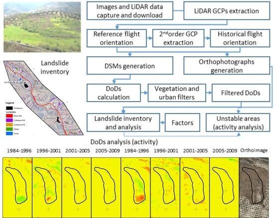
2.3. Methodology
- Orientation of the 2010 reference flight (photogrammetric and LiDAR).
- Orientation of the remaining flights in the same coordinate reference system as the reference flight.
- Generation of the DSMs and orthophotographs.
- Calculation of differential DSMs (DoDs).
- Filtering and masking of DoDs.
- Elaboration of the multitemporal landslide inventory.
2.3.1. Orientation of the Reference Flight
2.3.2. Orientation of the Remaining Flights
2.3.3. Generation of the DSMs and Orthophotographs
2.3.4. Calculation of Differential DSMs (DoDs)
2.3.5. Filtering and Masking of DoDs
2.3.6. Elaboration of the Multitemporal Landslide Inventory
3. Results
3.1. Analysis of the Multitemporal Landslide Inventory
3.2. Analysis of Monitoring Areas
- Area 1 (dominated by collapses and slides; Figure 7) showed some periods with significant rates of general ground descent in 2009–2010 and 2010–2011 (−0.30 and −0.16 m/year, respectively). Sectors with descent rates reached high average rates in the periods 1996–2001, 2009–2010, 2010–2011 and 2011–2013 (0.5–4 m/year), while sectors with ascent rates did so in the period 2011–2013 (1.8 m/year).
- Area 2 (in which slides predominate) presented a general rate of ground descent in the period 2009–2010 (−0.21 m/year). The average descent rates were higher in 1996–2001 and 2009–2010 (0.4–1.6 m/year), with a significant ascent rate only in 1996–2001 (0.33 m/year).
- Area 3 (flows; Figure 8) showed a significant rate of general descent in the periods 2009–2010 and 2011–2013 (−0.11 and −0.07 m/year), with a great descent rate (3.11 m/year) and a moderate ascent rate (1.4 m/year) in 2009–2010.
- Area 4 (flows; Figure 8) showed only a certain general ground descent in the period 2011–2013 (−0.05 m/year), with moderate descent rates in 2009–2010, 2010–2011, 2011–2013 and 2013–2016 (0.5–1.3 m/year) and ascent rates in 2011–2013 and 2013–2016 (0.6–0.7 m/year).
- Area 5 (slides) showed only a significant rate of general descent in the period 2009–2010 (−0.17 m/year), with a moderate descent rate (1.68 m/year) and ascent rate (1.53 m/year) in the same period.
- Area 6 (collapses) presented a rate of ground descent in the periods 2009–2010 and 2010–2011 (−0.14 and −0.05 m/year), with a significant descent rate in 2010–2011 (2.93 m/year) and ascent rate in 2011–2013 (1.48 m/year).
- Area 7 (collapses) showed a remarkable rate of general descent in 2009–2010 (−0.42 m/year), the descent rate being high in the same period (2.57 m/year) without significant ascent rates.
- Area 8 (collapses) also presented a great rate of general descent in the period 2009–2010 (−0.45 m/year), with a significant descent rate in the same period (2.01 m/year).
- Area 9 (collapses in engineering slopes; Figure 9) showed a significant rate of general descent in the periods 1984–1996 and 1996–2001 (−0.13 and −0.26 m/year). Meanwhile, the descent rates were significant in 1984–1996, 1996–2001, 2009–2010 and 2010–2011 (0.6–1.8 m/year), with the ascent rate of 2011–2013 being the only relevant one (0.9 m/year).
- Area 10 (collapses; Figure 9) had a high rate of ground descent in 2009–2010 (−0.59 m/year). It presented significant descent rates in 2009–2010, 2010–2011 and 2011–2013 (1–4 m/year), with a significant ascent rate in 2009–2010 (3.76 m/year).
4. Discussion
4.1. Accuracy and Uncertainties
4.2. Height Differences
4.3. Landslide Inventory and Factor Analysis
4.4. Multitemporal Inventory Analysis
4.5. Analysis of the Monitoring Areas
4.6. Relationships with Rainfall
5. Conclusions
Author Contributions
Funding
Institutional Review Board Statement
Informed Consent Statement
Data Availability Statement
Acknowledgments
Conflicts of Interest
References
- Varnes, D.J. Landslide Hazard Zonation: A Review of Principles and Practice, Natural Hazards; UNESCO: Paris, France, 1984. [Google Scholar]
- Brabb, E.E. The world landslide problem. Episodes 1991, 14, 52–61. [Google Scholar] [CrossRef]
- Guzzetti, F.; Mondini, A.C.; Cardinali, M.; Fiorucci, F.; Santangelo, M.; Chang, K.T. landslide inventory maps: New tools for an old problem. Earth-Sci. Rev. 2012, 112, 42–66. [Google Scholar] [CrossRef] [Green Version]
- Brunsden, D. Mass movements; the research frontier and beyond: A geomorphological approach. Geomorphology 1993, 7, 85–128. [Google Scholar] [CrossRef]
- Chacón, J.; Irigaray, C.; Fernández, T.; El Hamdouni, R. Engineering geology maps: Landslides and geographical information systems (GIS). Bull. Eng. Geol. Environ. 2006, 65, 341–411. [Google Scholar] [CrossRef]
- Metternicht, G.; Hurni, L.; Gogu, R. Remote sensing of landslides: An analysis of the potential contribution to geo-spatial systems for hazard assessment in mountainous environments. Remote Sens. Environ. 2005, 98, 284–303. [Google Scholar] [CrossRef]
- Scaioni, M.; Longoni, L.; Melillo, V.; Papini, M. Remote sensing for landslide investigations: An overview of recent achievements and perspectives. Remote Sens. 2014, 6, 9600–9652. [Google Scholar] [CrossRef] [Green Version]
- Zhao, C.; Lu, Z. Remote sensing of landslides—A review. Remote Sens. 2018, 10, 279. [Google Scholar] [CrossRef] [Green Version]
- Walstra, J.; Chandler, J.H.; Dixon, N.; Dijkstra, T.A. Time for change—Quantifying landslide evolution using historical aerial photographs and modern photogrammetric methods. In The International Archives of the Photogrammetry, Remote Sensing and Spatial Information Sciences, Proceedings of the 20th ISPRS Congress, Istanbul, Turkey, 12–23 July 2004; Altan, O., Ed.; Copernicus Publications: Gottingen, Germany, 2004; Volume 35, Part B4; pp. 475–480. [Google Scholar]
- Cardenal, J.; Delgado, J.; Mata, E.; González-Díez, A.; Remondo, J.; Díaz de Terán, J.R.; Francés, E.; Salas, L.; Bonachea, J.; Olague, I.; et al. The use of digital photogrammetry techniques in landslide instability. In Geodetic Deformation Monitoring: From Geophysical to Geodetic Roles; Gil-Cruz, J., Sanso, F., Eds.; IAG Springer Series: New York, NY, USA, 2006; pp. 259–264. [Google Scholar]
- Prokešová, R.; Kardoš, M.; Medved’ová, A. Landslide dynamics from high-resolution aerial photographs: A case study from the Western Carpathians, Slovakia. Geomorphology 2010, 115, 90–101. [Google Scholar] [CrossRef]
- González-Díez, A.; Fernández-Maroto, G.; Doughty, M.W.; Díaz de Terán, J.R.; Bruschi, V.; Cardenal, J.; Pérez, J.L.; Mata, E.; Delgado, J. Development of a methodological approach for the accurate measurement of slope changes due to landslides, using digital photogrammetry. Landslides 2014, 11, 615–628. [Google Scholar] [CrossRef]
- Sandric, I.; Mihai, B.; Chitu, Z.; Gutu, A.; Savulescu, I. Object-oriented methods for landslides detection using high resolution imagery, morphometric properties and meteorological data. In Proceedings of ISPRS TC VII Symposium—100 Years ISPRS, Vienna, Austria, 5–7 July 2010; Wagner, W., Székely, B., Eds.; ISPRS: Beijing, China, 2010; Volume 38, Part 7B; pp. 486–491. [Google Scholar]
- Dewitte, O.; Jasselette, J.C.; Cornet, Y.; Van Den Eeckhaut, M.; Collignon, A.; Poesen, J.; Demoulin, A. Decadal-scale analysis of ground movements in old landslides in western Belgium. Eng. Geol. 2008, 99, 11–22. [Google Scholar] [CrossRef]
- Corsini, A.; Borgatti, L.; Cervi, F.; Dahne, A.; Ronchetti, F.; Sterzai, P. Estimating mass-wasting processes in active earth slides—Earth flows with time-series of high-resolution DEMs from photogrammetry and airborne LiDAR. Nat. Hazards Earth Syst. Sci. 2009, 9, 433–439. [Google Scholar] [CrossRef]
- Fernández, T.; Pérez, J.L.; Colomo, C.; Cardenal, J.; Delgado, J.; Palenzuela, J.A.; Irigaray, C.; Chacón, J. Assessment of the evolution of a landslide using digital photogrammetry and LiDAR techniques in the Alpujarras Region (Granada, Southeastern Spain). Geosciences 2017, 7, 32. [Google Scholar] [CrossRef] [Green Version]
- Kamps, M.T.; Bouten, W.; Seijmonsbergen, A.C. LiDAR and orthophoto synergy to optimize object-based landscape change: Analysis of an active landslide. Remote Sens. 2017, 9, 805. [Google Scholar] [CrossRef] [Green Version]
- Brückl, E.; Brunner, F.K.; Kraus, K. Kinematics of a deep-seated landslide derived from photogrammetric, GPS and geophysical data. Eng. Geol. 2006, 88, 149–159. [Google Scholar] [CrossRef]
- Eltner, A.; Kaiser, A.; Castillo, C.; Rock, G.; Neugirg, F.; Abellán, A. Image-based surface reconstruction in geomorphometry—Merits, limits and developments. Earth Surf. Dyn. 2016, 4, 359–389. [Google Scholar] [CrossRef] [Green Version]
- Niethammer, U.; James, M.R.; Rothmund, S.; Travelletti, J.; Joswig, M. UAV-based remote sensing of the Super-Sauze landslide: Evaluation and results. Eng. Geol. 2012, 128, 2–11. [Google Scholar] [CrossRef]
- Fernández, T.; Pérez, J.L.; Cardenal, F.J.; Gómez, J.M.; Colomo, C.; Delgado, J. Analysis of landslide evolution affecting olive groves using UAV and photogrammetric techniques. Remote Sens. 2016, 8, 837. [Google Scholar] [CrossRef] [Green Version]
- Rossi, G.; Tanteri, L.; Tofani, V.; Vannocci, P.; Moretti, S.; Casagli, N. Multitemporal UAV surveys for landslide mapping and characterization. Landslides 2018, 15, 1045–1052. [Google Scholar] [CrossRef] [Green Version]
- Peppa, M.V.; Mills, J.P.; Moore, P.; Miller, P.E.; Chambers, J.E. Automated co-registration and calibration in SfM photogrammetry for landslide change detection. Earth Surf. Process. Landf. 2019, 44, 287–303. [Google Scholar] [CrossRef] [Green Version]
- Cardenal, J.; Fernández, T.; Pérez-García, J.L.; Gómez-López, J.M. Measurement of road surface deformation using images captured from UAVs. Remote Sens. 2019, 11, 1507. [Google Scholar] [CrossRef] [Green Version]
- Glenn, N.F.; Streutker, D.R.; Chadwick, D.J.; Thackray, G.D.; Dorsch, S.J. Analysis of LiDAR-derived topographic information for characterizing and differentiating landslide morphology and activity. Geomorphology 2006, 73, 131–148. [Google Scholar] [CrossRef]
- Lin, M.L.; Chen, T.W.; Lin, C.W.; Ho, D.J.; Cheng, K.P.; Yin, H.Y.; Chen, M.C. Detecting large-scale landslides using Lidar data and aerial photos in the Namasha-Liuoguey Area, Taiwan. Remote Sens. 2014, 6, 42–63. [Google Scholar] [CrossRef] [Green Version]
- Tarolli, P. High-resolution topography for understanding Earth surface processes: Opportunities and challenges. Geomorphology 2014, 216, 295–312. [Google Scholar] [CrossRef]
- Li, X.; Cheng, X.; Chen, W.; Chen, G.; Liu, S. Identification of forested landslides using LiDAR data, object-based image analysis, and machine learning algorithms. Remote Sens. 2015, 7, 9705–9726. [Google Scholar] [CrossRef] [Green Version]
- Pradhan, B.; Alsaleh, A. A supervised object-based detection of landslides and man-made slopes using airborne laser scanning Data. In Laser Scanning Applications in Landslide Assessment; Pradhan, B., Ed.; Springer International Publishing: Cham, Switzerland, 2017; pp. 23–50. [Google Scholar]
- Pawluszek-Filipiak, K.; Borkowski, A. On the importance of train-test split ratio of datasets in automatic landslide detection by supervised classification. Remote Sens. 2020, 12, 3054. [Google Scholar] [CrossRef]
- Palenzuela, J.A.; Marsella, M.; Nardinocchi, C.; Pérez, J.L.; Fernández, T.; Chacón, J.; Irigaray, C. Landslide detection and inventory by integrating LiDAR data in a GIS environment. Landslides 2015, 12, 1035–1050. [Google Scholar] [CrossRef]
- Bossi, G.; Cavalli, M.; Crema, S.; Frigerio, S.; Quan Luna, B.; Mantovani, M.; Marcato, G.; Schenato, L.; Pasuto, A. Multi-temporal LiDAR-DTMs as a tool for modelling a complex landslide: A case study in the Rotolon catchment (eastern Italian Alps). Nat. Hazards Earth Syst. Sci. 2015, 15, 715–722. [Google Scholar] [CrossRef] [Green Version]
- Liu, W.; Yamazaki, F.; Maruyama, Y. Detection of earthquake-induced landslides during the 2018 Kumamoto earthquake using multitemporal airborne Lidar data. Remote Sens. 2019, 11, 2292. [Google Scholar] [CrossRef] [Green Version]
- Mora, O.E.; Lenzano, M.G.; Toth, C.K.; Grejner-Brzezinska, D.A.; Fayne, J.V. Landslide change detection based on multi-temporal airborne LiDAR-derived DEMs. Geosciences 2018, 8, 23. [Google Scholar] [CrossRef] [Green Version]
- Fernández, T.; Sánchez-Gómez, M.; García, F.; Pérez-Varela, F. Cartografía de movimientos de ladera en el frente montañoso de la Cordillera Bética en el sector de Jaén. In Geotemas 13, Proceedings of the Actas del VIII Congreso Geológico de España, Oviedo, España, 17–19 June 2012; Fernández, L.P., Fernández, A., Cuesta, A., Bahamonde, J.R., Eds.; Sociedad Geológica de España: Salamanca, Spain, 2012; Volume 13, pp. 1471–1474. (In Spanish) [Google Scholar]
- Fernández, T.; Pérez, J.L.; Cardenal, F.J.; López, A.; Gómez, J.M.; Colomo, C.; Sánchez, M.; Delgado, J. Use of a light UAV and photogrammetric techniques to study the evolution of a landslide in Jaén (Southern Spain). Int. Arch. Photogramm. Remote Sens. Spat. Inf. Sci. 2015, 40, 241. [Google Scholar] [CrossRef] [Green Version]
- Carpena, R.L.; Mellado, I.; Moya, F.; Colomo, C.; Bédmar, P.; Calero, J.; Pérez, A.; Fernández, T.; Sánchez-Gómez, M.; Tovas, J. Análisis de riesgos asociados a las infraestructuras viarias de la Diputación Provincial de Jaén. In Proceedings of the IX Simposio Nacional Sobre Laderas y Taludes Inestables, Santander, Spain, 27–30 June 2017; Volume 1, pp. 335–346. (In Spanish). [Google Scholar]
- Varnes, D.J. Slope movement, types and processes. In Landslides: Analysis and Control; Schuster, R.L., Krizek, R.J., Eds.; Transportation Research Board Special Report National Academy of Sciences: Washington, DC, USA, 1978; Volume 176, pp. 12–33. [Google Scholar]
- Hungr, O.; Leroueil, S.; Picarelli, L. The Varnes classification of landslide types, an update. Landslides 2014, 11, 167–194. [Google Scholar] [CrossRef]
- Roldán, F.J.; Lupiani, E.; Jerez, L. Mapa Geológico de España, Escala 1:50.000, Mapa y Memoria Explicativa; Instituto Geológico Nacional: Madrid, Spain, 1988. (In Spanish) [Google Scholar]
- Pérez-Valera, F.; Sánchez-Gómez, M.; Pérez-López, A.; Pérez-Valera, L.A. An evaporite-bearing accretionary complex in the northern front of the Betic-Rif orogeny. Tectonics 2017, 36, 1006–1036. [Google Scholar] [CrossRef] [Green Version]
- Instituto Geográfico Nacional (IGN), Fototeca Digital. Available online: http://fototeca.cnig.es/ (accessed on 31 January 2021).
- Instituto de Estadística y Cartografía de Andalucía (IECA), Fototeca. Available online: http://www.juntadeandalucia.es/institutodeestadisticaycartografia/fototeca/ (accessed on 31 January 2021).
- Colomo-Jiménez, C.; Pérez-García, J.L.; Fernández-del-Castillo, T.; Gómez-López, J.M.; Mozas-Calvache, A.M. Methodology for orientation and fusion of photogrammetric and LiDAR data for multitemporal studies. Int. Arch. Photogramm. Remote Sens. Spat. Inf. Sci. 2016, XLI-B7, 639–645. [Google Scholar] [CrossRef]
- Fernández, T.; Pérez-García, J.L.; Gómez-López, J.M.; Cardenal, J.; Calero, J.; Sánchez-Gómez, M.; Delgado, J.; Tovar-Pescador, J. Multitemporal analysis of Gully erosion in olive groves by means of digital elevation models obtained with aerial photogrammetric and LiDAR data. ISPRS Int. J. Geo-Inf. 2020, 9, 260. [Google Scholar] [CrossRef] [Green Version]
- Socet Set 5.6; Bae Systems Plc.: London, UK, 2011.
- Korsgaard, N.; Nuth, C.; Khan, S.; Kjeldsen, K.K.; Bjørk, A.A.; Schomacker, A.; Kjaer, K.H. Digital elevation model and orthophotographs of Greenland based on aerial photographs from 1978–1987. Sci. Data 2016, 3, 160032. [Google Scholar] [CrossRef] [PubMed] [Green Version]
- QGIS 3. A Free and Open Source Geographic Information System. 2020. Available online: https://www.qgis.org/en/site/ (accessed on 31 January 2021).
- Brasington, J.; Rumsby, B.T.; McVey, R.A. Monitoring and modelling morphological change in a braided gravel-bedriver using high resolution GPS-based survey. Earth Surf. Proc. Landf. 2000, 25, 973–990. [Google Scholar] [CrossRef]
- Instituto de Estadística y Cartografía de Andalucía (IECA), Localizador de Información Geográfica de Andalucía. Available online: http://www.juntadeandalucia.es/institutodeestadisticaycartografia/lineav2/web/ (accessed on 31 January 2021).
- Bannari, A.; Morin, D.; Bonn, F.; Huete, A.R. A review of vegetation indices. Remote Sens. Rev. 1995, 13, 95–120. [Google Scholar] [CrossRef]
- Louhaichi, M.; Borman, M.M.; Johnson, D.E. Spatially located platform and aerial photography for documentation of grazing impacts on wheat. Geocarto Int. 2001, 16, 65–70. [Google Scholar] [CrossRef]
- Wheaton, J.M.; Brasington, J.; Darby, S.E.; Sear, D.A. Accounting for uncertainty in DEMs from repeat topographic surveys: Improved sediment budgets. Earth Surf. Process. Landf. 2010, 35, 136–156. [Google Scholar] [CrossRef]
- Hattanji, T.; Moriwaki, H. Morphometric analysis of relic landslides using detailed landslide distribution maps: Implications for forecasting travel distance of future landslides. Geomorphology 2009, 103, 447–454. [Google Scholar] [CrossRef] [Green Version]
- International Union of Geological Sciences Working Group on Landslides. A suggested method for describing the rate of movement of a landslide. Bull. Eng. Geol. Environ. 1995, 52, 75–78. [Google Scholar]
- WP/WLI. A suggested method for describing the activity of a landslide. Bull. Eng. Geol. Environ. 1993, 47, 53–57. [Google Scholar]
- Boussouf, S.; Irigaray, C.; Chacón, J. Movimientos de ladera y factores determinantes en la vertiente septentrional de la Depresión de Granada (sector Colomera-Zagra). Rev. Soc. Geol. España 1994, 7, 251–260. (In Spanish) [Google Scholar]
- Irigaray, C.; Fernández, T.; El Hamdouni, R.; Chacón, J. Verification of landslide susceptibility mapping. A case study. Earth Surf. Proc. Land. 1999, 24, 537–554. [Google Scholar]
- Irigaray, C.; Fernández, T.; El Hamdouni, R.; Chacón, J. Evaluation and validation of landslide susceptibility maps obtained by a GIS matrix method: Examples from the Betic Cordillera (southern Spain). Nat. Hazards 2007, 41, 61–79. [Google Scholar] [CrossRef]
- Reichenbach, P.; Rossi, M.; Malamud, B.; Mihri, M.; Guzzetti, F. A review of statistically-based landslide susceptibility models. Earth-Sci. Rev. 2018, 180, 60–91. [Google Scholar] [CrossRef]
- IAEG. Commission on Landslides. Suggested nomenclature for landslides. Bull. Eng. Geol. Environ. 1990, 41, 13–16. [Google Scholar]
- Guzzetti, F.; Reichenbach, P.; Cardinali, M.; Galli, M.; Ardizzone, F. Probabilistic landslide hazard assessment at the basin scale. Geomorphology 2005, 72, 272–299. [Google Scholar] [CrossRef]
- Crozier, M.J. Techniques for the morphometric analysis of landslips. Z. Geomorphol. 1973, 17, 78–101. [Google Scholar]
- Finlay, P.J.; Fell, R.; Maguire, P.K. The relationship between the probability of landslide occurrence and rainfall. Can. Geotech. J. 1997, 34, 811–824. [Google Scholar] [CrossRef]
- Guzzeti, F. Landslide hazard assessment and risk evaluation: Limits and prospectives. In Proceedings of the 4th EGS Plinius Conference, Mediterranean Storms, Mallorca, Spain, 2–4 October 2002. [Google Scholar]
- Trigo, R.M.; Pozo, D.; Timothy, C.; Osborn, J.; Castro, Y.; Gámiz, S.; Esteban, M.J. NAO influence on precipitation, river flow and water resources in the Iberian Peninsula. Int. J. Clim. 2004, 24, 925–944. [Google Scholar] [CrossRef]


| Aerial Image Properties | ||||||
|---|---|---|---|---|---|---|
| Date | Bands | Format | Scale | Camera | Digitalization Resolution (mm) | GSD (m) |
| 1984 | Panchromatic | Film | 1:30,000 | Wild RC10 | 0.025 | 0.75 |
| 1996 | Panchromatic | Film | 1:20,000 | Wild RC10 | 0.020 | 0.30 |
| 2001 | Panchromatic | Film | 1:20,000 | Leica RC30 | 0.015 | 0.30 |
| 2005 | CIR | Film | 1:30,000 | Leica RC30 | 0.015 | 0.45 |
| 2009 | RGB | Digital | 1:30,000 | Z/I DMC120 | --- | 0.45 |
| 2010 1 | RGB–NIR | Digital | 1:10,000 | Z/I DMC | --- | 0.20 |
| 2011 | RGB | Digital | 1:30,000 | Z/I DMC120 | --- | 0.45 |
| 2013 | RGB | Digital | 1:30,000 | Vexcel UCXp | --- | 0.45 |
| 2016 | RGB–NIR | Digital | 1:30,000 | Vexcel UCXp | --- | 0.45 |
| LiDAR dataset | ||||||
| Date | System | Points /m2 | ||||
| 2010 | Leica ALS50-II | 1–1.5 | ||||
| Date | Number of Photographs | GCP-Type 2 Number | Tie Points Number | RMS (Pixel) | RMS GCP Error (m) | RMS Prop. Error (m) | ||
|---|---|---|---|---|---|---|---|---|
| RMSXY | RMSZ | RMSXY | RMSZ | |||||
| 1984 | 30 | 28xyz, 26z | 162 | 0.507 | 0.266 | 0.084 | 0.268 | 0.125 |
| 1996 | 38 | 20 xyz | 178 | 0.474 | 0.172 | 0.136 | 0.175 | 0.165 |
| 2001 | 32 | 9xyz | 140 | 0.571 | 0.067 | 0.093 | 0.073 | 0.132 |
| 2005 | 32 | 11xyz,19z | 164 | 0.637 | 0.049 | 0.133 | 0.057 | 0.162 |
| 2009 | 33 | 15xyz,9z | 186 | 0.506 | 0.027 | 0.200 | 0.040 | 0.221 |
| 2010 1 | 98 | 25 z | 649 | 0.328 | 0.030 | 0.093 | - | - |
| 2011 | 35 | 33xyz,17z | 201 | 0.376 | 0.139 | 0.110 | 0.142 | 0.144 |
| 2013 | 31 | 27xyz | 211 | 0.570 | 0.068 | 0.044 | 0.074 | 0.103 |
| 2016 | 22 | 16xyz | 122 | 0.604 | 0.052 | 0.035 | 0.060 | 0.099 |
| Date | Z Propag. Error (m) | Uncert. in DSMs (m) | Period | Uncert. in DoDs (m) |
|---|---|---|---|---|
| 1984 | 0.125 | 0.313 | ||
| 1996 | 0.165 | 0.413 | 1984–1996 | 0.518 |
| 2001 | 0.132 | 0.330 | 1996–2001 | 0.528 |
| 2005 | 0.162 | 0.405 | 2001–2005 | 0.522 |
| 2009 | 0.221 | 0.553 | 2005–2009 | 0.685 |
| 2010 | 0.093 | 0.233 | 2009–2010 | 0.599 |
| 2011 | 0.144 | 0.360 | 2010–2011 | 0.429 |
| 2013 | 0.103 | 0.258 | 2011–2013 | 0.443 |
| 2016 | 0.099 | 0.248 | 2013–2016 | 0.357 |
| Date | Typol. | Nº | %N | Tot.Area 1 | %TA | Area 1 | Perim. 2 | H. Int. 2 | H/L | Height 2 | Slope 3 | Orien. 3 | DoD 2 | Lithol. |
|---|---|---|---|---|---|---|---|---|---|---|---|---|---|---|
| 1984 – 1996 | R. Falls | 0 | 0.00 | - | - | - | - | - | - | - | - | - | - | - |
| Col-NS | 66 | 80.49 | 107,819 | 69.22 | 1634 | 169 | 21.22 | 0.47 | 609 | 29.27 | 150 | −0.61 | 6 | |
| Slides | 10 | 12.20 | 24,163 | 15.51 | 2416 | 179 | 26.80 | 0.48 | 528 | 23.31 | 355 | −0.54 | 2 | |
| Flows | 3 | 3.66 | 20,097 | 12.90 | 6699 | 308 | 33.00 | 0.18 | 543 | 25.70 | 328 | 0.16 | 2 | |
| Col-ES | 3 | 3.66 | 3678 | 2.36 | 1226 | 191 | 13.95 | 0.53 | 735 | 31.94 | 140 | −2.00 | 2 | |
| Total | 82 | 100 | 155,757 | 100 | 1899 | 176 | 22.07 | 0.43 | 602 | 28.51 | 142 | −0.53 | 6 | |
| 1996 – 2001 | R. Falls | 0 | 0.00 | - | - | - | - | - | - | - | - | - | - | - |
| Col-NS | 72 | 54.55 | 55.631 | 31.92 | 773 | 126 | 16.19 | 0.52 | 615 | 33.13 | 91 | -1.33 | 6 | |
| Slides | 17 | 12.88 | 70,745 | 40.59 | 4065 | 242 | 26.83 | 0.37 | 569 | 23.00 | 101 | -0.96 | 2 | |
| Flows | 5 | 3.79 | 20,850 | 11.96 | 4170 | 269 | 25.36 | 0.17 | 560 | 17.33 | 356 | -0.17 | 2 | |
| Col-ES | 38 | 28.79 | 27,049 | 15.52 | 665 | 131 | 11.05 | 0.57 | 620 | 28.86 | 61 | -1.79 | 8 | |
| Total | 132 | 100 | 174,275 | 100 | 1320 | 149 | 16.81 | 0.43 | 605 | 28.87 | 82 | -1.11 | 8 | |
| 2001 – 2005 | R. Falls | 0 | 0.00 | - | - | - | - | - | - | - | - | - | - | - |
| Col-NS | 16 | 50.00 | 13,517 | 19.70 | 845 | 173 | 17.03 | 0.52 | 619 | 36.71 | 216 | −1.35 | 8 | |
| Slides | 4 | 12.50 | 33,588 | 48.96 | 8397 | 403 | 48.26 | 0.47 | 677 | 31.24 | 77 | −0.13 | 3 | |
| Flows | 1 | 3.13 | 7837 | 11.42 | 7837 | 365 | 28.29 | 0.14 | 509 | 15.01 | 68 | −0.13 | 2 | |
| Col-ES | 11 | 34.38 | 13,663 | 19.92 | 1242 | 183 | 15.62 | 0.59 | 644 | 30.28 | 4 | −1.77 | 2 | |
| Total | 32 | 100 | 68,605 | 100 | 2144 | 211 | 20.80 | 0.46 | 632 | 33.14 | 68 | −0.70 | 8 | |
| 2005 – 2009 | R. Falls | 0 | 0.00 | - | - | - | - | - | - | - | - | - | - | - |
| Col-NS | 25 | 75.76 | 15,262 | 78.98 | 610 | 110 | 15.57 | 0.56 | 619 | 30.42 | 334 | −1.11 | 6 | |
| Slides | 1 | 3.03 | 1398 | 7.23 | 1398 | 178 | 11.72 | 0.28 | 571 | 25.03 | 238 | −0.46 | 8 | |
| Flows | 0 | 0.00 | - | - | - | - | - | - | - | - | - | - | - | |
| Col-ES | 7 | 21.21 | 2664 | 13.79 | 381 | 115 | 9.40 | 0.64 | 598 | 26.48 | 34 | −1.20 | 2 | |
| Total | 33 | 100 | 19,324 | 100 | 586 | 113 | 14.15 | 0.55 | 613 | 29.42 | 337 | −1.08 | 6 | |
| 2009 – 2010 | R. Falls | 1 | 0.51 | 268 | 0.08 | 268 | 70 | 43.29 | 2.23 | 990 | 59.88 | 187 | −3.29 | 1 |
| Col-NS | 118 | 60.20 | 129,192 | 36.75 | 1095 | 158 | 18.65 | 0.50 | 628 | 29.75 | 315 | −1.38 | 6 | |
| Slides | 26 | 13.27 | 113,848 | 32.39 | 4379 | 260 | 35.35 | 0.47 | 582 | 27.13 | 205 | −1.18 | 2 | |
| Flows | 6 | 3.06 | 54,691 | 15.56 | 9115 | 361 | 39.27 | 0.18 | 583 | 21.44 | 53 | −0.25 | 2 | |
| Col-ES | 45 | 22.96 | 53,525 | 15.23 | 1189 | 191 | 15.23 | 0.59 | 627 | 29.84 | 194 | −1.50 | 6 | |
| Total | 196 | 100 | 351,524 | 100 | 1801 | 185 | 20.84 | 0.46 | 621 | 29.16 | 254 | −1.16 | 6 | |
| 2010 – 2011 | R. Falls | 0 | 0.00 | - | - | - | - | - | - | - | - | - | - | - |
| Col-NS | 85 | 61.59 | 72,920 | 33.53 | 858 | 133 | 16.68 | 0.50 | 616 | 29.52 | 186 | −1.10 | 6 | |
| Slides | 19 | 13.77 | 73,320 | 33.71 | 3859 | 225 | 27.23 | 0.39 | 586 | 23.42 | 195 | −1.37 | 6 | |
| Flows | 2 | 1.45 | 35,100 | 16.14 | 17,550 | 495 | 53.71 | 0.18 | 630 | 20.51 | 50 | 0.00 | 2 | |
| Col-ES | 32 | 23.19 | 36,135 | 16.62 | 1129 | 177 | 12.96 | 0.51 | 629 | 28.04 | 248 | −1.37 | 6 | |
| Total | 138 | 100 | 217,475 | 100 | 1576 | 161 | 17.81 | 0.41 | 615 | 28.21 | 194 | −1.06 | 6 | |
| 2011 – 2013 | R. Falls | 0 | 0.00 | - | - | - | - | - | - | - | - | - | - | - |
| Col-NS | 94 | 63.09 | 124,785 | 37.94 | 1327 | 160 | 20.26 | 0.49 | 594 | 28.75 | 331 | −1.33 | 6 | |
| Slides | 22 | 14.77 | 106,383 | 32.35 | 4836 | 276 | 35.77 | 0.46 | 563 | 26.12 | 89 | −0.92 | 2 | |
| Flows | 4 | 2.68 | 58,341 | 17.74 | 14,585 | 484 | 39.41 | 0.14 | 585 | 15.86 | 55 | −0.33 | 2 | |
| Col-ES | 29 | 19.46 | 39,373 | 11.97 | 1358 | 178 | 17.54 | 0.63 | 592 | 28.61 | 53 | −1.79 | 8 | |
| Total | 149 | 100 | 328,882 | 100.00 | 2207 | 190 | 22.54 | 0.44 | 589 | 27.99 | 37 | −1.08 | 6 | |
| 2013 – 2016 | R. Falls | 0 | 0.00 | - | - | - | - | - | - | - | - | - | - | - |
| Col-NS | 52 | 70.27 | 43,096 | 30.05 | 829 | 134 | 18.12 | 0.56 | 637 | 32.19 | 184 | −1.48 | 6 | |
| Slides | 4 | 5.41 | 36,132 | 25.20 | 9033 | 372 | 58.69 | 0.55 | 685 | 30.86 | 207 | −0.33 | 3 | |
| Flows | 2 | 2.70 | 51,389 | 35.84 | 25,695 | 852 | 66.38 | 0.18 | 609 | 12.68 | 54 | 0.06 | 2 | |
| Col-ES | 16 | 21.62 | 12,777 | 8.91 | 799 | 153 | 14.05 | 0.66 | 610 | 32.68 | 251 | −2.25 | 8 | |
| Total | 74 | 100 | 143,395 | 100.00 | 1938 | 170 | 20.74 | 0.43 | 633 | 31.69 | 168 | −0.71 | 6 | |
| 1984 – 2016 | R. Falls | 1 | 0.12 | 266 | 0.03 | 268 | 70 | 43.29 | 2.23 | 990 | 59.88 | 187 | −3.29 | 1 |
| Col-NS | 528 | 63.16 | 455,609 | 46.63 | 1065 | 147 | 18.84 | 0.51 | 614 | 30.11 | 264 | −1.18 | 6 | |
| Slides | 103 | 12.32 | 244,193 | 24.99 | 4446 | 255 | 35.13 | 0.47 | 589 | 26.06 | 147 | −0.94 | 2 | |
| Flows | 23 | 2.75 | 115,147 | 11.78 | 10,796 | 410 | 44.93 | 0.19 | 588 | 17.98 | 44 | −0.13 | 2 | |
| Col-ES | 181 | 21.65 | 161,943 | 16.57 | 1034 | 167 | 14.55 | 0.60 | 621 | 29.32 | 176 | −1.65 | 8 | |
| Total | 836 | 100 | 977,157 | 100.00 | 1747 | 172 | 20.32 | 0.48 | 610 | 29.09 | 104 | 0.00 | 6 |
| Area | Typology | H. Aver. | H. Min. | H. Max. | H. Range | Slope | Ori. | Lithol. |
|---|---|---|---|---|---|---|---|---|
| 1 | Col-NS | 485 | 464 | 509 | 44.65 | 35.90 | 347 | 2 |
| 2 | Slides | 498 | 482 | 513 | 31.11 | 26.66 | 21 | 2 |
| 3 | Flows | 580 | 557 | 605 | 47.51 | 13.16 | 346 | 2 |
| 4 | Flows | 629 | 577 | 671 | 94.04 | 11.06 | 38 | 8 |
| 5 | Slides | 569 | 543 | 598 | 55.20 | 23.57 | 282 | 2 |
| 6 | Col-NS | 576 | 557 | 596 | 39.80 | 30.62 | 192 | 6 |
| 7 | Col-NS | 643 | 629 | 657 | 27.66 | 36.90 | 153 | 6 |
| 8 | Col-NS | 773 | 757 | 792 | 34.78 | 30.07 | 279 | 2 |
| 9 | Col-ES | 662 | 641 | 688 | 47.87 | 34.02 | 250 | 3 |
| 10 | Col-NS | 727 | 703 | 752 | 48.65 | 36.39 | 200 | 3 |
| All | Col-NS | 620 | 599 | 642 | 42.61 | 31.01 | 185 | 2 |
| Rates of height differences (DoD) | ||||||||
| Area | 1984–1996 | 1996–2001 | 2001–2005 | 2005–2009 | 2009–2010 | 2010–2011 | 2011–2013 | 2013–2016 |
| 1 | 0.00 | −0.01 | 0.01 | 0.01 | −0.30 | −0.16 | −0.03 | 0.01 |
| 2 | 0.00 | −0.01 | 0.01 | 0.01 | −0.21 | 0.03 | −0.05 | 0.00 |
| 3 | 0.00 | 0.00 | 0.00 | 0.01 | −0.11 | −0.04 | −0.07 | 0.01 |
| 4 | 0.00 | −0.01 | 0.00 | 0.00 | −0.03 | 0.00 | −0.05 | 0.01 |
| 5 | 0.00 | −0.01 | −0.01 | 0.02 | −0.17 | −0.04 | −0.03 | 0.00 |
| 6 | −0.01 | −0.02 | 0.01 | 0.02 | −0.14 | −0.05 | −0.03 | −0.01 |
| 7 | 0.00 | 0.00 | −0.02 | 0.03 | −0.42 | −0.03 | −0.02 | 0.01 |
| 8 | 0.00 | 0.00 | 0.00 | 0.01 | −0.45 | 0.04 | −0.03 | −0.02 |
| 9 | −0.13 | −0.26 | 0.01 | 0.02 | −0.10 | −0.09 | −0.01 | 0.00 |
| 10 | 0.02 | −0.09 | 0.02 | 0.01 | −0.59 | −0.16 | −0.02 | −0.02 |
| All | −0.01 | −0.05 | 0.00 | 0.01 | −0.24 | −0.05 | −0.03 | 0.00 |
| Rates of height differences in sector with descents | ||||||||
| Area | 1984–1996 | 1996–2001 | 2001–2005 | 2005–2009 | 2009–2010 | 2010–2011 | 2011–2013 | 2013–2016 |
| 1 | −0.14 | −0.53 | −0.43 | −0.41 | −2.05 | −3.99 | −1.36 | −0.66 |
| 2 | −0.12 | −0.40 | −0.43 | −0.53 | −1.61 | −1.44 | −1.01 | −0.73 |
| 3 | −0.10 | −0.37 | −0.37 | −0.28 | −3.11 | −1.10 | −0.58 | −0.57 |
| 4 | −0.16 | −0.28 | −0.33 | −0.37 | −1.28 | −1.34 | −0.69 | −0.51 |
| 5 | −0.11 | −0.27 | −0.36 | −0.39 | −1.68 | −1.38 | −0.65 | −0.50 |
| 6 | −0.42 | −0.27 | −0.40 | −0.38 | −1.31 | −2.93 | −1.22 | −0.71 |
| 7 | −0.11 | −0.31 | −0.45 | −0.55 | −2.57 | −1.59 | −0.81 | −0.81 |
| 8 | −0.20 | −0.30 | −0.42 | −0.39 | −2.01 | −1.40 | −0.90 | −0.60 |
| 9 | −0.57 | −0.82 | −0.56 | −0.39 | −1.76 | −1.38 | −0.82 | −0.60 |
| 10 | −0.23 | −0.50 | −0.88 | −0.63 | −4.10 | −1.75 | −0.85 | −0.78 |
| All | −0.32 | −0.52 | −0.50 | −0.46 | −2.65 | −2.60 | −0.99 | −0.66 |
| Rates of height differences in sector with ascents | ||||||||
| Area | 1984–1996 | 1996–2001 | 2001–2005 | 2005–2009 | 2009–2010 | 2010–2011 | 2011–2013 | 2013–2016 |
| 1 | 0.17 | 0.32 | 0.45 | 0.44 | 1.69 | 2.47 | 1.80 | 0.60 |
| 2 | 0.12 | 0.33 | 0.48 | 0.43 | 1.88 | 1.61 | 0.78 | 0.59 |
| 3 | 0.27 | 0.28 | 0.36 | 0.47 | 1.41 | 1.10 | 0.00 | 0.46 |
| 4 | 0.12 | 0.46 | 0.36 | 0.61 | 1.58 | 1.52 | 0.71 | 0.57 |
| 5 | 0.10 | 0.27 | 0.36 | 0.40 | 1.53 | 1.27 | 0.65 | 0.49 |
| 6 | 0.14 | 0.34 | 0.36 | 0.34 | 1.51 | 2.14 | 1.48 | 0.56 |
| 7 | 0.13 | 0.33 | 0.37 | 0.68 | 2.15 | 1.48 | 1.16 | 0.54 |
| 8 | 0.13 | 0.29 | 0.40 | 0.54 | 1.41 | 1.52 | 0.88 | 0.56 |
| 9 | 0.22 | 0.47 | 0.45 | 0.47 | 1.45 | 1.35 | 0.86 | 0.51 |
| 10 | 0.49 | 0.38 | 0.68 | 0.82 | 3.76 | 2.42 | 1.25 | 0.66 |
| All | 0.26 | 0.36 | 0.50 | 0.61 | 2.35 | 1.98 | 1.29 | 0.58 |
Publisher’s Note: MDPI stays neutral with regard to jurisdictional claims in published maps and institutional affiliations. |
© 2021 by the authors. Licensee MDPI, Basel, Switzerland. This article is an open access article distributed under the terms and conditions of the Creative Commons Attribution (CC BY) license (https://creativecommons.org/licenses/by/4.0/).
Share and Cite
Fernández, T.; Pérez-García, J.L.; Gómez-López, J.M.; Cardenal, J.; Moya, F.; Delgado, J. Multitemporal Landslide Inventory and Activity Analysis by Means of Aerial Photogrammetry and LiDAR Techniques in an Area of Southern Spain. Remote Sens. 2021, 13, 2110. https://doi.org/10.3390/rs13112110
Fernández T, Pérez-García JL, Gómez-López JM, Cardenal J, Moya F, Delgado J. Multitemporal Landslide Inventory and Activity Analysis by Means of Aerial Photogrammetry and LiDAR Techniques in an Area of Southern Spain. Remote Sensing. 2021; 13(11):2110. https://doi.org/10.3390/rs13112110
Chicago/Turabian StyleFernández, Tomás, José L. Pérez-García, José M. Gómez-López, Javier Cardenal, Francisco Moya, and Jorge Delgado. 2021. "Multitemporal Landslide Inventory and Activity Analysis by Means of Aerial Photogrammetry and LiDAR Techniques in an Area of Southern Spain" Remote Sensing 13, no. 11: 2110. https://doi.org/10.3390/rs13112110