Article

A Downscaling–Merging Scheme for Improving Daily Spatial Precipitation Estimates Based on Random Forest and Cokriging

1
State Key Laboratory of Water Resources and Hydropower Engineering Science, Wuhan University, Wuhan 430072, China
2
Information Center (Hydrology Monitor and Forecast Center), Ministry of Water Resources of the People’s Republic of China, Beijing 100053, China
*
Author to whom correspondence should be addressed.
Remote Sens. 2021, 13(11), 2040; https://doi.org/10.3390/rs13112040
Submission received: 8 April 2021 / Revised: 19 May 2021 / Accepted: 19 May 2021 / Published: 21 May 2021
(This article belongs to the Special Issue Measurement of Hydrologic Variables with Remote Sensing)

Abstract

:
High-spatial-resolution precipitation data are of great significance in many applications, such as ecology, hydrology, and meteorology. Acquiring high-precision and high-resolution precipitation data in a large area is still a great challenge. In this study, a downscaling–merging scheme based on random forest and cokriging is presented to solve this problem. First, the enhanced decision tree model, which is based on random forest from machine learning algorithms, is used to reduce the spatial resolution of satellite daily precipitation data to 0.01°. The downscaled satellite-based daily precipitation is then merged with gauge observations using the cokriging method. The scheme is applied to downscale the Global Precipitation Measurement Mission (GPM) daily precipitation product over the upstream part of the Hanjiang Basin. The experimental results indicate that (1) the downscaling model based on random forest can correctly spatially downscale the GPM daily precipitation data, which retains the accuracy of the original GPM data and greatly improves their spatial details; (2) the GPM precipitation data can be downscaled on the seasonal scale; and (3) the merging method based on cokriging greatly improves the accuracy of the downscaled GPM daily precipitation data. This study provides an efficient scheme for generating high-resolution and high-quality daily precipitation data in a large area.

Graphical Abstract

1. Introduction

As an important part of the energy and material cycles, precipitation is of great significance to hydrology, meteorology, and ecology [1,2,3]. The surface process is mostly affected by precipitation, an essential input parameter of surface meteorology in various plant physiology models, ecology, hydrology, and other fields [4,5,6,7]. Most of the uncertainties in land hydrological processes are caused by the spatiotemporal variability of precipitation [8,9]. Therefore, acquiring high-resolution and high-precision precipitation data is essential for researching surface processes and global climate change.
At present, precipitation is mainly measured by the rain gauge, satellite remote sensing, and weather radar. Traditional rain gauges can provide relatively accurate rainfall values on the point scales, but they are not accurate for estimating continuous spatial precipitation distributions on a large scale [10]. Meteorological radar can provide more precise rainfall data with spatial and temporal resolution. However, weather radar has many disadvantages, such as measurement error caused by beam obscuration and distance attenuation in complex terrain [11]. Since the 1980s, satellite precipitation observation based on remote sensing technology has developed rapidly, such as the Geostationary Operational Environmental Satellite (GOES), the MeteoSat, the National Oceanic and Atmospheric Administration–Polar Orbiting Environmental Satellites (NOAA–POES), the Tropical Precipitation Measurement Mission (TRMM) [12], Global Precipitation Satellite Mapping (GSMaP) [13], the Global Precipitation Climate Plan (GPCP) [14], and the Global Precipitation Measurement Mission (GPM) [15]. The satellite precipitation observation data provide reliable precipitation estimates and reflect more spatial distributions than the rain gauge data. For satellite precipitation observation, it is impossible to achieve high temporal resolution and high spatial resolution simultaneously (such as 0.25° from the TRMM and 0.1° from the GPM). The spatial resolution of the satellite precipitation data is too low for local basin hydrological research. The spatial downscaling is an effective way to solve this problem to expand the application range of satellite precipitation data [16].
There are usually two methods for the spatial downscaling of precipitation: dynamic and statistical downscaling. Dynamic downscaling relies on regional climate or numerical weather models and provides high-resolution precipitation by simulating physical processes of the land–atmosphere coupling system, usually requiring considerable computational resources [17]. Statistical downscaling is a downscaling model constructed by the significant relationship between environmental variables and precipitation, and high-resolution precipitation is then inferred using high-resolution environmental variables. Statistical downscaling has been widely applied to spatial downscaling of satellite precipitation data. The normalized vegetation index (NDVI) was independently used as the explanatory variable to downscale the annual TRMM data for the first time in the Iberian Peninsula [18]. Jia et al. [19] improved the accuracy of the downscaled annual TRMM data using DEM and NDVI as explanatory variables. Fang et al. [20] indicated that the effects of topography factors such as aspect, slope, and terrain roughness on the spatial downscale of TRMM data should be considered. After that, environmental variables such as topography (elevation, slope, aspect), vegetation (NDVI), land surface temperature (LST), and geographical location (longitude and latitude) were widely used in the spatial downscaling of TRMM, GPM, and other data at an annual or monthly scale [21,22,23,24]. The correlation between environmental variables and precipitation at a daily scale is not clear, so Ma [25] and Chen [26] et al. tried to downscale the satellite annual precipitation data accumulated by daily precipitation using the regression model and then disassembled the downscaled annual precipitation data into a daily scale to obtain downscaled satellite daily precipitation data.
Since there is no additional precise precipitation observation in the downscaling process, the original satellite precipitation data affect the accuracy of downscaling results. Many studies have found that the time scale certainly influences the accuracy of satellite precipitation data. The accuracy of low time resolution (monthly or yearly) satellite precipitation data is higher than that of high time resolution (day or finer time scale) satellite precipitation data [27,28]. Therefore, it is certain that the accuracy of high temporal resolution downscaled satellite precipitation data is also inferior. In recent years, to reduce errors in satellite precipitation estimation and improve its accuracy, the method of merging satellite-based precipitation data with gauge observation data has become a common approach, such as statistical bias correction [29], inverse root mean square error (IRMSE) weighting [30], random forest [31], geographic differential analysis (GDA) [32], kriging with external drift (KED) [33], and cokriging (CK).
A downscaling–merging (DM) scheme based on random forest and cokriging was adopted in this study. By merging the downscaled satellite precipitation with the gauge observations, daily precipitation data with high accuracy were obtained. By taking the upstream of the Hanjiang River Basin (above the Danjiangkou Reservoir) as a case study, the effectiveness of the method was verified by GPM daily precipitation data.

2. Study Area and Data

2.1. Study Area

The study region is the upstream part of the Hanjiang Basin, which is the largest tributary in the Yangtze River and the water source of the Middle Route Project of South to North Water Transfer, China (Figure 1). It originates from Qinling Mountain and is located in the southeast of China between east longitude of 106°15′–112°00′ and north latitude of 30°10′–34°20′. The entire drainage area of the study region is about 960,000 km2. The basin has a subtropical monsoon climate with humid air and plentiful rainfall. The annual average rainfall is roughly 830 mm, decreasing from south to north.

2.2. Datasets

The Global Precipitation Measurement (GPM) is an international satellite mission launched by the National Aeronautics and Space Administration and the Japan Aerospace Exploration Agency on 28 February 2014. IMERG (Integrated Multi-satellite Retrievals for GPM) is the level 3 multi-satellite precipitation algorithm of GPM, which combines precipitation information measured from the microwave sensor and infrared sensors onboard GPM constellations and [34] monthly gauge precipitation data. IMERG calculates precipitation estimates partly from passive microwave (PMW) sensors on the GPM satellite platform using the 2014 version of the Goddard Section Algorithm (GPROF2014), which is a significant improvement over TMPA (GPROF2010) [35,36]. The GPM IMERG data as of March 2014 is available and can be downloaded from http://pmm.nasa.gov/data-access/downloads/gpm/, (accessed on 28 September 2020) This study used the GPM IMERG Final Precipitation L3 1 day 0.1° × 0.1° V06 (GPM_3IMERGDF) as the daily satellite precipitation products.
The monthly NDVI (MOD13A3) data of the study area were acquired from the NASA Land Processes Distributed Active Archive Center (LP DAAC) from https://lpdaac.usgs.gov/products/mod13a3v006/, (accessed on 13 October 2020) which have a 1 km spatial resolution. Land surface temperature (LST) data were derived from MODIS (Moderate-resolution Imaging Spectroradiometer) sensors on Terra and Aqua satellites, which provide day and night global surface temperature records with errors between –1K and 1K. MOD11A2 products have a 1 km spatial resolution and an eight-day time resolution and can be downloaded from https://lpdaac.usgs.gov/products/mod11a2v006/, (accessed on 20 October 2020). The DEM (Digital Elevation Model) data were downloaded from the NASA Shuttle Radar Topographic Mission (SRTM) from https://srtm.csi.cgiar.org/, with a 90 m spatial resolution. Table 1 shows all the image products used in the study. The daily gauge observations were taken from the Hanjiang Bureau of Yangtze River Commission of Hubei Province, which were collected in 160 rain gauges, as shown in Figure 1. We obtained the daily precipitation observation data recorded from 1 March 2016 to 28 February 2018. All data were subject to a series of quality control procedures, including extreme value examination, internal consistency examination, and the deletion of questionable data.

3. Methodology

A two-step downscaling–merging scheme was adopted to generate high-resolution and high-quality daily precipitation data. First, the GPM daily precipitation data were downscaled by a random forest model to generate high spatial resolution daily precipitation data. Second, the downscaled daily precipitation data was merged with gauge observations by the cokriging method to improve the accuracy.

3.1. Random Forest (RF)

Random forest (RF), proposed by Breiman [37,38], is an enhanced decision tree model. It is an extension of the Classification and Regression Tree (CART) and can improve the accuracy and stability of CART models. Each tree in a random forest relies on the value of a randomly selected subset of input variables that are independently sampled and have the same distribution for all trees [38].
The Bagging (bootstrap aggregation) method [39] is proposed to improve the accuracy of the model. The Bagging method generates subsets of raw data with bootstrap samples independent of each other and has repeatable elements in each subset. A training tree model for each bootstrap sample subset is trained. For regression problems, the arithmetic average of the predicted results of models is used as the final prediction value. However, the trees are not entirely independent because of the intrinsic relationship between the results and the characteristics. Tree models with different bootstrap training sets may have a different structure, which prevents Bagging from optimally reducing the variance of the predicted values.
The random forest model can be used for classification and regression, which has a good performance in solving both problems [40,41,42,43,44]. It has been widely used in many fields, such as precipitation estimation, prediction of seasonal river flow and prediction of species or vegetation type occurrence. The advantages of the algorithm for downscaling are as follows [45,46]:
  • Precipitation is related to multiple features. Random forests can process high-dimensional data without feature selection.
  • Overfitted phenomena do not easily occur, because the final estimation is made through the average prediction of the decision trees.
  • The antijamming capability of the random forest algorithm can balance errors and improve accuracy for original datasets with possible outliers.
  • For a large number of remote sensing images, random forest training is fast and efficient [40,44].
In this study, GPM precipitation data and nighttime land surface temperature (LSTnight), daytime land surface temperature (LSTday), day–night land surface temperature difference (LSTDN), slope, elevation, aspect, and NDVI data were input into the random forest model to establish the relationship between environmental variables and precipitation. The RF algorithm was implemented in Python using the scikit-learn package [47]. The steps of the RF algorithm are as follows (Figure 2):
  • The original training dataset is randomly sampled into N subsets by using the bootstrap method.
  • For each sample subset, M features are randomly selected and used to split the nodes of the tree.
  • A prediction is obtained from each bootstrap tree over N decision trees.
  • Among N predictions, the final result is determined by an average.

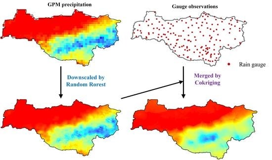
3.2. Downscaling by RF

3.2.1. Downscaling the Satellite Precipitation at the Seasonal Scale

The basic concept of the downscaling algorithm is that the correlation model between precipitation and environmental variables (nighttime land surface temperature (LSTnight), daytime land surface temperature (LSTday), day–night land surface temperature difference (LSTDN), NDVI, elevation, slope, and aspect) is established at a low resolution, and high-resolution environmental variables are then input into the model to obtain high-resolution precipitation. The relationship between environmental variables and precipitation on a daily scale is far less evident than that on annual and monthly scales [25,26]. Considering the time lag of NDVI response to precipitation on a monthly scale, an indirect downscale method was adopted to process the GPM daily precipitation data on a seasonal scale [48]. The GPM precipitation data was downscaled spatially at the seasonal scale, and the seasonal downscaled result was then disaggregated into daily downscaled precipitation.
The original environmental variables, such as nighttime land surface temperature (LSTnight), daytime land surface temperature (LSTday), NDVI, elevation, slope, and aspect, were resampled to 0.01° resolutions and 0.1° resolutions (i.e., NDVI0.01° and NDVI0.1°, LST0.01° and LST0.1°, and DEM0.01° and DEM0.1°) by bilinear interpolation. The time scale of environmental variables and the original GPM daily precipitation were upscaled to the seasonal scale, where the variation of precipitation could be well explained by environmental variables. Data processing was as follows: the GPM daily precipitation was accumulated into the seasonal GPM precipitation (SeasonalGPM), the seasonal average LSTs were calculated by averaging each eight-day LST (SeasonalLST), and the seasonal NDVI (SeasonalNDVI) was calculated by averaging the monthly NDVI. As shown in Figure 3, the detailed steps of the RF-based scale reduction algorithm are as follows:
  • The LSTDN is calculated by subtracting LSTnight from LSTday, and elevation, aspect, and slope data were further extracted from DEM data with ArcGIS software (Esri, Redlands CA, USA).
  • A regression model between the 0.1° environmental variable and 0.1° GPM precipitation data is established by the RF algorithm.
  • The high spatial resolution (0.01°) environmental variable is input into the model established in Step (2), and the 0.01° resolution downscale precipitation (GPM0.01°) is obtained.
  • The 0.1° GPM precipitation (GPMe-0.1°) is estimated using the RF model. The residuals of the models (Res0.1°) are then calculated by subtracting the estimated GPM precipitation (GPMe-0.1°) from the original GPM data (GPMo-0.1°).
  • Subsequently, the residuals of the models (Res0.1°) are spatially interpolated from 0.1° to 0.01° (Res0.01°) using the simple spline function.
  • The corrected downscaled precipitation (GPMc-0.01°) is then obtained by adding the interpolated residual (Res0.01°) to GPM0.01° [49].
After the above steps, the high-resolution seasonal precipitation estimation (Seasonal GPM0.01°) can be obtained.

3.2.2. Disaggregation from Seasonal Precipitation to Daily Precipitation

Finally, we disaggregated the downscaled satellite seasonal precipitation into daily precipitation. Based on the original GPM daily precipitation data, the ratio of daily precipitation to the corresponding seasonal precipitation was obtained. It is assumed that the ratio remains unchanged before and after spatial downscaling [26,48,50]. The RGPMk0.1° is defined by Equation (1):
R G P M k 0.1 ° ( u , s ) = D a i l y G P M k 0.1 ° ( u , s ) S e a s o n a l G P M k 0.1 ° ( u , s )
where k represents the k-th day of a season, u is the spatial location, and s represents the season (spring, summer, autumn, and winter). The RGPMk0.1° was then resampled to 0.01° (RGPMk0.01°) with the bilinear interpolation method, and the downscaled GPM precipitation on the k-th day was acquired by Equation (2):
D a i l y G P M k 0.01 ° ( u , s ) = S e a s o n a l G P M k 0.01 ° ( u , s ) R G P M k 0.01 ° ( u , s )

3.3. Merging by Cokriging

The cokriging (CK) [51] method was applied to merge the downscaled daily precipitation and daily gauge observations [52] by Equation (3):
R * = i = 1 n λ i R g i + j = 1 m α j R i j
where R* represents the estimated precipitation at any location, Rgi (i = 1, 2, 3, …, n) represents gauge observations at different sample locations, and Rrj (j = 1, 2, 3, …, m) represents the downscaled daily precipitation estimates at different sample locations. λi and αj are gauge observations and downscaled daily precipitation weights. The weights are estimated by solving Equation (4):
{ i = 1 n γ ( x i x j ) λ i + j = 1 m γ ( y i x j ) α j + μ 1 = γ ( x 0 x j ) ( i = 1 , 2 , , n ) i = 1 n γ ( x i y j ) λ i + j = 1 m γ ( y i y j ) α j + μ 2 = γ ( x 0 y j ) ( j = 1 , 2 , , m ) i = 1 n λ i = 1 j = 1 m α j = 0
where γ(xixj) is the semivariance between the i-th and j-th primary variables, γ(yixj) is the semivariance between the i-th and j-th secondary variables, γ(xiyj) is the semivariance between the i-th primary variables and j-th secondary variables, γ(x0xj) and γ(x0yj) are the semivariances between the j-th sample points and estimated points, and μ1 and μ2 are the Lagrange parameters. γ(xiyj) is estimated by solving Equation (5):
γ ^ ( h ) = 1 2 N ( h ) i = 1 N ( h ) ( R g ( x i ) R g ( x i + h ) ) × ( R r ( y i ) R r ( y i + h ) )
where γ ^ ( h ) is the value of the variogram at the point, N(h) is the number of pairs of data locations a vector h apart, Rg(xi) is the precipitation from daily gauge observations, and Rr(yi) is the downscaled daily precipitation.
For estimating daily precipitation in this study, we selected the exponential model [53] to construct a theoretical semivariogram model by Equation (6):
γ ( h ) = { c 0 + c ( 1 e h a ) h > 0 0 h = 0
where c0 is the nugget effect, c is the sill, and a is the range.

3.4. Performance Evaluation Indices

In many previous studies, the rain gauge data have been considered as the ‘true rainfall’ to evaluate the accuracy of satellite precipitation datasets [19,20,21,22,23,24,25,26]. This is because rain gauge observations at ground level are able to record rainfall with a lower error rate in comparison with other instruments. In this study, the rain gauge observations were considered as ‘true rainfall’ to evaluate the performance of daily precipitation estimates by quantitative and qualitative indices. The leave-one-out cross validation was adopted to evaluate the merged precipitation estimates [50].

3.4.1. Quantitative Indices

The correlation coefficient (r) reflects the degree of linear correlation between the gauge observations and precipitation estimates, ranging from 0 to 1. The mean absolute error (MAE) represents the absolute errors between the gauge observations and precipitation estimates. The root mean square error (RMSE) represents the sample standard deviation of the difference between the gauge observations and precipitation estimates (called the residual). The Bias represents the deviate degree of the estimations and observations. The modified Kling–Gupta efficiency (KGE) [54] was selected to compare observations with estimations synthetically. A Taylor diagram [55] was drawn to visually show the consistency of the daily precipitation estimates and the gauge observations and to help evaluate the relative accuracy of the daily precipitation estimates.
r = i = 1 n ( p i p ¯ ) ( o i o ¯ ) i = 1 n ( p i p ¯ ) 2 i = 1 n ( o i o ¯ ) 2
M A E = i = 1 n | p i o i | n
R M S E = i = 1 n ( p i o i ) 2 n
Bias = i = 1 n p i i = 1 n o i 1
K G E = 1 ( r 1 ) 2 + ( p ¯ o ¯ 1 ) 2 + ( σ p / p ¯ σ o / 0 1 ) 2
Here, o is the observed precipitation, p is the estimated precipitation, o ¯ is the mean of observed precipitation, p ¯ is the mean of estimated precipitation, σp is the standard deviations of estimated precipitation, and σo is the standard deviations of observed precipitation.

3.4.2. Qualitative Indices

In addition, four qualitative indices—the probability of detection (POD), critical success index (CSI), false alarm ratio (FAR), and frequency bias index (FBI)—were selected to evaluate the ability of daily precipitation estimation to identify precipitation at different precipitation intensities. POD is the correct identification ratio between the satellite precipitation over the number of precipitation events observed by the rain gauges. FAR is the proportion of the precipitation event that the satellite precipitation recognizes while the rain gauges do not recognize. FBI compares the number of precipitation events recognized by satellite precipitation with the number the events recognized by the rain gauges. CSI shows the overall ability of the satellite precipitation to correctly capture the precipitation event.
P O D = H H + M
F A R = F H + F
F B I = H + F H + M
C S I = H H + F + M
Here, H indicates the precipitation events recorded by the rain gauges and the estimated precipitation concurrently, M indicates the precipitation events recorded by the rain gauges but not recorded by the estimated precipitation, and F indicates the precipitation events recorded by the estimated precipitation but not recorded by the rain gauges.

4. Results and Discussion

4.1. Model Regression Performance Analysis

As the core of the downscaling procedure, constructing a downscaling regression model based on the RF algorithm is essential. The RF constructs a downscaling regression model by generating many regression trees and, in this case, utilizing the correlation between GPM precipitation and environmental variables. Therefore, it is essential to probe and describe the relationship accurately, which directly influences the accuracy of the downscaled precipitation results. For the random forest model in this study, the number of trees is the optimized hyperparameter and obtained by the grid search. The depth of the tree used the default value. The number of features was the square root of the total number of features.
Figure 4 shows the correlation between the estimated precipitation by the RF model and the original satellite precipitation at a seasonal scale and the original spatial scale from March 2016 to February 2018. The RF regression model used for downscaling performed well in the four seasons. The precipitation estimates had a good correlation with the original precipitation data, with little difference. The r value was between 0.98 and 0.99, the bias was between 0.01% and 0.07%. As shown in Figure 4, higher precipitation results in lower bias, especially for Figure 4c. The model performance was less influenced by seasonal variation, indicating that the significant interrelationship between seasonal GPM precipitation and seasonal environmental variables (LSTnight, LSTday, LSTDN, NDVI, elevation, slope, and aspect) was relatively steady at 0.1° resolutions, which ensures the accuracy of the spatial downscaling.

4.2. Performance of the Merged Precipitation

Figure 5 shows the spatial precipitation distribution patterns on Days 122, 219, and 290 in 2017 from the original GPM precipitation (Ori_GPM), the downscaled GPM precipitation (Down_GPM), and the merged precipitation by CK (DM_CK). Generally, the precipitation spatial distribution of Ori_GPM is like a mosaic because of its coarse resolution, and the spatial distribution details of the precipitation are insufficient. Compared with Ori_GPM, Down_GPM dramatically improves the precipitation spatial detail and retains the spatial precipitation distribution patterns in the aforementioned days.
The daily precipitation estimates from Down_GPM were clearly corrected after merging with the gauge observations, which led to some differences between Down_GPM and DM_CK. The merging corrected the daily precipitation amounts of Down_GPM, which is evident for the precipitation on the 122nd day of 2017. The merging result decreased the precipitation noticeably in the southwest of the study area, while the northwest precipitation increased significantly. The reason is that satellite observations overestimated the precipitation in the southwest and underestimated the precipitation in the northwest. From the above three daily precipitation measurements, it can be seen that the merging precipitation (DM_CK) not only corrected the daily precipitation amounts and improved the accuracy of downscaling precipitation (Down_GPM) but also basically retained the original GPM precipitation (Ori_GPM) spatial distribution pattern.

4.3. Evaluations

To evaluate the accuracy of CK merging precipitation estimation, five evaluation indices (r, Bias, MAE, RMSE, and KGE) were used to evaluate the accuracy. In Section 4.3.1, the evaluation process was carried out on the gridded spatial scale for daily and monthly timescales, respectively. In Section 4.3.2, the evaluation process was carried out on the basin spatial scale for daily and monthly timescales, respectively.

4.3.1. Evaluation on a Gridded Scale

The Ori_GPM, Down_GPM, and DM_CK from March 2016 to February 2018 were evaluated. Table 2 shows the general performance of the three precipitation datasets, and DM_CK performs best. Compared with Ori_GPM, the r and the KGE values of DM_CK increased by 25.00% and 29.82%, and the values of Bias, MAE, and RMSE decreased by 78.89%, 36.09%, and 26.40%, respectively. Although the performance of spatial detail of DM_CK is dramatically improved compared with that of Ori_GPM (Figure 5), the evaluation indices of the two daily precipitation estimates are almost the same during the whole study period, with only Bias reduced by 16.63%. The reason is that there is no additional valid precipitation observation in the downscaling process. The accuracy of Down_GPM was improved remarkably after merging with the gauge observations, which significantly decreased the Bias, MAE, and RMSE, and increased the r and the KGE.
As shown in Figure 6, some specific rainfall events were selected to evaluate three daily precipitation datasets in estimating daily precipitation. The rainfall events were determined according to the division of flood events based on hydrological hydrographs observed at the outlet streamflow gauge of the study area. The seven selected rainfall events and some statistics are listed in Table 3. The selected rainfall events were distributed from May to October, spanning the three seasons of spring, summer, and autumn, which include the main rainfall seasons in the Hanjiang River Basin. Among the seven selected rainfall events, Down_GPM and Ori_GPM had similar performance in estimating daily precipitation, while DM_CK had the optimum accuracy in the three datasets (Figure 6).
To compare the accuracy of precipitation estimation more intuitively, Taylor diagrams of the three daily precipitation estimates and the gauge observations and the accumulated monthly precipitation estimates were drawn. The closer the point is to the gauge observations, the higher the accuracy is. As shown in Figure 7, DM_CK has the highest accuracy, while Ori_GPM and Down_GPM have similar performance.
The performance of the Ori_GPM, Down_GPM, and DM_CK were also evaluated for the various precipitation intensities, as shown in Figure 8. For identifying rainfall events, the three precipitation datasets had the same change regularities. The three precipitation datasets identified no-rain events well, but the identification ability gradually decreased with the increase of precipitation. The identification performance of Down_GPM was practically identical to that of Ori_GPM for each various precipitation intensity. The DM_CK remarkably enhanced the ability to identify rain events. Except for the last three precipitation intensities (30~40, 40~50, and >50 mm) of the evaluation index FBI, the detection ability of other precipitation intensities was significantly improved.
As the amount of precipitation increased, RMSEs and MAEs of three daily precipitation datasets gradually increased and had similar variation patterns. The RMSEs and MAEs of the merged precipitation dataset (DM_CK) were smaller than those of the other two precipitation datasets in the various precipitation intensities, indicating that the accuracy of DM_CK was significantly improved.
In addition, the abilities of the three daily precipitation datasets were verified to capture the time series variation of the daily precipitation at the gauge positions, as shown in Figure 9. Among the three daily precipitation datasets, Down_GPM and Ori_GPM had a similar ability to capture the time series variation of daily precipitation. For DM_CK compared with the other two kinds of precipitation, r was improved, and MAE and RMSE were decreased, which indicated that the merged results could capture the time series variation of daily precipitation well and remarkably enhanced the temporal uniformity between the gauge observations and daily precipitation datasets.
The three monthly precipitation estimates from March 2016 to February 2018 were evaluated. Table 4 and Figure 10 show the overall performance of the three precipitation datasets and the variation of evaluation indices with time, respectively. The monthly precipitation estimates from Down_GPM had a similar performance to those from Ori_GPM. Among the three precipitation datasets, the DM_CK had the optimum accuracy for estimating the monthly precipitation. Compared with Ori_GPM, the merged precipitation noticeably improved the accuracy for estimating the monthly precipitation, reducing RMSE and MAE by 12.53% and 19.94%, respectively. However, the improvement was less than those at the daily time scale. In addition, these improvements are volatile over time; in some months, the accuracy actually decreased. For example, although the r of monthly precipitation estimates in February 2017 had increased, MAE and RMSE had increased (Figure 10). These results are caused by two reasons. First, the daily precipitation was accumulated into monthly precipitation, which offset the accuracy improvement on the daily time scale to some extent. Second, a low correlation between the downscaling precipitation estimates (Down_GPM) and the gauge observations may lead to errors when using cokriging for merging process, resulting in a decrease in DM_CK accuracy.

4.3.2. Evaluation on the Basin Scale

The performance of the three precipitation datasets in estimating the basin average daily precipitation (BADP) was shown in Figure 11. Ori_GPM and Down_GPM overestimated the BADP by less than 15 mm and underestimated BADP by more than 15 mm. For the three statistical indices, no significant difference was found between Ori_GPM and Down_GPM, indicating similar performances in estimating BADP. Compared with Ori_GPM, the accuracy of the merged precipitation had been significantly improved, reducing its RMSE and MAE by 90.46% and 93.08%, respectively (Table 5). Compared to Ori_GPM, the merged precipitation was close to the 1:1 line, indicating that it had optimal consistency with the gauge observations.
As shown in Figure 11, for estimating the basin average monthly precipitation (BAMP), the three daily precipitation datasets had a higher consistency with the gauge observations than the estimation of BADP. This is especially the case for both Ori_GPM and Down_TRMM, where the r increased from 0.87 to more than 0.98. The reason is that the positive and negative errors will counteract each other in the process of daily precipitation, accumulating into monthly precipitation. Ori_GPM and Down_GPM overestimated the most precipitation on the monthly scale. Consistent with this, the performance of Ori_GPM was nearly equivalent to Down_GPM, and the merged precipitation had a better performance than Down_GPM. Compared with Ori_GPM, the accuracy of DM_CK was significantly improved. The MAE and RMSE were reduced by 84.13% and 81.68%, respectively (Table 5). The accuracy improvement of BAMP was less than that of BADP.
Table 6 further assesses the performances of the three daily precipitation datasets in detecting rainless events of RADP. Ori_GPM and Down_GPM had the same ability to detect rainless events. Compared with Ori_GPM, DM_CK had significantly improved the ability to identify no-rain events, with a POD of 1.

4.4. Discussion

Compared with previous studies [22,23,26], which only use one or two environmental variables (NDVI and DEM), the six environmental variables (LSTnight, LSTday, LSTDN, NDVI, elevation, slope, and aspect) were adopted to construct the RF downscaling regression model in this study. The response relationship between vegetation and precipitation has been widely discussed [56,57,58]. The distribution of vegetation types on the underlying surface can affect the latent heat flux into the atmosphere, which will significantly affect the humidity of the lower atmosphere, thereby affecting the development of moist convection [6]. The response relationship between precipitation and vegetation usually lags 2–3 months [59,60,61], so this study established the relationship between precipitation and vegetation on a seasonal scale. In this study, the land surface temperature was introduced as environmental variables to downscale GPM precipitation. Trenberth et al. [62] found the covariability between precipitation and surface temperature on a global scale. Over land, there is a negative correlation between surface temperature and precipitation in general [62]. Evaporation on the wet ground is likely to bring away part of the energy, resulting in a drop in temperature. Moreover, the clouds will also block the sun, reducing the energy provided on the ground and causing the temperature to drop further. Thus, the precipitation–LST relationship is adopted for downscaling the satellite precipitation [21,24]. The DEM is widely used for downscaling the satellite precipitation [19,20,21,22]. As the elevation increases, due to the uplifting effect of the terrain, the air mass will rise and expand, thereby increasing the humidity of the air mass to form precipitation [63]. In addition, slope and aspect are related to the prevailing wind orientation, determining the potential relative excess or deficiency of moisture [64].
Therefore, using these six variables can describe the relationship between environmental factors and rainfall from different perspectives compared to studies [22,23,26] only using one or two variables, which will help to build a more accurate regression downscaling model. As shown in Figure 4, the RF regression model constructed from the proposed six environmental variables and precipitation has a high accuracy of estimating precipitation and can be used in the downscaling process. Compared with the original GPM precipitation, the accuracy of downscaled GPM precipitation is guaranteed (Table 2, Table 4, Table 5 and Table 6).
In this study, the daily satellite precipitation data is from the GPM_3IMERGDF, derived from the half-hourly GPM_3IMERGHH (GPM IMERG Final Precipitation L3 Half Hourly 0.1° × 0.1° V06). The GPM_3IMERGHH combines the multi-satellite data for the month with GPCC (Global Precipitation Climatology Centre) gauge analysis for month-to-month adjustment. The GPCC provides gridded gauge analysis products, including the different spatial resolutions of 0.5°, 1°, and 2.5°. In this study, the gauge data were collected in 160 daily rain gauges from the Hanjiang Bureau of Yangtze River Commission of Hubei Province. The sources of these two types of gauge data are different. Therefore, the errors from the gauge data applied in the GPM_3IMERGDF do not need to be considered in this study.
Data fusion refers to the process of fusing data from multiple sources to obtain more accurate and valuable information than any single data source [65]. Traditional rain gauges can provide relatively accurate rainfall values on the point scales, but they are not accurate for estimating continuous spatial precipitation distributions on a large scale [10]. The satellite precipitation observation data provides reliable precipitation estimates and reflects more spatial distributions than the rain gauge data, but their accuracy is limited. Therefore, combining the advantages of gauge observations and satellite precipitation observations, fusing the observation information of the two to obtain a reasonable precipitation estimate for the study area is worth studying.
In the previous studies, Chen et al. [66] employed area-to-point kriging (ATPK) for downscaling the monthly TRMM product, then integrating the downscaled precipitation with the gauge observations using geographically weighted regression kriging (GWRK). Chen et al. [48] downscaled the TRMM precipitation by geographically weighted regression (GWR) then used kriging with external drift (KED) to fuse the downscaled TRMM precipitation with gauge observations. Chen et al. [50] used geographically weighted ridge regression (GWRR) to fuse four downscaled satellite precipitation by GWR with gauge observations. This study introduced the random forest model from machine learning algorithms and the cokriging method in geostatistics to construct a downscaling– merging scheme. Compared with previous downscaling algorithms such as GWR, the random forest model is not sensitive to multivariate collinearity and can handle high-dimensional data without dimensionality reduction. Therefore, in the downscaling process, the random forest model does not need to consider the collinearity between environmental variables and eliminates high-dimensional data (multiple environmental variables) processing. Cokriging was first employed for the fusion of radar rainfall data and gauge observations data [52]. In this study, it was proved to be suitable for the fusion of downscaled satellite precipitation data and gauge observations data. The results show that the accuracy of the fusion precipitation product has been significantly improved (Table 2, Table 4, Table 5 and Table 6).
For the fusion of satellite precipitation and gauge observation, increasing the distribution density of gauges is conducive to improving the fusion results quality [66,67,68]. Nevertheless, this improvement will be limited when the gauge density reaches a critical threshold [30]. Concerning the various fusion algorithms, the optimal gauge density is different for the optimal fusion results, worthy of further study.

5. Conclusions

In this study, a downscaling–merging scheme was used to merge the downscaled results with gauge observations to obtain high-resolution and high-quality daily precipitation datasets within a specific range. In the downscaling process, the RF regression model was employed to establish a statistical downscaling model. The cokriging method was used to merge the gauge observations with the downscaling precipitation results. Taking the Danjiangkou Reservoir in the Hanjiang River Basin as the study area, the feasibility of this method was verified by using the GPM daily precipitation data and the gauge observations from 1 March 2016 to 28 February 2018. According to the research results, the following conclusions were drawn:
  • The downscaling–merging scheme can efficiently generate high-resolution (0.01°) and high-quality daily precipitation datasets over a large scale.
  • The RF downscaling model established on a seasonal scale can accurately reflect the correlation between GPM precipitation and environmental variables, and the regression relationship is relatively stable. The downscaling daily precipitation datasets not only preserved the original spatial distribution pattern of satellite precipitation data but also significantly improved their spatial details.
  • The downscaling daily precipitation data based on the RF model improved the spatial resolution of the original GPM daily precipitation data and had almost the same accuracy as the original GPM daily precipitation data.
  • After the merging process, the accuracy of Down_GPM was significantly improved, MAE and RMSE were reduced by 36.09% and 26.40% respectively, and the detection ability of precipitation events was also improved.
In summary, the proposed downscaling–merging scheme based on RF and cokriging can successfully improve the spatial resolution and accuracy of daily precipitation estimation. In the future, studies should strive to obtain high-resolution precipitation datasets at higher time resolutions (hourly or subhourly) to adapt to more application scenarios.

Author Contributions

Conceptualization, X.Y., H.C., and S.S.; Methodology, X.Y., H.C., and B.T.; Supervision, X.Y., H.C., and J.-S.K.; Validation, X.Y, H.C., and S.S.; Formal Analysis, X.Y., B.T., and J.W.; Investigation, X.Y., B.T., and S.S.; Data Curation, J.W; Writing—Original Draft Preparation, X.Y.; Writing—Review and Editing, H.C. and J.-S.K.; Funding Acquisition, J.W. All authors have read and agreed to the published version of the manuscript.

Funding

This research was funded by National Key Research and Development Program (2019YFC1510703).

Conflicts of Interest

The authors declare no conflict of interest.

References

  1. Jesus, M.D.; Rinaldo, A.; Rodriguez-Iturbe, I. Point rainfall statistics for ecohydrological analyses derived from satellite integrated rainfall measurements. Water Resour. Res. 2015, 51, 2974–2985. [Google Scholar] [CrossRef] [Green Version]
  2. Long, Y.; Zhang, Y.; Ma, Q. A Merging Framework for Rainfall Estimation at High Spatiotemporal Resolution for Distributed Hydrological Modeling in a Data-Scarce Area. Remote Sens. 2016, 8, 599. [Google Scholar] [CrossRef] [Green Version]
  3. Zhang, S.; Gao, H.; Naz, B.S. Monitoring reservoir storage in South Asia from multisatellite remote sensing. Water Resour. Res. 2015, 50, 8927–8943. [Google Scholar] [CrossRef]
  4. Goodrich, D.C.; Faurès, J.M.; Woolhiser, D.A.; Lane, L.J.; Sorooshian, S. Measurement and analysis of small-scale con-vective storm rainfall variability. J. Hydrol. 1995, 173, 283–308. [Google Scholar] [CrossRef]
  5. Ahmad, S.; Kalra, A.; Stephen, H. Estimating soil moisture using remote sensing data: A machine learning approach. Adv. Water Resour. 2010, 33, 69–80. [Google Scholar] [CrossRef]
  6. Spracklen, D.V.; Arnold, S.R.; Taylor, C.M. Observations of increased tropical rainfall preceded by air passage over forests. Nature 2012, 489, 282–285. [Google Scholar] [CrossRef] [PubMed]
  7. Song, Y.; Liu, H.; Wang, X.; Zhang, N.; Sun, J. Numerical simulation of the impact of urban non-uniformity on precipitation. Adv. Atmos. Sci. 2016, 33, 783–793. [Google Scholar] [CrossRef]
  8. Syed, T.H.; Lakshmi, V.; Paleologos, E.; Lohmann, D.; Mitchell, K.; Famiglietti, J.S. Analysis of process controls in land surface hydrological cycle over the continental United States. J. Geophys. Res. Atmos. 2004, 109, D22105. [Google Scholar] [CrossRef] [Green Version]
  9. Gebregiorgis, A.S.; Hossain, F. Understanding the Dependence of Satellite Rainfall Uncertainty on Topography and Climate for Hydrologic Model Simulation. IEEE Trans. Geosci. Remote Sens. 2013, 51, 704–718. [Google Scholar] [CrossRef]
  10. Javanmard, S.; Yatagai, A.; Nodzu, M.I.; Bodaghjamali, J.; Kawamoto, H. Comparing high-resolution gridded precipitation data with satellite rainfall estimates of TRMM_3B42 over Iran. Adv. Geosci. 2010, 25, 119–125. [Google Scholar] [CrossRef] [Green Version]
  11. Villarini, G.; Krajewski, W.F. Review of the Different Sources of Uncertainty in Single Polarization Radar-Based Estimates of Rainfall. Surv. Geophys. 2009, 31, 107–129. [Google Scholar] [CrossRef]
  12. Kummerow, C.; Simpson, J.; Thiele, O.; Barnes, W.; Chang, A.; Stocker, E.; Adler, R.F.; Hou, A.; Kakar, R.; Wentz, F.; et al. The status of the Tropical Rainfall Measuring Mission (TRMM) after two years in orbit. J. Appl. Meteorol. 2000, 39, 1965–1982. [Google Scholar] [CrossRef]
  13. Kubota, T.; Shige, S.; Hashizume, H.; Aonashi, K.; Takahashi, N.; Seto, S.; Hirose, M.; Takayabu, Y.N.; Ushio, T.; Nakagawa, K. Global Precipitation Map Using Satellite-Borne Microwave Radiometers by the GSMaP Project: Production and Validation. IEEE Trans. Geosci. Remote Sens. 2007, 45, 2259–2275. [Google Scholar] [CrossRef]
  14. Huffman, G.J.; Adler, R.F.; Arkin, P.; Chang, A.; Ferraro, R.; Gruber, A.; Janowiak, J.; McNab, A.; Rudolf, B.; Schneider, U. The global precipitation climatology project (GPCP) combined precipitation dataset. Bull. Am. Meteorol. Soc. 1997, 78, 5–20. [Google Scholar] [CrossRef]
  15. Skofronick-Jackson, G.; Petersen, W.A.; Berg, W.; Kidd, C.; Stocker, E.F.; Kirschbaum, D.B.; Kakar, R.; Braun, S.A.; Huffman, G.J.; Iguchi, T.; et al. The Global Precipitation Measurement (GPM) mission for science and society. Bull. Am. Meteorol. Soc. 2017, 98, 1679–1695. [Google Scholar] [CrossRef]
  16. Sorooshian, S.; Aghakouchak, A.; Arkin, P.; Eylander, J.; Foufoula-Georgiou, E.; Harmon, R.; Hendrickx, J.; Imam, B.; Kuligowski, R.; Skahill, B. Advanced Concepts on Remote Sensing of Precipitation at Multiple Scales. Bull. Am. Meteorol. Soc. 2011, 92, 1353–1357. [Google Scholar] [CrossRef]
  17. Rummukainen, M. State-of-the-art with regional climate model. Wiley Interdiscip. Rev. Clim. Chang. 2010, 1, 82–96. [Google Scholar] [CrossRef]
  18. Immerzeel, W.W.; Rutten, M.M.; Droogers, P. Spatial downscaling of TRMM precipitation using vegetative response on the Iberian Peninsula. Remote Sens. Environ. 2009, 113, 362–370. [Google Scholar] [CrossRef]
  19. Jia, S.; Zhu, W.; Aifeng, L.; Yan, T. A statistical spatial downscaling algorithm of TRMM precipitation based on NDVI and DEM in the Qaidam Basin of China. Remote Sens. Environ. 2011, 115, 3069–3079. [Google Scholar] [CrossRef]
  20. Fang, J.; Du, J.; Xu, W.; Shi, P.; Li, M.; Ming, X. Spatial downscaling of TRMM precipitation data based on the orographical effect and meteorological conditions in a mountainous area. Adv. Water Resour. 2013, 61, 42–50. [Google Scholar] [CrossRef]
  21. Jing, W.; Yang, Y.; Yue, X.; Zhao, X. A Spatial Downscaling Algorithm for Satellite-Based Precipitation over the Tibetan Plateau Based on NDVI, DEM, and Land Surface Temperature. Remote Sens. 2016, 8, 655. [Google Scholar] [CrossRef] [Green Version]
  22. Zhan, C.; Jian, H.; Shi, H.; Liu, L.; Dong, Y. Spatial Downscaling of GPM Annual and Monthly Precipitation Using Regression-Based Algorithms in a Mountainous Area. Adv. Meteorol. 2018, 2018, 1–13. [Google Scholar] [CrossRef] [Green Version]
  23. Zhang, J.; Fan, H.; He, D.; Chen, J. Integrating precipitation zoning with random forest regression for the spatial downscaling of satellite-based precipitation: A case study of the Lancang—Mekong River basin. Int. J. Clim. 2019, 39, 3947–3961. [Google Scholar] [CrossRef]
  24. Ma, Z.; He, K.; Tan, X.; Xu, J.; Fang, W.; He, Y.; Hong, Y. Comparisons of spatially downscaling TMPA and IMERG over the Tibetan Plateau. Remote Sens. 2018, 10, 1883. [Google Scholar] [CrossRef] [Green Version]
  25. Ma, Z.; He, K.; Tan, X.; Liu, Y.; Lu, H.; Shi, Z. A new approach for obtaining precipitation estimates with a finer spatial resolution on a daily scale based on TMPA V7 data over the Tibetan Plateau. Int. J. Remote Sens. 2019, 40, 8465–8483. [Google Scholar] [CrossRef]
  26. Chen, F.; Gao, Y.; Wang, Y.; Qin, F.; Li, X. Downscaling satellite-derived daily precipitation products with an integrated framework. Int. J. Climatol. A J. R. Meteorol. Soc. 2019, 39, 1287–1304. [Google Scholar] [CrossRef]
  27. Sun, Q.; Miao, C.; Duan, Q.; Ashouri, H.; Sorooshian, S.; Hsu, K. A review of global precipitation data sets: Data sources, estimation, and intercomparisons. Rev. Geophys. 2018, 56, 79–107. [Google Scholar] [CrossRef] [Green Version]
  28. Katiraie-Boroujerdy, P.; Asanjan, A.A.; Hsu, K.; Sorooshian, S. Intercomparison of PERSIANN-CDR and TRMM-3B42V7 precipitation estimates at monthly and daily time scales. Atmos. Res. 2017, 193, 36–49. [Google Scholar] [CrossRef] [Green Version]
  29. Beck, H.E.; Wood, E.F.; Pan, M.; Fisher, C.K.; Miralles, D.G.; Van Dijk, A.I.; McVicar, T.R.; Adler, R.F. MSWEP V2 global 3-hourly 0.1 precipitation: Methodology and quantitative assessment. Bull. Am. Meteorol. Soc. 2019, 100, 473–500. [Google Scholar] [CrossRef] [Green Version]
  30. Yang, Z.; Hsu, K.; Sorooshian, S.; Xu, X.; Braithwaite, D.; Zhang, Y.; Verbist, K.M. Merging high-resolution satellite-based precipitation fields and point-scale rain gauge measurements—A case study in Chile. J. Geophys. Res. Atmos. 2017, 122, 5267–5284. [Google Scholar] [CrossRef]
  31. Baez-Villanueva, O.M.; Zambrano-Bigiarini, M.; Beck, H.E.; McNamara, I.; Ribbe, L.; Nauditt, A.; Birkel, C.; Verbist, K.; Giraldo-Osorio, J.D.; Thinh, N.X. RF-MEP: A novel Random Forest method for merging gridded precipitation products and ground-based measurements. Remote Sens. Environ. 2020, 239, 111606. [Google Scholar] [CrossRef]
  32. Cheema, M.J.M.; Bastiaanssen, W.G.M. Local calibration of remotely sensed rainfall from the TRMM satellite for different periods and spatial scales in the Indus Basin. Int. J. Remote Sens. 2012, 33, 2603–2627. [Google Scholar] [CrossRef]
  33. Manz, B.; Buytaert, W.; Zulkafli, Z.; Lavado, W.; Willems, B.; Robles, L.A.; Rodr, I.; Guez-S, A.; Nchez, J. High-resolution satellite-gauge merged precipitation climatologies of the Tropical Andes. J. Geophys. Res. Atmos. 2016, 121, 1190–1207. [Google Scholar] [CrossRef] [Green Version]
  34. Hou, A.Y.; Kakar, R.K.; Neeck, S.; Azarbarzin, A.A.; Kummerow, C.D.; Kojima, M.; Oki, R.; Nakamura, K.; Iguchi, T. The Global Precipitation Measurement Mission. Bull. Am. Meteorol. Soc. 2013, 95, 701–722. [Google Scholar] [CrossRef]
  35. Huffman, G.J.; Bolvin, D.T.; Braithwaite, D.; Hsu, K.; Joyce, R.; Xie, P.; Yoo, S. NASA global precipitation measurement (GPM) integrated multi-satellite retrievals for GPM (IMERG). Algorithm Theoretical Basis Doc. (ATBD) Vers. 2015, 4, 26. [Google Scholar]
  36. Huffman, G.J.; Bolvin, D.T.; Nelkin, E.J. Integrated Multi-satellitE Retrievals for GPM (IMERG) technical documentation. NASA/GSFC Code 2015, 612, 2019. [Google Scholar]
  37. Breiman, L. Bagging Predictors. Mach. Learn. 1996, 24, 123–140. [Google Scholar] [CrossRef] [Green Version]
  38. Breiman, L. Random forests. Mach. Learn. 2001, 45, 5–32. [Google Scholar] [CrossRef] [Green Version]
  39. Cutler, A.; Cutler, D.R.; Stevens, J.R. Random forests. In Ensemble Machine Learning; Springer: Berlin/Heidelberg, Germany, 2012; pp. 157–175. [Google Scholar]
  40. Chaney, N.W.; Wood, E.F.; Mcbratney, A.B.; Hempel, J.W.; Nauman, T.W.; Brungard, C.W.; Odgers, N.P. POLARIS: A 30-meter probabilistic soil series map of the contiguous United States. Geoderma 2016, 274, 54–67. [Google Scholar] [CrossRef] [Green Version]
  41. Zhao, T.; Yang, D.; Cai, X.; Cao, Y. Predict seasonal low flows in the upper Yangtze River using random forests model. J. Hydroelectr. Eng. 2012, 31, 18–24. [Google Scholar]
  42. He, X.; Zhao, T.; Yang, D. Prediction of monthly inflow to the Danjiangkou reservoir by distributed hydrological model and hydro-climatic teleconnections. J. Hydroelectr. Eng. 2013, 32, 4–9. [Google Scholar]
  43. Carlisle, D.M.; Falcone, J.; Wolock, D.M.; Meador, M.R.; Norrjs, R.H. Predicting the natural flow regime: Models for assessing hydrological alteration in streams. River Res. Appl. 2010, 26, 118–136. [Google Scholar] [CrossRef]
  44. Peters, J.; Baets, B.D.; Verhoest, N.; Samson, R.; Degroeve, S.; Becker, P.D.; Huybrechts, W. Random forests as a tool for ecohydrological distribution modelling. Ecol. Model. 2007, 207, 304–318. [Google Scholar] [CrossRef]
  45. Liaw, A.; Wiener, M. Classification and regression by random forest. R News 2002, 2, 18–22. [Google Scholar]
  46. Ibarra-Berastegi, G.; Saénz, J.; Ezcurra, A.; Elías, A.; Diaz Argandoña, J.; Errasti, I. Downscaling of surface moisture flux and precipitation in the Ebro Valley (Spain) using analogues and analogues followed by random forests and multiple linear regression. Hydrol. Earth Syst. Sc. 2011, 15, 1895–1907. [Google Scholar] [CrossRef]
  47. Swami, A.; Jain, R. Scikit-learn: Machine Learning in Python. J. Mach. Learn. Res. 2013, 12, 2825–2830. [Google Scholar]
  48. Chen, F.; Gao, Y.; Wang, Y.; Li, X. A downscaling-merging method for high-resolution daily precipitation estimation. J. Hydrol. 2020, 581, 124414. [Google Scholar] [CrossRef]
  49. Yuli, S.; Lei, S.; Zhen, X.; Yurong, L.; Myneni, R.B.; Sungho, C.; Lin, W.; Xiliang, N.; Cailian, L.; Fengkai, Y.; et al. Mapping Annual Precipitation across Mainland China in the Period 2001–2010 from TRMM3B43 Product Using Spatial Downscaling Approach. Remote Sens. 2015, 7, 5849–5878. [Google Scholar]
  50. Chen, S.; Xiong, L.; Ma, Q.; Kim, J.; Chen, J.; Xu, C. Improving daily spatial precipitation estimates by merging gauge observation with multiple satellite-based precipitation products based on the geographically weighted ridge regression method. J. Hydrol. 2020, 589, 125156. [Google Scholar] [CrossRef]
  51. Sun, X.; Mein, R.G.; Keenan, T.D.; Elliott, J.F. Flood estimation using radar and raingauge data. J. Hydrol. 2000, 239, 4–18. [Google Scholar] [CrossRef]
  52. Wang, Q.; Xu, C.; Chen, H. Comparison and Analysis of Different Variogram Functions Models in Kriging Interpolation of Daily Rainfall. J. Water Resour. Res. 2016, 5, 469–477. [Google Scholar] [CrossRef]
  53. Goovaerts, P. Geostatistics for Natural Resources Evaluation; Oxford University Press on Demand: Oxford, UK, 1997. [Google Scholar]
  54. Kling, H.; Fuchs, M.; Paulin, M. Runoff conditions in the upper Danube basin under an ensemble of climate change scenarios. J. Hydrol. 2012, 424, 264–277. [Google Scholar] [CrossRef]
  55. Taylor, K.E. Summarizing multiple aspects of model performance in a single diagram. J. Geophys. Res. Atmos. 2001, 106, 7183–7192. [Google Scholar] [CrossRef]
  56. Wang, J.; Price, K.P.; Rich, P.M. Spatial patterns of NDVI in response to precipitation and temperature in the central Great Plains. Int. J. Remote Sens. 2001, 22, 3827–3844. [Google Scholar] [CrossRef]
  57. Zhang, X.; Friedl, M.A.; Scha Af, C.B.; Strahler, A.H.; Zhong, L. Monitoring the response of vegetation phenology to precipitation in Africa by coupling MODIS and TRMM instruments. J. Geophys. Res. Atmos. 2005, 110, D12. [Google Scholar] [CrossRef]
  58. Vicente-Serrano, S.M.; Gouveia, C.; Camarero, J.J.; Beguería, S.; Sanchez-Lorenzo, A. Response of vegetation to drought time-scales across global land biomes. Proc. Natl. Acad. Sci. USA 2012, 110, 52–57. [Google Scholar] [CrossRef] [PubMed] [Green Version]
  59. Brunsell, N.A. Characterization of land-surface precipitation feedback regimes with remote sensing. Remote Sens. Environ. 2006, 100, 200–211. [Google Scholar] [CrossRef]
  60. Ji, L.; Peters, A.J. Lag and Seasonality Considerations in Evaluating AVHRR NDVI Response to Precipitation. Photogramm. Eng. Remote Sens. 2005, 71, 1053–1061. [Google Scholar] [CrossRef]
  61. Wang, J.; Rich, P.M.; Price, K.P. Temporal responses of NDVI to precipitation and temperature in the central Great Plains, USA. Int. J. Remote Sens. 2003, 24, 2345–2364. [Google Scholar] [CrossRef]
  62. Trenberth, K.E.; Shea, D.J. Relationships between precipitation and surface temperature. Geophys. Res. Lett. 2005, 32, 14. [Google Scholar] [CrossRef]
  63. Sokol, Z.; Bliznak, V. Areal distribution and precipitation–altitude relationship of heavy short-term precipitation in the Czech Republic in the warm part of the year. Atmos. Res. 2009, 94, 652–662. [Google Scholar] [CrossRef]
  64. Badas, M.G.; Deidda, R.; Piga, E. Orographic influences in rainfall downscaling. Adv. Geosci. 2005, 2, 285–292. [Google Scholar] [CrossRef] [Green Version]
  65. Wald, L. Some terms of reference in data fusion. IEEE Trans. Geosci. Remote 2002, 37, 1190–1193. [Google Scholar] [CrossRef] [Green Version]
  66. Chena, Y.; Huanga, J.; Sheng, D.S.; Mansaraya, L.R.; Wangh, X. A new downscaling-integration framework for high-resolution monthly precipitation estimates: Combining rain gauge observations, satellite-derived precipitation data and geographical ancillary data. Remote Sens. Environ. 2018, 214, 154–172. [Google Scholar] [CrossRef]
  67. Li, H.; Hong, Y.; Xie, P.; Gao, J.; Niu, Z.; Kirstetter, P.; Yong, B. Variational merged of hourly gauge-satellite precipitation in China: Preliminary results. J. Geophys. Res. Atmos. 2015, 120, 9897–9915. [Google Scholar] [CrossRef]
  68. Park, N.W.; Kyriakidis, P.; Hong, S. Geostatistical Integration of Coarse Resolution Satellite Precipitation Products and Rain Gauge Data to Map Precipitation at Fine Spatial Resolutions. Remote Sens. 2017, 9, 255. [Google Scholar] [CrossRef] [Green Version]
Figure 1. Study area and the location of rain gauges.
Remotesensing 13 02040 g001
Figure 2. Diagram of the random forest (RF) algorithm.
Remotesensing 13 02040 g002
Figure 3. Flowchart of the two-step downscaling–merging scheme based on RF and cokriging.
Remotesensing 13 02040 g003
Figure 4. Scatter plots (the color bar represented the density of the point distribution) of the original satellite precipitation and the predicted precipitation by the RF model at original spatial scale and seasonal for (a) Spring, (b) Summer, (c) Autumn, and (d) Winter.
Remotesensing 13 02040 g004
Figure 5. Precipitation maps of Ori_GPM: the original GPM precipitation, Down_GPM: the downscaled GPM precipitation and DM_CK: the merged precipitation by CK on Days 122, 219, and 290 in 2017.
Remotesensing 13 02040 g005
Figure 6. Evaluation for quantitative indices for the Ori_GPM; Down_GPM and DM_CK at the specific rainfall events.
Remotesensing 13 02040 g006
Figure 7. Taylor diagrams for daily precipitation and monthly precipitation of the gauge observation, Ori_GPM, Down_GPM, and DM_CK across the entire period from March 2016 to February 2018.
Remotesensing 13 02040 g007
Figure 8. Evaluation for qualitative indices and quantitative indices of the Ori_GPM, Down_GPM, and DM_CK for daily precipitation estimates in various precipitation intensity from March 2016 to February 2018.
Remotesensing 13 02040 g008
Figure 9. Evaluation for quantitative indices of the Ori_GPM, Down_GPM, and DM_CK for daily precipitation estimates at gauge positions from March 2016 to February 2018.
Remotesensing 13 02040 g009
Figure 10. Evaluation for quantitative indices of the Ori_GPM, Down_GPM, and DM_CK for monthly precipitation estimates with the time variation from March 2016 to February 2018.
Remotesensing 13 02040 g010
Figure 11. Scatterplots of BADP: basin average daily precipitation (a) and BAMP: basin average monthly precipitation (b) from the Ori_GPM, Down_GPM, and DM_CK against the gauge observations from March 2016 to February 2018.
Remotesensing 13 02040 g011
Table 1. All the image products used in the study.
Image ProductsDatasetResolutionLatency
PrecipitationGPM_3IMERGDFDaily, 0.1°3.5 months
NDVI 1MOD13A3Monthly, 1 km1 month
LST 2MOD11A28-day, 1 km8 days
DEM 3SRTM-, 90 m-
1 NDVI: normalized vegetation index; 2 LST: land surface temperature; 3 DEM: digital elevation model.
Table 2. Evaluation for quantitative indices of the Ori_GPM, Down_GPM, and DM_CK for daily precipitation estimates from March 2016 to February 2018.
Titler 4TitleBiasTitleMAE 5TitleRMSE 6TitleKGE 7Title
ValueIM 8 (%)Value (%)IM (%)Value (mm)IM (%)Value (mm)IM (%)ValueIM (%)
Ori_GPM 10.64015.51%02.3206.1700.560
Down_GPM 20.64012.93%−16.63%2.30−0.86%6.06−1.78%0.571.79%
DM_CK 30.8025.00%2.73%−78.89%1.47−36.09%4.46−26.40%0.7429.82%
1 Ori_GPM: the original GPM precipitation; 2 Down_GPM: the downscaled GPM precipitation; 3 DM_CK: the merged precipitation by CK; 4 r: correlation coefficient; 5 MAE: mean absolute error; 6 RMSE: root mean square error; 7 KGE: Kling–Gupta efficiency; 8 IM: improvement.
Table 3. Information of selected rainfall events.
EventPeriodSeasonNo-Rain Fraction
No.(-)(-)(%)
122–25 June 2016Summer6.17
213–15 July 2016Summer4.32
324–28 September 2016Autumn9.88
42–3 May 2017Spring11.11
53–6 June 2017Summer3.09
623–27 September 2017Autumn3.70
75–7 October 2017Autumn3.09
The proportion of gauges with a cumulative rainfall of zero is listed as the no-rain fraction.
Table 4. Evaluation for quantitative indices of the Ori_GPM, Down_GPM, and DM_CK for monthly precipitation estimates from March 2016 to February 2018.
r Bias MAE RMSE KGE
ValueIM (%)Value (%)IM (%)Value (mm)IM (%)Value (mm)IM (%)ValueIM (%)
Ori_GPM0.85015.51%026.88041.5800.720
Down_GPM0.83−2.35%12.93%−16.6%28.255.10%42.562.36%0.70−2.78%
DM_CK0.872.35%2.73%−82.40%21.52−19.94%36.37−12.53%0.745.71%
Table 5. Evaluation for quantitative indices of BADP and BAMP from the Ori_GPM, Down_GPM, and DM_CK over the study area from March 2016 to February 2018.
r MAE RMSE KGE
ValueIM (%)Value (mm)IM (%)Value (mm)IM (%)Value (mm)IM (%)
Ori_GPM0.8701.3002.6200.770
BADP 1Down_GPM0.8701.26−3.08%2.57−1.91%0.78−1.91%
DM_CK0.99914.83%0.09−93.08%0.25−90.46%0.9725.97%
Ori_GPM0.98012.54016.9800.840
BAMP 2Down_GPM0.98010.94−12.76%15.94−6.12%0.851.19%
DM_CK0.9991.94%1.99−84.13%3.11−81.68%0.9715.48%
1 BADP: basin average daily precipitation; 2 BAMP: basin average monthly precipitation.
Table 6. Evaluation for categorical indices of BADP from the Ori_GPM, Down_GPM, and DM_CK in identifying the no-rain events over the study area from March 2016 to February 2018.
POD 1FAR 2FBI 3CSI 4
Ori_GPM0.92170.13081.06040.8094
Down_GPM0.92190.12871.05800.8114
DM_CK10.02321.02380.9768
1 POD: probability of detection; 2 FAR: false alarm ratio; 3 FBI: frequency bias index; 4 CSI:critical success index.
Publisher’s Note: MDPI stays neutral with regard to jurisdictional claims in published maps and institutional affiliations.

