Article

Multithreading Based Parallel Processing for Image Geometric Coregistration in SAR Interferometry

by
Pasquale Imperatore
* and
Eugenio Sansosti
Istituto per il Rilevamento Elettromagnetico dell’Ambiente (IREA), National Research Council of Italy (CNR), 80124 Napoli, Italy
*
Author to whom correspondence should be addressed.
Remote Sens. 2021, 13(10), 1963; https://doi.org/10.3390/rs13101963
Submission received: 4 April 2021 / Revised: 13 May 2021 / Accepted: 16 May 2021 / Published: 18 May 2021

Abstract

:
Within the framework of multi-temporal Synthetic Aperture Radar (SAR) interferometric processing, image coregistration is a fundamental operation that might be extremely time-consuming. This paper explores the possibility of addressing fast and accurate SAR image geometric coregistration, with sub-pixel accuracy and in the presence of a complex 3-D object scene, by exploiting the parallelism offered by shared-memory architectures. An efficient and scalable processor is proposed by designing a parallel algorithm incorporating thread-level parallelism for solving the inherent computationally intensive problem. The adopted functional scheme is first mathematically framed and then investigated in detail in terms of its computational structures. Subsequently, a parallel version of the algorithm is designed, according to a fork-join model, by suitably taking into account the granularity of the decomposition, load-balancing, and different scheduling strategies. The developed parallel algorithm implements parallelism at the thread-level by using OpenMP (Open Multi-Processing) and it is specifically targeted at shared-memory multiprocessors. The parallel performance of the implemented multithreading-based SAR image coregistration prototype processor is experimentally investigated and quantitatively assessed by processing high-resolution X-band COSMO-SkyMed SAR data and using two different multicore architectures. The effectiveness of the developed multithreaded prototype solution in fully benefitting from the computing power offered by multicore processors has successfully been demonstrated via a suitable experimental performance analysis conducted in terms of parallel speedup and efficiency. The demonstrated scalable performance and portability of the developed parallel processor confirm its potential for operational use in the interferometric SAR data processing at large scales.

Graphical Abstract

1. Introduction

Non-rigid SAR coregistration is the process of geometrically aligning complex image pairs [1]. It is a procedure usually used for automatically matching two or more images of the same scene acquired, for example, from different viewpoints, at different times, or from different sensors (with different carrier frequencies and/or operational modes). Accordingly, it constitutes a fundamental building block for the implementation of a broad range of multichannel (i.e., multi-temporal, multisource, and multimode) Synthetic Aperture Radar (SAR) image processing techniques; in this case, different images have to be stacked so that homologous pixels in all images correspond to the same sensed target on the ground. In particular, in SAR data processing, this is a fundamental step both in interferometric (InSAR) and tomographic (TomoSAR) applications, where the coregistration must be performed with a subpixel accuracy in order to preserve the phase information. As a matter of fact, achieving a good SAR image coregistration accuracy is one of the most critical issues for obtaining high-quality interferograms; as an example, interferogram noise associated with misregistration errors may cause, in turn, problems in the phase unwrapping process [2,3,4].
A wide variety of approaches to the SAR image coregistration problem have been proposed in the literature and different algorithmic solutions and implementations do exist [5,6,7,8,9,10,11,12,13]. In particular, a geometrical SAR image coregistration method was proposed in [9], a spectral diversity based one in [7], and a robust optimization based one in [12]. In typical SAR interferometric studies, accurate registration of large-size (some gigabytes) SAR images requires computationally intensive operations, thus making this task usually extremely time-consuming. Due to the improved spatial resolution and reduced revisit times of the nowadays available SAR platforms, the task of performing coregistration of multiple SAR images for large-scale interferometric applications indeed poses a remarkable computational challenge.
In recent years, the application of High Performance Computing (HPC) methodologies in the SAR processing context has received considerable attention owing to its potential to speed up applications [14,15,16,17,18,19,20]. Although multi-node and multi-core computer architectures have enabled the acceleration of a wide variety of computationally intensive applications, writing inherently parallel programs to take full advantage of the available parallelism is still a challenge. Even though algorithms for image processing are in general good candidates for parallelization, the parallel pattern design is not always a straightforward task [21,22,23,24,25,26,27,28,29,30].
Within the SAR processing framework, parallel algorithms have been developed for different problems, by using shared memory [17,18], distributed memory [19], or dual-level parallel methodologies [4]. Several efficient algorithms have been proposed to face the time-consuming nature of the coregistration problem, and most of them use dedicated sequential strategies to improve the performance (e.g., [10]). Nonetheless, the parallel computing for the SAR image coregistration problem has received less attention and the potential of parallel coregistration algorithms still needs to be better investigated along with the benefit of applying HPC techniques. In particular, applications amenable to a high degree of parallelism can greatly benefit from modern hardware architectures consisting of (multicore) multiple processors. However, the potential gain might only be obtained if an implemented application is multithreaded, by the adoption of suitable and specific parallelization techniques; conversely, sequentially designed applications running on a multicore architecture usually cannot achieve a full exploitation of the available computational resources. Furthermore, parallel algorithm design and optimization to achieve a speedup on multicore computers have to take into account both cache memory use and architecture memory bandwidth. It is clear that with the number of available processors drastically increasing in the near future, the parallelism offered by current multicore processors can be conveniently exploited by using multithreading [21,22,23,24].
To the best of our knowledge, the parallelization of the InSAR coregistration problem on shared-memory multicore platforms has not been addressed in the literature. Nonetheless, this problem involves highly repetitive calculations on very large amounts of data. Since both the accuracy demand for image coregistration and the amount of SAR data to be registered are growing tremendously, the implementation of automatic image coregistration methods on high-performance computers represents an effective way to improve the overall processing performances of interferometric processing chains where multiple registrations are needed.
In this paper, we explore the improvement of computational performances achievable in the subpixel-level SAR image coregistration operation by adopting specific HPC methodologies that take full advantage of the parallelism offered by modern shared-memory multiprocessors [26,27,28,29,30]. In particular, we consider the design of a parallel SAR coregistration algorithm by incorporating thread-level parallelism.
In this paper, the adopted functional scheme is first mathematically framed and then investigated in detail in terms of its computational structures. Subsequently, a parallel version of the algorithm is designed by suitably taking into account different relevant aspects, such as the problem decomposition, the granularity of the decomposition, the load balancing, and scheduling strategies. OpenMP [30] and the modern Fortran programming language are employed to obtain a highly efficient and portable multithread prototype implementation. The parallel performance of the implemented multithreaded prototype processor are experimentally investigated and quantitatively assessed, by processing high-resolution X-band COSMO-SkyMed SAR data and using two different multicore architectures.
The paper is structured as follows. In Section 2, the adopted functional scheme is formally described and its computational structure is analyzed. In Section 3, the proposed parallel strategy is illustrated and the implementation of the multithreaded prototype is presented. Experimental results, carried out on real SAR data and different computational platforms, are presented in Section 4, along with a discussion on the achieved parallel performance. Section 5 draws some conclusions.

2. Coregistration Functional Scheme

In this Section, we describes in detail the conceptual and computational structure of the adopted coregistration algorithm in terms of its sequential procedure. The design of the parallel counterpart is addressed in the next section.
In Section 2.1, the coarse registration step that implies a pixel-level registration is shortly discussed. Refinement of the coarse registration up to subpixel accuracy is subsequently considered (Section 2.2). Specifically, the consolidated geometrical model-based approach is used for dealing with the problem of subpixel matching of the two images [9] and a 2D interpolation-based approach is adopted for image reconstruction. A schematic diagram of the adopted algorithm is synoptically represented in Figure 1, and the three main steps are illustrated in detail in the following. In the coregistration procedures, one Single Look Complex (SLC) image is not modified and is referred to as the reference (or primary) image, while the other one, which is modified to match the reference geometry, is called the secondary image. Accordingly, in Figure 1 the coarse registration block produces as an output a shifted version of the secondary image, which is aligned with the reference one within one pixel accuracy; conversely, the fine registration block outputs a secondary image fully coregistered at the sub-pixel level via the resampling operation carried out on the basis of the warping function information.

2.1. Coarse Coregistration

As a first step, the coarse coregistration, which is a rigid coregistration to match two SAR images with pixel-level accuracy, is performed. Accordingly, a constant (bias) value that accounts for an absolute image offset between the two image pairs has to be estimated from the SAR data. For such a purpose, an approach based on spatial cross-correlation is widely employed [31]. Alternatively, the offset can also be directly computed via the geometrical approach (see next section) when orbital and electronic parameters of the system are accurate enough, or by a combination of the two approaches.
Whatever method is used, the obtained offset does not necessarily result in an integer number of sampling intervals and, therefore, is rounded to the nearest integer, since the fine (sub-pixel) registration is performed subsequently. Finally, the secondary SAR image is shifted according to the estimated (global) range and azimuth offsets, thus obtaining a coarse registration up to a few pixels’ accuracy (Figure 1). This preliminary step usually has the objective to perform a coarse alignment of the two images, in order to end up with two images that are quite aligned at pixel level.

2.2. Sub-Pixel Coregistration

Fine coregistration is aimed at determining the local offsets needed to align the Single Look Complex (SLC) SAR images at the subpixel level. As a matter of fact, two different images of the same scene are not directly comparable, due to different local distortions. The fine coregistration involves geometric transformation of the images, in order to relatively compensate for these local distortions. Two main fundamental stages can be distinguished in the adopted approach [32,33]. They are (see Figure 1): (I) warp function computation, (II) secondary image resampling; and they will be addressed in the following. Accordingly, the problem is first mathematically framed and then its computational structure is elucidated in detail.

2.2.1. Problem Formulation

At a conceptual level, image warping is a transformation that maps all positions in one (target) image plane to homologous positions in a second (reference) image plane [32]. From a mathematical point of view, a SAR image can be regarded as a continuous complex function defined in 2 . Accordingly, the first (primary) image, say I P , can be formally defined as:
I P ( x ) :       x Ω P 2
where x ( r , a ) is a position vector in the primary image plane with the slant range and azimuth radar coordinates indicated by r and a , respectively, and Ω P is the definition domain. Similarly, the secondary image can be written as:
I S ( y ) :       y Ω S 2 ,
where y ( r , a ) describes a location in the target (secondary) image domain Ω S . The registration problem consists in finding a 2D spatial coordinate transformation τ :   x Ω P 2 y Ω S 2 , which can be written as:
τ ( x ) = ( τ r ( r , a ) , τ a ( r , a ) ) ,
such that the transformed secondary image,
I τ S ( x ) = I S ( τ ( x ) ) = I S ( x ρ ( x ) ) ,
is spatially aligned with I P ( x ) . The vector function ρ ( x ) = x τ ( x ) is usually referred to as a displacement field. The two continuous functions τ r ( r , a ) and τ a ( r , a ) typically are referred to as warp functions, and I τ S ( x ) is the τ -warped (secondary) image [32,33]. Note also that some references use a different terminology.
The mathematical transformation (4) represents the process of mapping one (secondary) image domain onto the other (primary) one (see Figure 2).
In practical cases, however, we deal with digital images that are sampled versions of the so-defined continuous images; therefore, after the coarse alignment of the two images at the pixel scale (see previous section), the fine coregistration operation is performed in two steps: (1) warping function model and/or parameter estimation, and (2) data regridding (interpolation and resampling).

2.2.2. Warping Functions Evaluation

Several approaches for establishing the warping functions have been proposed in the literature [32,33]. A classical approach is to make use of global bivariate polynomial transformations to model the warp functions [33]; in this case, unknown polynomial coefficients defining the spatial transformation have to be inferred by using a number of control points.
This is usually accomplished by matching a number of small patches in both the secondary and the reference images at the sub-pixel level, by means of cross correlation techniques. To this end, an up-sampled version of the cross correlation between the two patches being registered has to be computed; this can be easily achieved through a zero padding operation applied in the spectral domain and by using conventional Fast Fourier Transform (FFT). However, since large up-sampling factors are usually required, the images’ oversampling computation may lead to heavy computing burdens and high memory requirements [34]. Alternative and more efficient algorithms not based on FFT and up-sampling approaches have also been presented in the literature [10].
Error sources in this case pertain to the results of the parameter estimation and to the appropriateness of the chosen model. In fact, the accuracy of the measured offsets relies on the data itself (SAR data-driven approach): patches covering poorly coherent areas (e.g., vegetated areas) and/or with significant image amplitude variations may lead to very inaccurate offset estimations; therefore, not all of the measuring patches can be utilized, thus making the parameter estimation less robust is some cases (for example, when large forested areas cover the images). On the other hand, while polynomial models are excellent for accommodating global translations, rotations, skews, and scale changes, they are less suitable to represent fast varying functions, because of their unpredictable behavior for large polynomial degrees. In fact, the spatially-variant characteristics of the warp function are mainly related to local topographic reliefs and, therefore, if not properly handled, can lead to large errors, especially in the presence of significant topographic reliefs and long baselines.
A common way to circumvent this problem is to rely on a geometry-driven approach for warping function computation, as proposed in [9]. In this case, the accurate evaluation of the warping functions is obtained by using a Digital Elevation Model (DEM) and precise information on sensor platform ephemerides. We use this approach in our parallel implementation and, therefore, we present some more details in the next section.

2.2.3. Warping Function Geometrical Computation

The geometrical approach computes the warping functions by finding the position in both the primary and the secondary images of a given point on the ground. To do so, the Range–Doppler equations are to be used [35]. Let P = ( P x , P y , P z ) be a vector expressed in a Cartesian coordinate system (e.g., the Earth Centered Earth Fixed (ECEF) system), thus describing the position of a point target on the ground. The corresponding range and azimuth image coordinates, indicated by r and a , respectively, satisfy the following equations [9,35]:
{ r = | P S ( a ) | v ^ ( a ) ( P S ( a ) ) = 0
where the vector function S = S ( a ) describes the sensor trajectory and azimuth-variant unit vector v ^ = v ^ ( a ) represents the orbital velocity direction. The second equation of (5) depends on the azimuth position only and can be solved iteratively with a very fast convergence [35]; subsequently, the first equation of (5) is used to compute the range position. Therefore, the Range–Doppler geolocation method based on Equations (5) converts Cartesian ( P x , P y , P z ) coordinates into image ( r , a ) coordinates. Note that in order to define the actual position in the image plane of the prescribed ground point, topography must be known, and hence the need for a digital elevation model. Note also that for the sake of simplicity, we have written (5) for a zero-Doppler focusing geometry [36], the extension to the general case being straightforward [35].
The corresponding normalized image coordinates of the target are expressed as follows:
r ˜ = 1 Δ r ( r r 0 )
and
a ˜ = 1 Δ a ( a a 0 ) ,
where r 0 is the range at the early edge and a 0 is the offset of the first azimuth line; moreover, Δ r = c 2 F S A M P is the pixel spacing in the range direction, where c is the speed of light and F S A M P is the range sampling frequency, and Δ a = 1 P R F is the pixel spacing in the azimuth direction, with P F R being the pulse repetition frequency. These four quantities are usually derived from the radar system parameters.
By applying (5) to the secondary image and for the same point on the ground, we similarly obtain the corresponding range and azimuth positions ( r and a , respectively) in such an image. According to [9], we can compute the displacement field ρ = ( ρ r , ρ a ) as follows:
{ ρ r = r r ρ a = a a     .
Reference [9] shows that, with currently available DEMs and satellite orbit accuracy, the geometric computation in (8) achieves the accuracy required for SAR interferometry. Moreover, in some cases the accuracy of orbital parameters can be further improved by using information from the SAR data [37]. In practical cases, when working with digital images, the warping function has to be computed in terms of pixels. Consider, for example, the azimuth case—the range case can be obtained similarly. By combining (7) and (8), the expression of the azimuthal component of the normalized displacement field ρ ˜ a = a ˜ a ˜ can be obtained as follows:
ρ ˜ a = P R F ( a a ) b i a s a z ,
where b i a s a z =   P R F ( a 0 a 0 ) and, for the sake of simplicity, we have assumed that the pulse repetition frequencies of the reference and secondary images are the same. Equation (9) highlights that ρ ˜ a is formed by two terms: the first one depends on the image coordinates of the considered ground point P through (5); the second one is a global constant that depends only on sensor parameters (i.e., PRF and azimuth offsets of both images). In some cases, the knowledge of such parameters is not accurate enough for registration purposes and this bias term has to be estimated from data [9]; however, this is not further discussed here, since this operation consists essentially of a parameter calibration that is performed once for all of the image pixels.
The obtained azimuth and range warping functions are subsequently used for resampling the secondary image, as discussed in Section 2.2.4, in order to match the reference one. It is important to note that the warping function computation can be carried out point-by-point (for each point of the available DEM) and that computation for each point can be conducted independently.

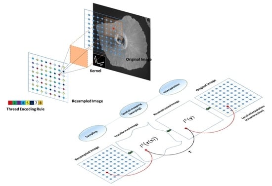
2.2.4. Secondary Image Resampling Scheme

Once the spatial transformation (warping function) is established, a resampling of the secondary image is needed to complete the registration procedure (Figure 2).
Let L and Q be the size of the rectangular reference image along the range and azimuth directions, respectively. Each pixel in the image can be associated with a discrete location x i j (with i = 1 , L ,   j = 1 , , Q ) representing a specific node of a regular grid inside the domain Ω P . Similarly, the original secondary image I S ( y m n ) is defined over a discrete regular grid { y m n :   m = 1 , M , n = 1 , , N } in the slave-image domain Ω S .
The complex-valued SAR image resampling process concerns the reconstruction of a continuous (complex) function I S ( τ ( x ) ) , from given samples of the original secondary image I S ( y m n ) , by using interpolation methods, followed by a sampling of the continuous function to a new discrete regular grid { x i j :   i = 1 , L ,   j = 1 , , Q } defined in the reference-image domain Ω P , thus determining the values I τ S ( x i j ) = I S ( τ ( x i j ) ) according to (4). It should be noted that the predictable mapped pixel positions, y = τ ( x i j ) , constitute, however, a set of irregularly-spaced data points in the domain Ω S , as pictorially illustrated in Figure 2. As a matter of fact, the image-domain coregistration procedure is employed to accommodate the topography-dependent translations of the points x defined by the non-integer field of displacement ρ ( x ) = ( ρ r ( r , a ) , ρ a ( r , a ) ) , resulting from the two different (reference and secondary) acquisition configurations.
The procedure to resample the secondary image to the regular (reference) grid is now addressed. As illustrated in the coregistration model shown in Figure 2, resampling is the process of computing the value I S ( τ ( x i j ) ) for every discrete location x i j Ω P . Conceptually, for each x i j Ω P , the algorithmic structure involves: (1) The computation of its transformed position y = τ ( x i j ) ; (2) the evaluation of the secondary image intensity I S ( y ) by interpolation, since y ( r , a )   Ω S generally falls into non-integer coordinates; and (3) the assignment of this value to the τ -warped secondary (output) image I τ S ( x i j ) .
Let us now discuss the two-dimensional (2D) interpolation procedure to reconstruct the (band-limited) continuous signal I S ( r , a ) = I S ( y ) from its discrete samples I m n S = I S ( y m n ) = I S ( r m , a n ) , associated with a regular lattice in the secondary image domain. The interpolation operation is realized via convolution of the image with a 2D interpolation kernel K ( r , a ) (Figure 3), which can be formalized as follows:
I ^ S ( r , a ) = m , n I m n S   K ( r m , a n ) .
Note that it has been implicitly assumed that the original continuous function I S is band-limited, and that the original sampling frequency is higher than the Nyquist frequency, so that the continuous function can be precisely reconstructed by its samples, at least in principle.
Separable and symmetrical interpolation kernels are commonly used to reduce the associated computational complexity. A kernel is said to be separable if K ( r , a ) = K r ( r ) K a ( a ) ; accordingly, the previous formula (10) reduces to:
I ^ S ( r , a ) = n ( m I m n S K r ( r m ) ) K a ( a n ) = n Z n ( r ) K a ( a n )   ,
where the function Z n ( r ) is defined as:
Z n ( r ) = m I m n S K r ( r m )     .
In this case, the 2D interpolation is accomplished by performing a cascade of two one-dimensional interpolations (separability): for a prescribed ( r , a ) point, the data matrix can be processed line-by-line, column-by-column. This offers more flexibility in the implementation, thus increasing the computational performance.
As sketched in Figure 3, the center of the kernel function is located at the (prescribed) center of each output sample, and then a convolution with the input signal is calculated over the filtering support (this is referred to as output-centered convolution [38]). Accordingly, this interpolation scheme requires that the kernel function has to be recalculated for each output (resampled) image pixel, which has an impact on the computation burden.
Other desirable characteristics of the kernel function are: (1) symmetry, i.e., K x ( x ) = K x ( x ) , which implies that no phase distortions are introduced since the Fourier transform of a real even function is real; and (2) partition of unity, i.e., the condition k   K x ( z k ) = 1   z , which assures the reproduction of the constant (DC filter gain).
It is evident that the tradeoff between interpolation accuracy and computational cost must be carefully considered when selecting interpolation kernels in SAR image resampling. In this investigation, we use a separable interpolation kernel; accordingly, for clarity and without loss of generality, in the following we limit our discussion to the one-dimensional case.
It is well known that the rigorous interpolation of bandlimited signals is obtained by using the ideal sin c ( x ) sin ( π x ) π x interpolation kernel. Although this kernel provides an ideal interpolation, it has a spatially infinite support, thus making its implementation impractical. A more feasible implementation is achieved by truncating the sin c function to a reasonable number of samples, thus leading to a filter with a finite support in the spatial domain, i.e., a so-called Finite Impulse Response (FIR) filter (Figure 3). However, this usually produces undesirable ringing effects in the frequency domain (Gibbs’s phenomenon), which can be mitigated by using an appropriate weighting function ψ ( x ) that gently truncates the kernel. Therefore, the interpolation is written as:
f ^ N ( x ) = k = N N f ( k Δ x ) sin c ( x k Δ x ) ψ ( x k Δ x )     ,
where we have assumed that f ( x ) is sampled at equally spaced points denoted by x k = k Δ x , Δ x being the discretization interval, and 2 N + 1 is the number of retained samples that is set as a trade-off between accuracy and computational load.
Within the SAR interferometry context, the interpolation kernel selection has been discussed in several papers [33,39,40,41,42,43]. For the truncated sin c scheme in (13), many window functions (such as Kaiser–Bessel, Blackman–Harris, cosine-like, power-law, raised-cosine, etc.) have been proposed [33]. Without loss of generality, in this paper we focus on the Knab sampling window [39] since it shows good performance in the SAR context with respect to other conventional kernels [43]. This kernel will be used for the numerical experiments discussed in the next sections. It is given in terms of a hyperbolic cosine function as follows:
ψ ( x ) = cos h ( χ 1 ( x N ) 2 ) cos h ( χ )     ,
where an adjustable factor χ = π N δ is present, and δ   ϵ   [ 0 , 1 ] is a parameter related to the oversampling factor β (i.e., the ratio between the sampling frequency and the Nyquist frequency) as follows: δ = 1 1 β . Another valid alternative is to resort to a raised-cosine kernel [44].
As a final remark, we note that the interpolation schemes discussed above are all suitable for baseband signals. However, although complex-valued SAR images are band-limited data, their spectrums are generally non-baseband in the azimuth direction, because they normally exhibit a non-zero Doppler acquisition centroid. Therefore, in order to avoid spectral distortions, the spectrum of the SAR image has to be shifted to zero Doppler (baseband) before performing the interpolation operation. Once the interpolation operation is performed, the shift along the azimuth-frequency direction should be reversed in order to restore the original center frequency of the image.

3. Parallel Scheme and Multithreading Implementation

In this Section, in order to define a parallel version of the algorithm, we first provide a brief overview of some fundamental notions of parallel computing that are relevant for our purposes [21,22,23,24] (Section 3.1); next, we present the proposed abstract parallel pattern targeted at shared-memory architectures (Section 3.2); finally, specific considerations for the practical OPENMP-based implementation in real parallel systems are addressed (Section 3.3).

3.1. Overview of Parallel Algorithm Design

The first step in designing a parallel algorithm is the problem decomposition [21]. This is the fundamental step since it has a crucial impact on the speedup and scalability that the resulting parallel implementation can achieve. In fact, it consists in defining how the computation can be effectively broken down into sub-parts that can be executed independently and concurrently. This allows identifying portions of the computation that can be assigned to different processing units and executed independently [21,22,23,24,25,26,27,28]. It is clear that the adopted problem decomposition is strictly dependent on the structure of the particular algorithm to be parallelized. Conversely, for a given problem, different decompositions and mappings may yield different performances on a given computing architecture. In the case of shared-memory architectures, mapping concerns assigning the composite tasks identified in the previous step to available threads [21,22,23,24].
After the algorithm decomposition in tasks and their assignment to the available computing resources, a key problem in obtaining optimal performances on shared-memory architectures is ensuing that the workload is well-balanced over the available processing units. The load-balancing problem consists in ensuring that all of the threads do useful work at any given time; on the contrary, an unbalanced workload implies that some threads are overloaded while others are idle (load imbalance), with a consequent detriment of the efficient use of the available computational resources [21,22,23].
Once the computational workload has been designed and decomposed in a set of concurrent tasks, the scheduling problem, which is another key issue in parallel computing, has to be addressed. The goal of scheduling is to determine an optimal assignment of tasks (corresponding to a number of threads to be created) to the processing elements available in the specific architecture and the order in which tasks should be executed.
Note that the possibility of achieving an effective load balancing is intimately connected with both the adopted task decomposition and the selected scheduling strategy. It is then clear that a key problem in obtaining optimal performance on shared-memory architectures is ensuing that the workload results are evenly balanced and that the synchronization overhead is reduced as much as possible [21,22,23].
As a final remark, it is worth emphasizing that problems in developing algorithms for shared-memory systems are often quite different from the problems encountered in distributed-memory programming. The reader is referred to the wide range of available literature for a complete discussion on parallel design [21,22,23,24,25,26,27,28,29,30].

3.2. Parallel Pattern Design of the Coregistration Algorithm

In this section, we present the general logic adopted in designing the parallel patterns for our specific SAR coregistration problem; we focus on the most relevant parts of the algorithm and provide general design guidelines, without focusing on our particular parallel algorithm implementation.
The computational problem at hand indeed involves regular structures and highly repetitive calculations, thus naturally permitting to exploit the potential degree of parallelism available in different ways and with varying degrees of coarseness. Therefore, here the objective is to design a parallel pattern structure capable of efficiently exploiting this potential parallelism, with the final goal of achieving high performance on multicore processors.
Both the warping function calculation and the resampling procedure are amenable to a convenient parallelization. In the following, we first discuss the parallel scheme of the warping function computation operation discussed in Section 2.2.3. Subsequently, we address a parallel pattern for the resampling procedure (see Section 2.2.4), which relies on a 2D convolution in the spatial image domain using a separable kernel characterized by a finite support (FIR filter), according to (11) and (12).

3.2.1. Shared-Memory Parallelism for Warping Function Computation

Parallelization of the warping function computation, which is obtained via the geometrical approach described in Section 2.2.3, requires indeed a very easy style of parallelism (nearly embarrassingly parallel scheme [21,22,23,24]). In particular, the equations in (5) have to be solved for each point of the scene, and with respect to both reference and secondary image domains; then the warp functions can be computed according to (6–8). It is important to note that the solution of (5) can be carried out independently for each point of the scene. Although the solution of (5) is iterative in nature and, therefore, in principle the associated computation time can change with the particular point of the scene under analysis, this variability is limited since the convergence is typically reached within a few iterations [9]. Moreover, the residual potential variability can be significantly mitigated by partitioning the data into different chunks that are assigned to different processing units. This arrangement is compatible with the granularity of the resulting decomposition; accordingly, we can efficiently schedule well-balanced chunks in order to achieve high performances.

3.2.2. Shared-Memory Parallelism for 2D Resampling Computation

We introduce here the parallel pattern adopted for the resampling procedure. The fact that the computation inherent to each pixel of the resampled secondary image can be carried out independently suggests a natural strategy to achieve the problem decomposition with a suitable granularity. Specifically, the adopted arrangement relies on the decomposition of the output image space domain.
Indeed, the computation of (11) for a given output pixel of the secondary image involves only the processing of a limited portion (i.e., the filter kernel support) of the input image centered on the location corresponding to the selected output pixel; this is pictorially illustrated in Figure 4. Clearly, different processing units can execute such elementary tasks simultaneously. However, the number of output pixels is generally rather larger than the number of engaged threads and, therefore, each processing unit must execute a certain number of the above-identified elementary tasks. In Figure 4, assuming eight threads are available, the thread encoding rule is schematically illustrated according to a color-coded representation: each color is associated with a distinct thread and each thread is tasked to compute the result for several output domain pixels. Accordingly, the adopted domain decomposition provides a convenient way of introducing parallelism. In fact, the amount of processing to be assigned to each elementary tasks can be determined in advance, since it depends on the image size and on the level of granularity, which is driven by the adopted problem decomposition. Such an arrangement, therefore, allows achieving, in principle, a well-balanced workload distribution across the available processing units as the number of processing units increases, thus enabling a scalable performance on shared memory architectures.
For the considered decomposition strategy, the execution time of each elementary task does not significantly depend on the considered output pixel, i.e., it exhibits a uniform distribution. Moreover, the information about tasks to be scheduled and their relations to each other is entirely known prior to the execution time. In such cases we might set up a deterministic scheduling, which shows a very limited synchronization overhead. This possibility reflects both the design options and the nature of the problem involving highly repetitive calculations. The scheduling strategy is further investigated and discussed in detail in Section 3.3.
Finally, we emphasize that the adopted parallel pattern for the coregistration of an image pair has been specifically targeted at shared-memory architectures. It is then clear that the adopted strategy is not amenable to be straightforwardly extended to distributed-memory architectures [15,22,23,24,25], due to the performance degradations associated with the arising communication overhead.

3.3. OPENMP-Based Parallel Implementation

The developed prototype used for the experimental part of this study has been implemented in the FORTRAN language, while OpenMP (Open Multi-Processing) has been used to realize the shared-memory parallelism [30].
The FORTRAN programming language is widespread in the scientific community. In fact, in the field of High Performance Computing (HPC), it has been one of the main languages used in parallel programming for a long time.
In particular, the combined use of compiled languages (e.g., C or FORTRAN) and OPENMP permits us to effectively define the parallelism in the code implementation in a highly structured way. On the contrary, dynamically interpreted languages enabling fast prototyping (e.g., Matlab, IDL, Python, etc.), which indeed are quite popular in the remote sensing community, are generally not recommended for heavy numerical computation.
This is for two main reasons: First, they generally do not allow the programmer to explicitly specify the desired parallelism scheme because of a general lack in specific support for efficient parallel computing; second, they are significantly slower in terms of execution time, thus in some cases suffering from severe performance penalties [45].
A programming paradigm targeted at shared-memory multi-processor computers is multithreaded programming [21]. OpenMP is an explicit shared-memory programming model for developing multi-threaded parallel applications, thus offering the programmer full control over parallelization; it uses the fork-join model of parallel execution [29,30] schematically illustrated in Figure 5. As a matter of fact, it has become the de facto standard for developing portable applications among a variety of shared memory architectures/platforms.
We recall that a thread is a unit of execution that can be scheduled by an operating system and that is able to independently execute a stream of instructions, and thus threads running simultaneously on multiple processors or cores might work concurrently to execute a task [21,22,23,24]. Thread handling (including synchronization), job assignments, and access coordination to shared data are implemented through OpenMP, thus allowing full specification of thread-level parallelism [30]. All threads share common memory, although they may have a number of local (private) variables. Threads working on disjoint parts can perform paralleled execution. Accordingly, the resulting implemented parallel algorithm can be executed on one or more processing units that share the available memory, by using multiple independent threads.
In our implementation, we first eliminated any real data dependency [21,22,23,24] by adapting the sequential code, and then we parallelized each processing step according to the adopted decomposition. Subsequently, the outermost loops were parallelized, according to the best practices for efficient parallel code development, thus minimizing the number of parallel regions [26,27,28,29,30]. It should be noted that there is a tradeoff between taking advantage of maximal parallelism and minimizing the synchronization overhead that contributes to the overall execution time. As a matter of fact, the implementation of thread pools that do not create and destruct threads frequently may mitigate this problem. Moreover, we highlight that the already mentioned parallelization of the outermost loops also implies a minimal overhead in thread handling and synchronization since the amount of work distributed over the different threads is maximal.
The load balancing strategy is another critical issue in parallel processing, and its implementation deserves a detailed discussion. For achieving a good load balancing, different workloads might require different scheduling strategies, according to the actual granularity of the resulting load distribution [21,22,23,24,28,30]. In particular, here we focus on two different scheduling strategies: static and dynamic scheduling.
According to the number of threads and the total number of iterations, the static scheduling strategy divides iterations into chunks, which are statically assigned to threads in the team in round-robin fashion. Although static scheduling is the least flexible strategy, it implies, however, a reduced scheduling overhead. On the contrary, in a more flexible dynamic scheduling strategy each thread executes a chunk of iterations and then requests another chunk until no chunks remain to be distributed [30].
The designed parallel pattern has been devised so that the resulting fine-grained workload distribution results are evenly distributed naturally, thus being appropriate for a static scheduling strategy. Nonetheless, to ascertain such an idea experimentally, both mentioned scheduling strategies were implemented and their experimental performance is discussed in Section 4.
Finally, it is also worth noting that we used the FFTW (Fastest Fourier Transform in the West) library, which is indeed the fastest freely available implementation of Discrete Fourier Transform (DFT) and is described in detail in [46].

4. Experimental Results and Performance Evaluation

In this Section, the implemented prototype is applied for processing real SAR data and inherent parallel performance analysis is presented and discussed, by focusing on the execution time, speedup, efficiency and scalability.

4.1. Processed SAR Data and Experimental Setup

In order to illustrate the performance of the proposed algorithm, we performed the coregistration operation on a dataset of high-resolution SAR images.
In particular, we employed a pair of Single Look Complex (SLC) SAR images acquired in the X-band by COSMO-SkyMed sensors over the volcanic Island of Fernandina in the Galapagos Archipelago (Ecuador); the main acquisition system and processing parameters are summarized in Table 1.
A multi-look version of the SAR amplitude image is shown in Figure 6a, in radar coordinates; the full resolution image size is 14,200 × 16,600 (~236 Mpixels). This dataset is particularly suitable for testing the coregistration algorithm because the imaged area is characterized by large topography variations (from sea level up to 1400 m on the top of the volcano) and the baseline of the selected pair is quite large (the perpendicular baseline is 441 m); both these characteristics imply that the warping effect is very pronounced and significantly varying all over the image. For estimation of the warping functions, we used the 0.4 arc sec Tandem-X DEM and precise orbital information. Additionally, for the 2D resampling step, we selected a rather long kernel, i.e., a 12-point Knab ( 2 N = 12), to preserve the fidelity of the resampled data. Figure 6b shows the coherence image after registration. A coherence loss on the top of the volcano is noted (see Figure 6b).
The performance analysis was carried out on two different computational platforms based on 64-bit machines (namely Platform A and Platform B).
Platform A consists of a node of an HPC cluster, equipped with two eight-core CPU Intel® Xeon E5-2660 (2.60 GHz) processors, with three levels of caches (level 1: 64 kB; level 2: 256 kB; level 3: 20 MB) each, and 384 GB of RAM. It has a storage system including an 8-TB disk and SATA (external Serial Advanced Technology Attachment) interface disk drives (in a RAID-5 configuration). HPC systems are indeed clusters consisting of several interconnected nodes. However, since this study was not concerned with the distributed performance of the algorithms, only one node at a time was used for performance evaluation.
Platform B is a laptop computer equipped with a quad-core Intel® Core™ i7-6700HQ CPU (2.60 GHz) processor with three levels of caches (level 1: 256 kB; level 2: 1 MB; level 3: 6 MB) and 16 GB of RAM. The main characteristics of the computational platforms used in this study are summarized in Table 2.
Nowadays, shared-memory architectures are designed to have a shared RAM accessed by one or more CPUs through a hierarchy of cache memories internal to each CPU. In particular, both of the employed platforms have three levels of caches (L3, L2, and L1) organized so that L3 is the largest in size but the slowest in terms of access time, while L1 is the smallest but the fastest.
Typically, the number of processing elements (cores) on a platform determines how much parallelism can be implemented. Nonetheless, many modern processors (as in the case of both platforms used in this study) also offer virtual threads. This is a technology for optimizing processor resources and hiding memory hierarchy latency; the net effect is that a single physical processor virtually appears as a set of multiple logical processors. In Intel’s terminology this is called hyper-threading, and corresponds to simultaneous multithreading (SMT) [47].

4.2. Quantitative Analysis of Speedup, Parallel Efficiency, and Scalability

In order to illustrate the benefits of parallelization, in this section we quantitatively assess the computational performance achievable by the developed multithreaded prototype in terms of canonical performance metrics. Therefore, we first introduce the basic notions of parallel speedup, efficiency and the scalability; afterwards we show the experimental results carried out on the two different shared-memory architectures introduced earlier.
The speedup factor of a parallel program is defined by the ratio [28]:
S ( N ) = T ( 1 ) T ( N )     ,
where T ( N ) is the execution time on the parallel architecture, N is the number of computing elements (processor cores) used to solve the problem, and T ( 1 ) is the execution time of the sequential implementation for the same problem. Note that the upper bound for the speedup is N , which is achieved only in ideal conditions. On the other hand, the speedup becomes unitary when the execution time of the parallel and sequential processing are the same (no improvements in the execution time). Typically, the speedup S = S ( N ) has a sub-linear trend due to inevitable parallel inefficiencies and intrinsically sequential parts [21,22]. In order to scale the speedup factor to a value between 0 and 1, the efficiency factor is usually introduced by dividing the achieved speedup by the number of allocated processing units. The efficiency is, therefore, defined as [28]:
ε ( N ) = S ( N ) N               .
Obviously, the efficiency is maximal (unitary) if S ( N ) = N , i.e., if all allocated N cores are fully exploited while executing the parallel application. Moreover, the lowest efficiency ( 1 / N ) is achieved when an application is executed sequentially using one core, while the remaining N 1 cores are allocated and do not process any task.
Preliminarily, we have experimentally verified that the implemented parallel prototype preserves the accuracy of the result attainable with the original sequential version. In addition, the experimental performance has been evaluated by averaging a sufficient number of measurements. The performances experimentally measured on platforms A and B are specifically presented and discussed in the following.
Parallel performances were evaluated in terms of speedup end efficiency, by comparing the measured execution time required for sequential and parallel implementation using various numbers of engaged threads threads/cores ( N ) . In fact, the conducted scalability analysis, with respect to the computational resources, is aimed at investigating how performance changes when the number of used processing elements increases.
We first address the experimental results obtained on platform A with the Linux operative system. Figure 7 displays the achieved performance metrics as a function of the number of engaged threads (N ∈ {1, 2, 3, 4, 8, 16, 32}), for both the static (blue) and dynamic (red) scheduling strategies. In particular, Figure 7a shows the speedup function S ( N ) , the ideal speedup being represented by the dashed line as a reference. The evaluated efficiency ε ( N ) is depicted in Figure 7b. Table 3 summarizes the numerical values of execution times and performance metrics.
As is evident in Figure 7a, the measured speedup depended on the number of threads N that were used for parallel execution. It can be seen that using more threads steadily increased the performance. Accordingly, a significant speedup and parallelization efficiency was achieved, and the speedup remained very close to the theoretical limit (see dashed line in Figure 7a), with the inherent discrepancy due to the unavoidable presence of residual sequential parts and synchronization overheads. As is well known, the speedup is limited by the inherent sequential fraction of an algorithm [21,22,23,24]. In this experiment, the sequential time was estimated to be 21s, a large part of which (16 s) is due to I/O operations. Hence, the overall estimated sequential fraction is about 6.5%. It is worth noting that by engaging 16 threads on the 16-core machines at our disposal, an efficiency of 36% giving a speedup of a factor of 5.73 was achieved, which is indeed a remarkable result on shared memory architectures. Moreover, by leveraging the hyper-threading technology it was possible to achieve a 6.81 overall speedup factor (see Table 3), with is a further significant improvement.
Finally, we stress that the sequential execution took 327 s, whereas the execution time with the multi-threaded implementation reduced to only 48 s in the case in which 32 threads were used, thus showing a remarkable reduction in runtime (see Table 3). As it is evident from Figure 7a, the achieved performance scaled to the number of the used threads. Moreover, the performances obtained with a static and dynamic scheduling strategy are quite comparable.
The considered case study (Platform A) shows that our parallel implementation reduces the execution time by a factor ranging from 6 to 7, thus making the precise (at the sub-pixel level) geometric coregistration of high-resolution SAR images practicable in a timely fashion (indicatively under one minute).
We underline again that, on this architecture, about 30–40% of the execution time of the best performance cases is spent in I/O operations; a discussion on this point is carried out later on.
The experimental results carried out on platform B using a Windows 10 professional operative system are now addressed. Figure 8 shows the achieved performance metrics as a function of the number of engaged threads N ∈ {1, 2, 3, 4, 8}, for both the static and dynamic scheduling strategies, as done for Figure 7. Table 4 summarize the numerical values of execution times and performance metrics obtained with Platform B. Specifically, the sequential time was estimated to be 10 s (of which 5 s are associated with I/O operations), hence the overall sequential fraction was 2%.
From Figure 8 we see that by engaging four threads an efficiency of about 75% was achieved with a corresponding speedup factor of about 3, for both the static and dynamic scheduling. Indeed, this is a quite remarkable result for shared memory architectures. Moreover, by leveraging the hyper-threading technology, it was possible to achieve a 4.53 overall speedup factor (see Table 4), with a relative improvement of about 30%; in this case, the dynamic scheduling performed slightly better than the static one. As for the experiments on platform A, the achieved performances scaled well with the number of engaged processing units in this case, too.
It is worth stressing that up to four threads the performances obtained with the static and dynamic scheduling strategies were quite comparable. This indicates that, according to the adopted parallel pattern, the workload distribution is evenly balanced and, therefore, a static scheduling strategy is appropriate, with no significant improvement with respect to the more flexible dynamic scheduling. Conversely, as is evident from Figure 8 (see shaded areas), the adoption of dynamic scheduling might be advantageous, when hyper-threading is used.
It is worth emphasizing that the pertinent inefficiencies are mainly ascribable to the (residual) sequential parts of the algorithm as well as to the unavoidable synchronization overheads.
In this second case study (Platform B), the obtained execution time reduction was also considerable, thus making the precise coregistration achievable very quickly even on a low-cost laptop (indicatively about 100 s).
A discussion regarding the different performances is now in order. To this end, we need to analyze the differences in the hardware characteristics of the two architectures.
Platform A has an overall better performing cache compared to platform B because of the larger L3 cache (20 MB vs. 6 MB); this implies that more data can be stored in the L3 cache for access by each of the CPUs. Platform A also has a relatively larger memory bandwidth (51.2 GB/s vs. 34.1 GB/s), which is the maximum rate at which data can be read from or stored into memory. As a matter of fact, memory-intensive threaded applications can suffer from memory bandwidth saturation as more threads are introduced [30]. In addition, platform A has more processing physical cores (16 vs. 4) resulting in a wide available parallelism. Conversely, platform B has a higher turbo clock speed (3.5 GHz vs. 3 GHz), which can boost to a higher clock speed in order to offer increased performance, and a higher RAM speed (2133 MHz vs. 1600 MHz).
A crucial factor limiting the parallel performance obtained on platform A with respect to platform B can be attributed to their different storage systems. In fact, platform A is equipped with a set of hard disk drives (electro-mechanical) in a RAID-5 (Redundant Array of Independent/Inexpensive Disks) configuration, while platform B has a solid-state drive (SSD). It is well known that SSDs are substantially faster and more responsive than electro-mechanical hard disk drives; moreover, a further loss of performance is due the use of a redundant file system (RAID-5 configuration) that is designed and optimized for increasing the robustness to hardware faults and not the data access speed. For these reasons, as the inputs are loaded into the RAM before processing, or the coregistered image is finally saved on the storage system, the relatively reduced I/O speed of platform A turns out in an equivalent augmented sequential part of the workload, with consequent detriment of the overall parallel efficiency in accordance with Amdahl’s law [24,28].
It is important to remark that the designed parallel algorithm largely relies on in-memory data management and processing. Accordingly, it works mainly on data stored in the RAM, thus reducing a large part of the slow data accesses (I/O). Nonetheless, some I/O operations involving the large images to be processed (e.g., at the beginning and at the end of processing) remain unavoidable.
The abovementioned differences in the storage systems mostly explain the relatively slightly better performance in terms of scalability achieved on platform B with respect to that of platform A. According to our results, a primary challenge in large-data processing is to overcome the I/O bottleneck, and thus the use of SSDs may be suggested where performance is critical.
As a final remark, we underline that the experiments carried out on both platforms demonstrate that the developed parallel prototype is easily portable and effectively applicable, with scalable performance, to available multiprocessor platforms, which might have different operative systems and architectures, and a variable number of processing cores.

5. Conclusions

In this paper, a parallel approach to the SAR image coregistration problem was explored with the objective of taking advantage of the parallelism offered by currently and widely available shared-memory multicore architectures. Specifically, we have proposed a rigorous and efficient parallel algorithm based on multithreading by relying on high-performance computing (HPC) methods [21,22,23,24,25,26,27,28,29,30] and with no accuracy loss.
Methodologically, the algorithm was preliminarily framed mathematically. Subsequently, a parallel version was proposed by suitably designing its parallel pattern and implementing the parallelism at the thread level. OpenMP and the modern Fortran programming language were employed to develop a highly efficient and portable multithread prototype processing code.
The parallel performance of the implemented prototype processor was experimentally investigated and quantitatively assessed by processing real high resolution SAR data and using two different multicore architectures. The experimental analysis was conducted by evaluating suitable performance metrics, which demonstrated the effectiveness of the adopted parallel strategy. The scalable performance of the proposed solution has also been investigated.
The implemented thread-level parallelism exhibited significant speedup and scalable performances, thus enabling the full exploitation of the ubiquitous availability of shared memory computing platforms, such as general-purpose multicore CPUs. Moreover, the parallel prototype offers a high degree of portability on different operating systems (e.g., Windows and Linux) as well.
As a result, the developed high performance prototype enables large scale and fast SAR image coregistration operation on shared-memory multiprocessor systems; for this reason, it can be advantageously and systematically applied in the interferometric processing of multi-pass SAR datasets.
The implemented parallel pattern may be easily extended to different SAR configurations, and future developments will be specifically devoted to the application of the implemented prototype solution to data of other SAR sensors (e.g., Sentinel-1) and multimode configurations [48].

Author Contributions

P.I. and E.S. conceived the work; P.I. set up the parallel procedures, implemented the software prototype and carried out the experiments; P.I. prepared the original draft of the manuscript; P.I. and E.S. reviewed and edited the manuscript. All authors have read and agreed to the published version of the manuscript.

Funding

This research received no external funding.

Acknowledgments

The authors wish to thank Diego Reale and Antonio Pauciullo for their help in setting up the experimental part of this work and for valuable suggestions and discussions. The authors also acknowledge the technical support provided by Simone Guarino. COSMO-SkyMed data have been provided by Italian Space Agency through the CEOS Volcano Demonstrator (https://ceos.org/ourwork/workinggroups/disasters/volcanoes/ (accessed on 4 April 2021)). The DEM used in this investigation has been also obtained through the CEOS Volcano Demonstrator.

Conflicts of Interest

The authors declare no conflict of interest.

References

  1. Le Moigne, J.; Netanyahu, N.S.; Eastman, R.D. (Eds.) Image Registration for Remote Sensing; Cambridge University Press: Cambridge, UK, 2011. [Google Scholar]
  2. Fornaro, G.; Franceschetti, G.; Lanari, R.; Sansosti, E.; Tesauro, M. Global and local phase-unwrapping techniques: A comparison. J. Opt. Soc. Am. A 1997, 14, 2702–2708. [Google Scholar] [CrossRef]
  3. Fornaro, G.; Sansosti, E. A two-dimensional region growing least squares phase unwrapping algorithm for interferometric SAR processing. IEEE Trans. Geosci. Remote Sens. 1999, 37, 2215–2226. [Google Scholar] [CrossRef]
  4. Imperatore, P.; Pepe, A.; Lanari, R. Multichannel Phase Unwrapping: Problem Topology and Dual-Level Parallel Computational Model. IEEE Trans. Geosci. Remote Sens. 2015, 53, 5774–5793. [Google Scholar] [CrossRef]
  5. Tian, Q.; Huhns, M.N. Algorithms for subpixel registration. Comput. Vis. Graph. Image Process. 1986, 35, 220–223. [Google Scholar] [CrossRef]
  6. Brown, L.G. A survey of image registration techniques. ACM Comput. Surv. 1992, 24, 325–376. [Google Scholar] [CrossRef]
  7. Scheiber, R.; Moreira, A. Coregistration of interferometric SAR images using spectral diversity. IEEE Trans. Geosci. Remote Sens. 2000, 38, 2179–2191. [Google Scholar] [CrossRef]
  8. Liao, M.; Lin, H.; Zhang, Z. Automatic registration of InSAR data based on least-square matching and multi-step strategy. Photogramm. Eng. Remote Sens. 2004, 70, 1139–1144. [Google Scholar] [CrossRef]
  9. Sansosti, E.; Berardino, P.; Manunta, M.; Serafino, F.; Fornaro, G. Geometrical SAR image registration. IEEE Trans. Geosci. Remote Sens. 2006, 44, 2861–2870. [Google Scholar] [CrossRef]
  10. Guizar-Sicairos, M.; Thurman, S.T.; Fienup, J.R. Efficient subpixel image registration algorithms. Opt. Lett. 2008, 33, 156–158. [Google Scholar] [CrossRef] [PubMed] [Green Version]
  11. Li, Z.; Bethel, J. Image coregistration in SAR interferometry. Proc. Int. Arch. Photogramm. Remote Sens. Spatial Inf. Sci. 2008, 37, 433–438. [Google Scholar]
  12. Liu, B.Q.; Feng, D.Z.; Shui, P.L.; Wu, N. Analytic search method for interferometric SAR image registration. IEEE Geosci. Remote Sens. Lett. 2008, 8, 294–298. [Google Scholar]
  13. Nitti, D.O.; Hanssen, R.F.; Refice, A.; Bovenga, F.; Nutricato, R. Impact of DEM Assisted Coregistration on High-Resolution SAR Interferometry. IEEE Trans. Geosci. Remote Sens. 2011, 49, 1127–1143. [Google Scholar] [CrossRef]
  14. Solaro, G.; Imperatore, P.; Pepe, A. Satellite SAR Interferometry for Earth’s Crust Deformation Monitoring and Geological Phenomena Analysis. In Geospatial Technology—Environmental and Social Applications; InTech: Rijeka, Croatia, 2016. [Google Scholar]
  15. Franceschetti, G.; Imperatore, P.; Iodice, A.; Riccio, D. Radio-coverage parallel computation on multi-processor platforms. In Proceedings of the 2009 European Microwave Conference (EuMC), Rome, Italy, 29 September–1 October 2009; pp. 1575–1578. [Google Scholar]
  16. Imperatore, P.; Pepe, A.; Lanari, R. High-performance parallel computation of the multichannel phase unwrapping problem. In Proceedings of the 2015 IEEE International Geoscience and Remote Sensing Symposium (IGARSS), Milan, Italy, 26–31 July 2015; pp. 4097–4100. [Google Scholar]
  17. Imperatore, P.; Pepe, A.; Berardino, P.; Lanari, R. A segmented block processing approach to focus synthetic aperture radar data on multicore processors. In Proceedings of the 2015 IEEE International Geoscience and Remote Sensing Symposium (IGARSS), Milan, Italy, 26–31 July 2015; pp. 2421–2424. [Google Scholar]
  18. Imperatore, P.; Pepe, A.; Lanari, R. Spaceborne Synthetic Aperture Radar Data Focusing on Multicore-Based Architectures. IEEE Trans. Geosci. Remote Sens. 2016, 54, 4712–4731. [Google Scholar] [CrossRef]
  19. Imperatore, P.; Zinno, I.; Elefante, S.; de Luca, C.; Manunta, M.; Casu, F. Scalable performance analysis of the parallel SBAS-DInSAR algorithm. In Proceedings of the 2014 IEEE Geoscience and Remote Sensing Symposium, Quebec City, QC, Canada, 13–18 July 2014; pp. 350–353. [Google Scholar]
  20. Plaza, A.; Du, Q.; Chang, Y.L.; King, R.L. Special Issue on High Performance Computing in Earth Observation and Remote Sensing. IEEE J. Sel. Top. Appl. Earth Obs. Remote Sens. 2011, 4, 503–507. [Google Scholar] [CrossRef] [Green Version]
  21. Foster, I. Designing and Building Parallel Programs: Concepts and Tools for Parallel Software Engineering; Addison-Wesley: Reading, MA, USA, 1995. [Google Scholar]
  22. Dongarra, J.; Foster, I.; Fox, G.; Gropp, W.; Kennedy, K.; Torczon, L.; White, A. Sourcebook of Parallel Computing; Morgan Kaufman Publishers: San Francisco, CA, USA, 2003. [Google Scholar]
  23. Mattson, T.G.; Sanders, B.; Massingill, B. Patterns for Parallel Programming; Addison-Wesley: Boston, MA, USA, 2005. [Google Scholar]
  24. Pacheco, P.S. An Introduction to Parallel Programming; Morgan Kaufmann: Burlington, MA, USA, 2011. [Google Scholar]
  25. Gropp, W.; Gropp, W.D.; Lusk, E.; Skjellum, A.; Lusk, A.D.F.E.E. Using MPI: Portable Parallel Programming with the Message-Passing Interface; MIT Press: Cambridge, MA, USA, 1999. [Google Scholar]
  26. Akl, S.G. The Design and Analysis of Parallel Algorithms; Prentice Hall: Englewood Cliffs, NJ, USA, 1989. [Google Scholar]
  27. Hager, G.; Wellein, G. Introduction to High Performance Computing for Scientists and Engineers; CRC Press: Boca Raton, FL, USA, 2010. [Google Scholar]
  28. El-Rewini, H.; Abd-El-Barr, M. Advanced Computer Architecture and Parallel Processing; John Wiley & Sons, Inc.: Hoboken, NJ, USA, 2005. [Google Scholar]
  29. Gebali, F. Algorithms and Parallel Computing; John Wiley & Sons, Inc.: Hoboken, NJ, USA, 2011. [Google Scholar]
  30. Chapman, B.; Jost, G.; van der, R.P. Using OpenMP: Portable Shared Memory Parallel Programming; MIT Press: Cambridge, MA, USA, 2007. [Google Scholar]
  31. Knapp, C.H.; Carter, G.C. The generalized correlation method for estimation of time delay. IEEE Trans. Acoust. Speech Signal Process. 1976, 24, 320–327. [Google Scholar] [CrossRef] [Green Version]
  32. Glasbey, C.A.; Mardia, K.V. A review of image-warping methods. J. Appl. Stat. 1998, 25, 155–171. [Google Scholar] [CrossRef] [Green Version]
  33. Wolberg, G. Digital Image Warping; IEEE Computer Society Press: Los Alamitos, CA, USA, 1990; Volume 10662. [Google Scholar]
  34. Foroosh, H.; Zerubia, J.B.; Berthod, M. Extension of phase correlation to subpixel registration. IEEE Trans. Image Process. 2002, 11, 188–199. [Google Scholar] [CrossRef] [Green Version]
  35. Sansosti, E. A Simple and Exact Solution for the Interferometric and Stereo SAR Geolocation Problem. IEEE Trans.Geosci. Remote Sens. 2004, 42, 1625–1634. [Google Scholar] [CrossRef]
  36. Fornaro, G.; Sansosti, E.; Lanari, R.; Tesauro, M. Role of processing geometry in SAR raw data focusing. IEEE Trans. Aerosp. Electron. Syst. 2002, 38, 441–454. [Google Scholar] [CrossRef]
  37. Pepe, A.; Berardino, P.; Bonano, M.; Euillades, L.D.; Lanari, R.; Sansosti, E. SBAS-Based Satellite Orbit Correction for the Generation of DInSAR Time-Series: Application to RADARSAT-1 Data. IEEE Trans. Geosci. Remote Sens. 2011, 49, 5150–5165. [Google Scholar] [CrossRef]
  38. Goodman, W.G.; Carrara, R.S.; Majewski, R.M. Spotlight Synthetic Aperture Radar Signal Processing Algorithms; Artech House: Boston, USA, 1995; pp. 245–285. [Google Scholar]
  39. Knab, J.J. Interpolation of band-limited functions using the approximate prolate series. IEEE Trans. Inf. Theory 1979, IT-25, 717–720. [Google Scholar] [CrossRef]
  40. Knab, J.J. The sampling window. IEEE Trans. Inf. Theory 1983, IT–29, 157–159. [Google Scholar] [CrossRef]
  41. Keys, R. Cubic convolution interpolation for digital image processing. IEEE Trans. Acoust. Speech Signal Process. 1981, 29, 1153–1160. [Google Scholar] [CrossRef] [Green Version]
  42. Hanssen, R.; Bamler, R. Evaluation of interpolation kernels for SAR interferometry. IEEE Trans. Geosci. Remote Sens. 1999, 37, 318–321. [Google Scholar] [CrossRef]
  43. Migliaccio, M.; Bruno, F. A new interpolation kernel for SAR interferometric registration. IEEE Trans. Geosci. Remote Sens. 2003, 41, 1105–1110. [Google Scholar] [CrossRef]
  44. Cho, B.L.; Kong, Y.K.; Kim, Y.S. Interpolation using optimum Nyquist filter for SAR interferometry. J. Electromagn. Waves Appl. 2005, 19, 129–135. [Google Scholar] [CrossRef]
  45. Gmys, J.; Carneiro, T.; Melab, N.; Talbi, E.G.; Tuyttens, D. A comparative study of high-productivity high-performance programming languages for parallel metaheuristics. Swarm Evol. Comput. 2020, 57, 100720. [Google Scholar] [CrossRef]
  46. Frigo, M.; Johnson, S.G. The design and implementation of FFTW3. Proc. IEEE 2005, 93, 216–231. [Google Scholar] [CrossRef] [Green Version]
  47. Rauber, T.; Rünger, G. Parallel Programming, for Multicore and Cluster Systems; Springer: Berlin/Heidelberg, Germany, 2010. [Google Scholar]
  48. Pepe, A.; Impagnatiello, F.; Imperatore, P.; Lanari, R. Hybrid Stripmap–ScanSAR Interferometry: Extension to the X-Band COSMO-SkyMed Data. IEEE Geosci. Remote Sens. Lett. 2018, 15, 330–334. [Google Scholar] [CrossRef]
Figure 1. SAR SLC Image Coregistration Functional Scheme.
Remotesensing 13 01963 g001
Figure 2. Conceptual scheme of finely co-registered secondary image reconstruction.
Remotesensing 13 01963 g002
Figure 3. Pictorial description of the convolution-based 2D interpolation scheme based on a finite-support kernel in the spatial domain.
Remotesensing 13 01963 g003
Figure 4. Parallel scheme of the reconstruction operation based on the convolution of the 2D image with a 2D interpolation kernel: different colors are associated with distinct threads in the pictorial representation.
Remotesensing 13 01963 g004
Figure 5. A sketch of the fork-join model.
Remotesensing 13 01963 g005
Figure 6. (a) Multilook COSMO-SkyMed image acquired (on 27 April 2018) over Fernandina Island (Galapagos) obtained after coregistration on the reference image (acquired on 11 April 2018); (b) coherence between secondary and reference SAR images evaluated after the image coregistration operation.
Remotesensing 13 01963 g006
Figure 7. Experimental performance measured on platform A as a function of the number of engaged threads/cores ( N ) , for both static (blue) and dynamic (red) scheduling strategies: (a) Speedup factor S ( N ) (continuous lines) and ideal speedup (dashed line) shown as a reference; (b) efficiency ε ( N ) . Shaded areas in the graphs corresponds to the number of additional threads provided by the hyper-threading technology.
Remotesensing 13 01963 g007
Figure 8. Same as Figure 7, but for platform B.
Remotesensing 13 01963 g008
Table 1. Parameters of the SAR dataset.
ParameterReferenceSecondary
Acquisition Date11-APR-201827-APR-2018
Orbit Directiondescending
Image Size (range × azimuth)16,600 × 14,200
Real Azimuth Antenna Dimension [m]5.6
Carrier Frequency [GHz]9.60
Range Sampling Frequency [MHz]84.38
Pulse Repetition Frequency—PRF [Hz]3114.62
Range Bandwidth [MHz]69.73
Processed Range Bandwidth100%
Azimuth Bandwidth [kHz]2.60
Processed Azimuth Bandwidth100%
Mean Doppler centroid [kHz]−417.19 −553.26
Azimuth Pixel Spacing [m]2.33
Range Pixel Spacing [m]1.78
Perpendicular Baseline [m]441
Parallel Baseline [m]625
Table 2. Utilized parallel architectures.
PlatformCPUNumber of
Processors
RAM Physical MemoryNumber of
Physical Cores
Number of
Logical Cores (1)
AIntel® Xeon CPU
E5-2660 @ 2.20 GHz
2384 GB1632
BIntel® Core™
i7-6700HQ CPU @2.60 GHz
116 GB48
1 Hyperthreading.
Table 3. Averaged parallel performance achieved on the two eight-core Intel® Xeon CPU E5-2660 (2.20 GHz) CPU architecture (Platform A) for a 16,600 × 14,200 image size.
Number of Engaged Threads12481632 (1)Scheduling
Speedup11.602.764.405.716.20Static
Efficiency10.780.600.450.350.19
Execution time (s)327204118745752
Speedup11.602.774.415.736.81Dynamic
Efficiency10.800.690.550.360.21
Execution time (s)327204118745748
Estimated sequential time (s)21
1 16 physical cores, 32 logical units.
Table 4. Averaged parallel performance achieved on Intel® Core™ i7-6700HQ CPU (2.60 GHz) architecture (Platform B) for a 16,600 × 14,200 image size.
Number of Engaged Threads1248 (1)Scheduling
Speedup11.822.954.04Static
Efficiency 10.910.740.50
Execution time (s) 517284175128
Speedup11.853.014.53Dynamic
Efficiency 10.920.750.57
Execution time (s) 517280172114
Estimated sequential time (s)10
1 four physical cores, eight logical units.
Publisher’s Note: MDPI stays neutral with regard to jurisdictional claims in published maps and institutional affiliations.

