1. Introduction
Thanks to their ability to collect measurements on both the horizontal (H) and vertical (V) polarization of the transmitted/received electromagnetic signal, dual-polarization weather radars play a central role in both operational and research environments. While the largest systems constitute the backbone of the remote sensing capabilities of many meteorological services, like the Swiss Federal Office of Meteorology and Climatology (MeteoSwiss) [
1], their smaller and mobile counterparts aid us in the understanding of precipitation in the most remote locations, such as the Antarctic continent [
2].
Among the polarimetric variables, differential reflectivity plays a special role for its direct link with the axis ratio of the observed hydrometeors. Phenomena like aggregation and riming affect size and shape of ice particles, influencing
in turn [
3,
4,
5]. Consequently, the scrutiny of values and variations of the differential reflectivity can help identify the occurrence of these microphysical processes [
6,
7].
In a realistic scenario, various factors can affect the two channels and this can result in an artificial offset in this variable, which can cause the misinterpretation of the meteorological signals. A typical example is the effect on automated hydrometeor classifications, such as the semisupervised one included in the Python ARM Radar Toolkit [
8,
9], where a sufficiently large bias in
can shift the output from a hydrometeor class to another. Therefore, a calibration technique is required to identify this offset and subtract it from the measurements before they can be used in any scientific or operational application.
The commonly accepted level of accuracy in
for diverse hydrometeorological applications varies between 0.1 and 0.2 dB [
10]. Over the years, several calibration methods have been proposed by the scientific community and the topic is an active research area. One of the first ones to be developed was the “birdbath” technique [
11]. This technique estimates the
bias from measurements collected in light rain during Plan Position Indicator (PPI) scans performed at 90
elevation. It is considered an accurate reference point, and it is often used for comparison purposes in more recent studies [
12]. However, liquid precipitation is often absent in datasets collected in mountainous or polar regions and this limits the applicability of the method.
An interesting alternative that does not suffer from the same limitation is the technique proposed by [
13], which relies on dry snow observations in Range Height Indicator (RHI) scans. It depends on the output of an automated hydrometeor classification for the identification of suitable regions in the scan. This constitutes an obstacle, when the classification algorithm, such as [
8,
14], requires an already calibrated
field in input. Similar usage of RHI scans can be seen in the work of [
15], where the
bias is derived from observations at different elevations angles of rain. As for the “birdbath” technique, its usage is constrained by the presence of a sufficient amount of measurements collected in liquid precipitation.
A completely different approach has been proposed by [
12,
16], which relies on the cross-polar power measurements for determining the calibration offset. Dual-polarization systems can be classified into polarization-diverse or polarization-agile, depending on whether the transmission of the H and V channels is simultaneous or alternate. While the method can be applied to radars belonging to the second category, the polarization-diverse ones are incapable of recording the required cross-polar power measurement. Another distinct technique is engineering calibration [
17]. It requires accurate monitoring of the transmitting and receiving chain of the radar hardware, which is not always performed before or during field campaigns. Similarly, a calibration based on hybrid measurements, currently used for the WSR-88D radar network, can be found in [
18] (p. 151). The same network takes advantage of the known properties of Bragg scattering of targets such as light rain, aggregates or clear air, as highlighted in [
19,
20].
In this study we propose a calibration method that takes inspiration from the “birdbath” technique, while overcoming its dependence on measurements in rain, and that addresses the recurrent question of how the
bias correction should evolve in time. To estimate its temporal dependence, we follow a different approach from previous studies [
12,
13], using solely the polarimetric variables provided by the radar. The proposed method has been designed to be generally usable by the radar community, with the caveat of having to fine-tune some of the thresholds in the algorithm, and it has been successfully tested on two different radars.
The first key aspect addressed by the method is the automated selection of a section of the vertical profiles suitable for the calibration. The choice is based on the analysis of the empirical probability density function of the measurements at each range gates. The deployment in mountainous or polar regions, the presence of excessive clutter, or technical issues affecting the lowest range gates, are all factors that may limit or completely deny access to measurements in liquid precipitation. Therefore, our algorithm does not limit the choice of this suitable vertical section to the sole rain or snow region of the profiles.
A topic directly linked to this first phase is whether radar volumes dominated by snow or ice are suitable for calibration purposes. Even though the formers have been mentioned as viable targets in other scientific studies [
21], quantitative estimation of the agreement between measurements from the two mediums are scarce in the scientific literature. Examples can be found in [
22,
23], in which comparisons of the time series of bias estimates from light rain and from dry snow are presented. To complement those studies and to further confirm the validity of our method we carried out a simple test, comparing solid hydrometeors with light rain from the same vertical PPI scans.
The second key aspect is the handling of the eventual temporal evolution of the
offset, since its variability is a common point on which some recent methods agree upon [
12,
21]. The PPI scans, available at regular intervals, are utilized as a starting point to compensate for these fluctuations. While each of them provides us with a single calibration value at an exact date and time, the real challenge lies in determining the bias between these point values. The proposed approach, based on an ordinary kriging interpolation [
24] (p. 119), defines a function able to compute the
offset at any time in the campaign, by taking into account the typical timescale on which the fluctuations take place. Incidentally, this solution gives us an estimate of the uncertainty on calibration, whose value grows with the distance from the interpolated points.
The study is structured as follows.
Section 2 provides a list of the datasets used in the study, accompanied by a description of the polarimetric variables available in each of them.
Section 3 illustrates the method, explaining in detail the two main steps in which it is divided, and investigating the adequateness of radar volumes dominated by solid hydrometeors for the purpose of calibration. In
Section 4 the results for all campaign are displayed, including a comparison of the calibrated
fields of the two radars available during one campaign. Finally,
Section 5 provides the summary and the conclusions of the study.
2. Data
A key role is played in this study by an X-band, dual-polarization, Doppler, scanning weather radar (MXPol), with a magnetron (model M1458A produced by New Japan Radio Co., Ltd. Microwave Division) at the core of its Transmit–Receive (TR) chain. Precipitation measurements collected by this radar during five field campaigns, listed in
Table 1, have been used for defining and testing the proposed calibration algorithm.
Each dataset comprises a series of PPI scans at 90 elevation, performed approximately every 5 min. For every campaign, we will denote the date and time of each scan with , where i is a discrete index that can assume any integer value between 1 and a total , dependent on the duration of the deployment of the radar on the field. The 360 rotation of the antenna dish during the PPI is discretized into some azimuth angles, each denoted by , with . For each of these angles, data are recorded at certain range gates , with k varying between 1 and the number of range gates . The quantities , and are all campaign-dependent.
The variables taken in consideration for this study, available for all campaigns and at each coordinate triplet , are:
Reflectivity factor for horizontal polarization, [dBZ],
Differential reflectivity, [dB],
Co-polar correlation coefficient, [-],
Signal to noise ratio, on the horizontal ( [dB]) and vertical ( [dB]) channels.
During the PAYERNE campaign, we have access to a second dataset of vertical PPI scans performed by another X-band, dual-polarization, Doppler, scanning weather radar (DX50), belonging to MeteoSwiss and deployed by their personnel at a distance of approximately 3.7 km from MXPol. This data series is slightly shorter, encompassing only the period between 1st and 23rd May 2014, while the frequency of the scans is doubled. Another difference between the two datasets is in the recorded variables: and are unavailable for DX50, and for the remaining fields we do not know the measurements at each of the azimuth angles in which the rotation has been divided. Instead, an averaged value at each range gate was recorded.
In addition to the PPI scans, a series of RHI scans is available for each radar. Due to the choice of azimuth angle, they lie on the same plane and several overlapping volumes can be identified for each couple of scans. The list of variables for these RHI scans is the same as the PPI case, although measurements are available at different elevations (, with ), instead of azimuth angles, due to the geometry of the scans.
Even though all the datasets mentioned above are used as input for the proposed calibration method, all the steps leading from the original scans to the final bias computation will be illustrated only for PAYERNE. This choice is motivated by the need for succinctness in illustrating the procedure, and by the convenience of using the same campaign for the evaluation section, in which the calibrated RHI scans of MXPol and DX50 will be compared.
All the data used for the study have been uploaded at [
25].
3. Calibration Method
The proposed calibration method, inspired by the “birdbath” technique [
11], uses measurements collected from PPI scans at 90
elevation, in both liquid and solid precipitation, to define a time-varying bias. For each campaign, any scan can be calibrated by subtracting this bias, computed at the correct date and time, from the
field.
The classical “birdbath” method relies on the approximately circular cross-section of raindrops, in light precipitation events, when observed at the zenith from the ground, which results in a measured
dB. The average over a full 360
rotation in azimuth removes deviations from this theoretical value due to a non-zero canting angle of raindrops [
11]. Our method also includes measurements collected in solid precipitation, so we cannot assume the same circular cross-section for the observed hydrometeors. We hypothesize that full azimuthal rotations are enough to compensate the uneven shapes of ice and snow in a sufficiently homogeneous radar volume, and therefore the theoretical center of the distribution of
values recorded at evenly spaced angles across multiple vertical PPI scan is approximately equal to 0 dB. This hypothesis will be tested in
Section 3.2.
In the following, a technique for automatically identifying the radar volumes suitable for the computation of the bias is first presented, and the evolution in time of this bias is then defined.
3.1. Filtering the “Birdbath” PPI Scans
3.1.1. Outline
The first half of the calibration process started from the complete PPI scans collected during an entire campaign (here PAYERNE for illustration), from which a subset of measurements that would be used for the final bias computation was extracted. The procedure started by imposing thresholds directly on the polarimetric variables, to exclude measurements unsuitable for calibration purposes. This step is described in details in
Section 3.1.2.
The second part, described in
Section 3.1.3, describes how the remaining measurements were distributed at each of the range gates. The aim of this subsection was the removal of all the unrealistically high or low
values recorded in the lowest range gates in MXPol scans, as visible in
Figure 1, panel (
a).
These extreme measurements were caused, in our case, by the aging of the TR limiter, a component of the radar in charge of blocking the transmitted pulse, but not the received one, from passing through the receiver [
26] (p. 31). It should be noted that the filtering addressed the presence of a significant drift in
independently from its cause.
The third and final step enforced the presence of a minimum number of measurements at each time step and in longer time interval. The output of this analysis, described in
Section 3.1.4, represented the input of the second half of the calibration process, described in
Section 3.3.
3.1.2. Thresholds on Polarimetric Variables
The procedure described in this section aimed to remove noisy data to enforce a condition of sufficient homogeneity within the radar volumes used for the analysis, by setting some thresholds on few polarimetric variables. Additionally, the filtering removed the measurements collected in the ”bright band” related to the melting layer, where we usually observe a shift of the distribution towards higher values. The variable and conditions chosen were:
dB and dB, to select measurement deriving from a clear return signal;
, to limit the analysis to the more homogeneous among the radar volumes, in terms of size, shape and density of particles;
, a condition on a derived variable chosen as proxy for the bright band location, loosely based on [
27], to exclude data too close to the melting layer height. The quantities
and
are respectively the normalized and dimensionless reflectivity factor for horizontal polarization ([0,60] dBZ → [0,1]) and co-polar correlation coefficient ([0.65, 1.0] → [0, 1]).
If a measurement was excluded, all the data at the same range gate in that specific PPI scan were removed, too. In this way, we ensured that all the azimuth angles in which the 360 was discretized were equally represented in the resulting dataset.
The thresholds were manually defined, monitoring their effect on the empirical distribution and the total number of the remaining measurements, for all the campaigns. While the chosen values appeared to be adequate for the two X-band radars used in the analysis, we could not exclude the possibility that other radar systems, especially the ones operating at different frequencies, may have needed a re-tuning of these parameters. In general, excessively permissive conditions have the undesired result of allowing more extreme values in the distribution. On the other hand, restrictive ones overly reduce the total number of values. For the PAYERNE campaign, varying the threshold on between 0.85 and 0.95 resulted in small changes (order of 0.1 dB) in the quantile 0.95 of the empirical distribution. However, larger changes could be seen for the quantile 0.99, where moving the minimum accepted from 0.85 to 0.95 halved the value of the quantile, reducing the tail of the distribution. This also resulted in a loss of around measurements, lowering the remaining total number to around . The effect of halving or doubling the threshold on was much lower lower, and barely noticeable when the condition was imposed. Another reasoning led us to the choice of conditions on : since the field campaigns considered in the analysis had a different minimum value for this variable, we decided to even the analysis by choosing the highest minimum value, equal to 5 dB.
3.1.3. Selection of Suitable Range Gates
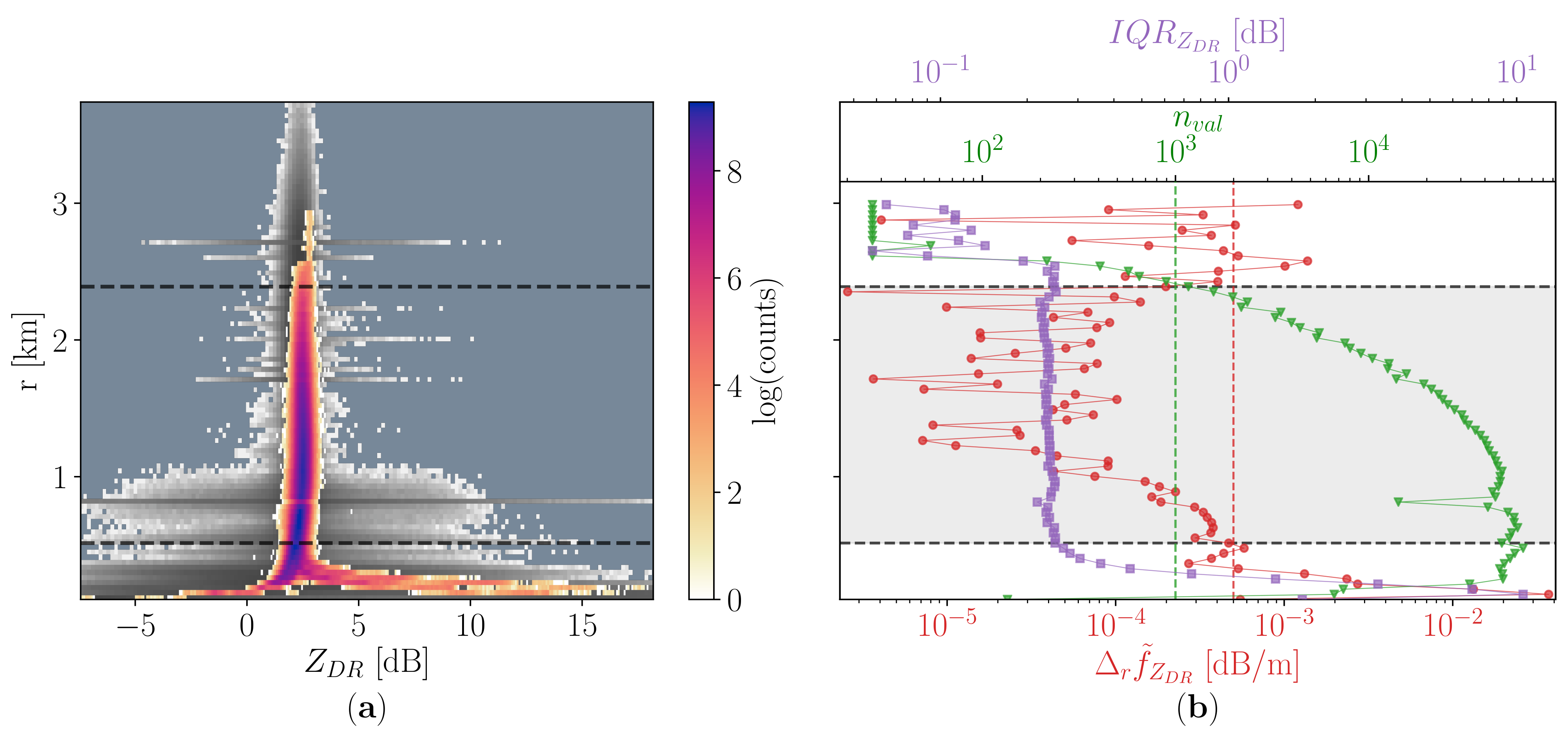
The second step involved the study of the empirical probability density function of the remaining differential reflectivity values at each range gate, , computed using data from all the events of the campaign. The random variable u spanned the sample space given by all combinations of and with valid measurements at the range . The goal was to select the range gates without the extreme values mentioned at the beginning of this section. Therefore, we needed to isolate the almost uniform region in the upper part of the profile, by thresholding quantities that varied significantly closer to the radar, where the issue lay.
We started by counting the number of valid measurements at each range gate,
. After computing the median of every distribution,
, we also estimated the absolute value of its variation in range defining the quantity:
The purpose of this new variable was to detect when the center of the various in the profile bent toward the extremely high or low values observed in the lower range gates. We opted for the usage of the median instead of the mean value to identify the aforementioned centers since the former was less affected by the presence of outliers, which could cause spurious shifts in the center values and in turn introduce noise in the estimate of their variation in range.
On the two newly defined quantities we imposed the conditions:
, to ensure the significance of the statistics used;
dB m, to ensure limited variability in the profile.
Once again, the effect of these thresholds on the total number of the remaining measurements were monitored when we manually selected their value. In addition, we took into account the number of range gates accepted into the selected region of the profiles and the impact on the median value of the empirical distribution at each of them. In the PAYERNE case, varying the minimum threshold on between 500 and 2000 had a smaller effect on all the monitored parameters than moving the one on between dB m and dB m. In both cases, the effect on the lower quantiles was more marked than on the upper ones. While the maximum of the distribution changed by less than 0.1 dB, the range of possible values for the minimum one spanned approximately 0.4 dB. The chosen thresholds on gives us a minimum of about 2.2 dB, roughly 0.2 dB higher than what would be obtained using the most permissive condition among the tested ones. A value lower than 0.0005 dB m, however, resulted in a sharp drop of both the total number of measurements and of accepted range gates. Since the limit on was chosen to ensure the significance of all range gates included in the analysis, its effect on the monitored statistics was less evident. While an increase of had only a limited impact on the number of selected gates, definitely smaller than the one of observed for , its decrease to 500 or 750 changed the maximum of the distribution by slightly less than 0.5 dB.
In some cases, such as the DAVOS campaign, this drift of the approximate center was accompanied by a broadening of the distributions. However, this was not a behavior that we could simply capture by the sole thresholding of their interquartile range,
. Instead, we wanted to capture how
increased with respect to the campaign-dependent typical value of the upper part of the profile, where the distributions are narrower. Thus we computed the median of the interquartile ranges in the top half of the valid range gates, and we set a threshold equal to 0.2 dB on the absolute difference between
and this median value. This last threshold had no effect on the PAYERNE dataset, since the
profile was particularly constant, as can be seen in
Figure 1, panel (
b), where
,
and
are plotted together with their relative thresholds. This was not always the case, and the same control further refines the extent of the accepted vertical interval for DAVOS.
The choice of the threshold was conducted by analyzing the effect on the vertical extent of the profile. In the case of DAVOS, the chosen condition was the most permissive among the ones tested, and only three range gates were excluded by it. A value of 0.1 dB or 0.05 dB had a more remarkable effect, which became visible also for other campaigns, such as the second part of APRES3. In general, this condition acted as a sort of safety mechanism, with a role similar to the thresholds on since it mainly affected the same range gates in the lower part of the profiles.
At this stage in the processing, the range gates passing all the tests were not necessarily adjacent. Among the sections of consecutive gates, we only chose the one with the most elements. The resulting region is highlighted in gray in
Figure 1, panel (
b), and the dashed horizontal lines marking its borders are also superimposed to the 2 dimensional histogram of panel (
a).
3.1.4. Enforcing the Significance of the Remaining Measurements
Once the scrutiny of the campaign as a whole was terminated, we applied a two-fold control:
on the individual PPI scans, by imposing a minimum threshold of 100 valid measurements in each of them,
on time intervals, by excluding periods of 1 h with less than three valid scans, and full days with less than 10.
While the first rule aimed to reduce the importance of single measurements at each , the second one avoided the possibility of the final bias estimate excessively relying on a small number of profiles.
These last two conditions were arguably the most arbitrary introduced in the analysis. Since their focus was the significance of the values passing to the next step of the analysis, the excluded measurements were not necessarily at the extremes of the empirical
distribution. The most noticeable effect was the removal of few scans, either for their isolation or for the small number of valid gates, condition often encountered at the beginning or end of longer precipitation events. The aim of the second part of the analysis, described in
Section 3.3, was the determination of the final calibration at arbitrary time intervals from the original measurements. If isolated ones would not have been removed, the importance attributed to each of them would have been unreasonably high, and a single radar scan or even few radar volumes containing precipitation would have determined the calibration for up to few hours. A visual inspection of the effect on the time series of remaining
values was the main way to choose the final thresholds. For this reason, these parameters may need to be re-tuned for different radar systems.
These last steps left us with the final set of scans, each with its distribution of values, denoted by , with the random variable u spanning the possible combinations of and in this case. Their median values, , were used as input for the second part of the algorithm. Due to their fluctuation over short time periods, the calibration method could not simply end by setting the final bias equal to these values. Incidentally, the relatively large spread of the median values over a short period was the reason behind the control on the number of valid scans during 1 h and 1 day.
In fact, in
Figure 2, the various
(represented as black dots) and their parent distributions
seemed to follow a relatively slow variation in time, which we aimed to capture with the time-varying calibration. However, the dispersion of the dots around this underlying trend could be greater than 0.2 dB, especially for some events. If the final bias was set equal to these median values, we would incur the risk of introducing artificial jumps in the
time series of calibrated scans. Certainly, this possibility always existed, but the proposed algorithm aimed to find a trade-off between a calibration constant in time, which completely ignoreed any change of the
distribution in time, and a bias that blindly followed the median value of each PPI scans, ignoring the possibility of measurement errors and risking the contamination of the dataset with spurious fluctuations. Our approach to finding this compromise is presented in
Section 3.3.
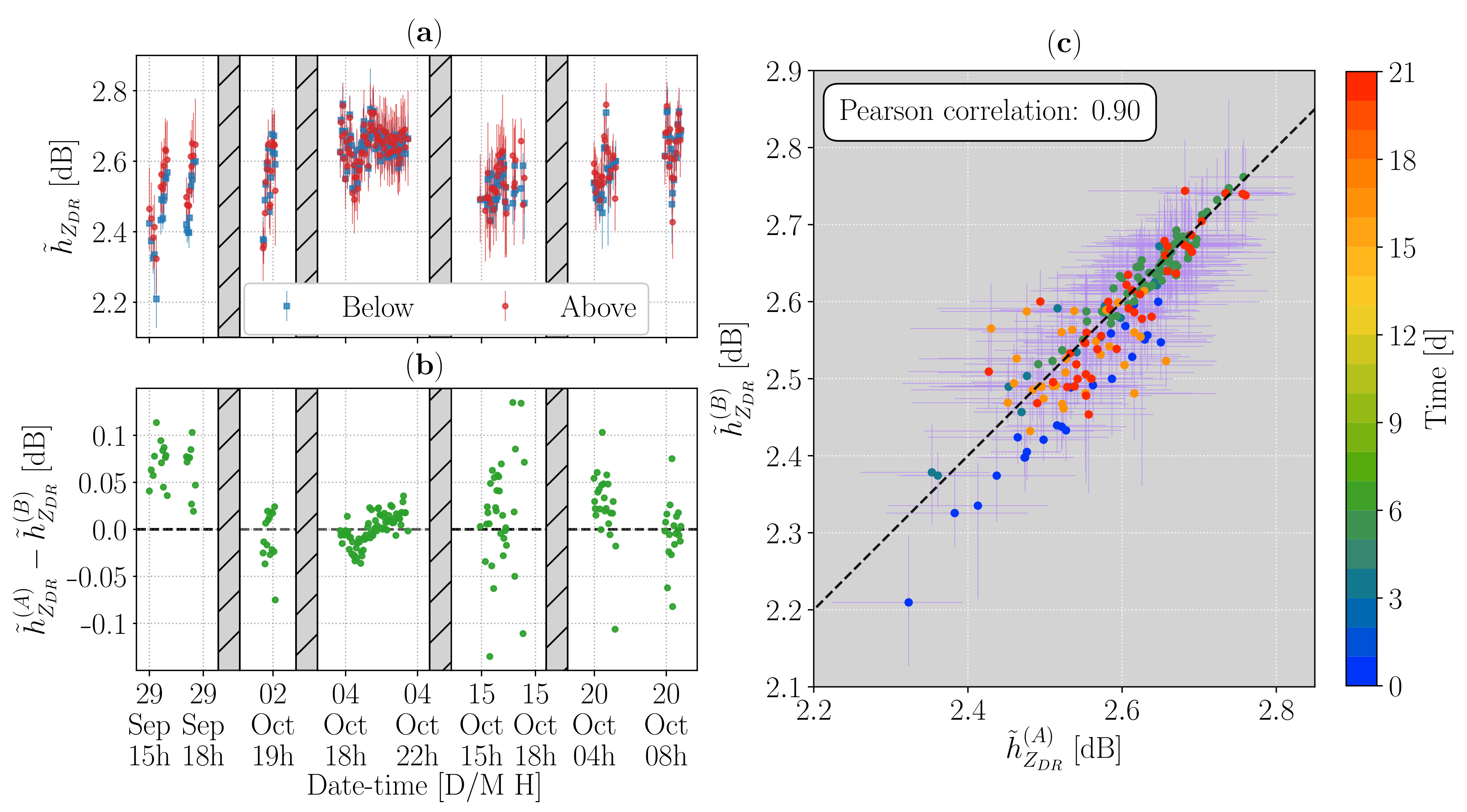
3.2. Median Differential Reflectivity below and above the Melting Layer
Before proceeding with the second part of the algorithm, we deemed it necessary to verify that computing the median of the
values over a region of our profiles dominated by solid hydrometeors gave results comparable to the ones obtainable using data collected in rain. As anticipated in
Section 1, we decided to test this hypothesis to strengthen the basis on which the algorithm was founded and to quantify the agreement between measurements from the two media.
During the HYMEX campaign, we have few precipitation events with a high enough melting layer allowing the simultaneous recording of data below and above it, while excluding all range gates closer than 1500 m to the radar, a threshold manually chosen to fully exclude any contamination from the extreme values at low altitudes due to aging TR limiters.
After imposing the same conditions on
,
and
as in
Section 3.1, and after limiting
between 0 and 20 dBZ, we identified the center of the bright band as the running average, with a centered window, over 20 scans (approximately 1 h and 40 min) of the previously defined
. All measurements at less than 500 m from this central height were excluded, delimiting a buffer zone to exclude radar volumes containing both solid and liquid precipitation. Finally, on the remaining sections each scan, we computed the median of the differential reflectivity distribution below,
, and above,
, the melting layer. The resulting time series of these median values and their difference are displayed in
Figure 3, panel (
a) and (
b) respectively, while a scatterplot of
against
is presented in panel (
c). The latter, together with the high Pearson correlation coefficient, equal to 0.90, showed a good overall agreement between the two quantities. Only the first precipitation event stands out as being almost always below and relatively far from the dashed line of unit slope and 0 dB intercept, but we could not find any specific cause for this behavior. Looking at the time evolution, it appears that
followed closely
, with their difference below 0.1 dB in most cases. This last value in particular ensures the suitability of measurements collected above the melting layer for the purpose of
calibration since the accuracy required for this application is commonly estimated to be between 0.1 and 0.2 dB [
10,
28].
3.3. Evolution in Time of the Calibration
The second part of our calibration algorithm aimed to capture the temporal variation of
(see
Figure 2) to define a time-varying bias based on the interpolation of the measured median
values. This bias should not be defined only at the exact time of the scans fulfilling the required conditions (see
Section 3.1); but continuously during the campaign, to unambiguously calibrate all measurements. A constant bias on predetermined time intervals, such as daily or hourly calibrations, is not appropriate to avoid discontinuities at the edges of these periods, which could result in artificial jumps in the data series. This problem can be avoided by setting the bias equal to the running average of the median
values. However, this solution introduced a high degree of arbitrariness in choosing the window for the average, and in deciding whether its extension should vary across campaigns. Instead, we looked for an alternative in which the temporal dependence was dictated mainly by the data themselves.
Among the existing interpolation techniques we selected ordinary kriging [
24] (pp. 119–120) because it is the best linear, unbiased estimator (for Gaussian random functions). The underlying hypothesis is that the
calibration offset is Gaussian and stationary in time.
Even though the technique is classically used with spatial data, it can also be used with temporal data [
24] (pp. 105–106), as in our case. Examples of application of this technique to radar meteorology can be found in References [
29,
30,
31]. The implementation used in this study is the one from the Python kriging toolkit [
32].
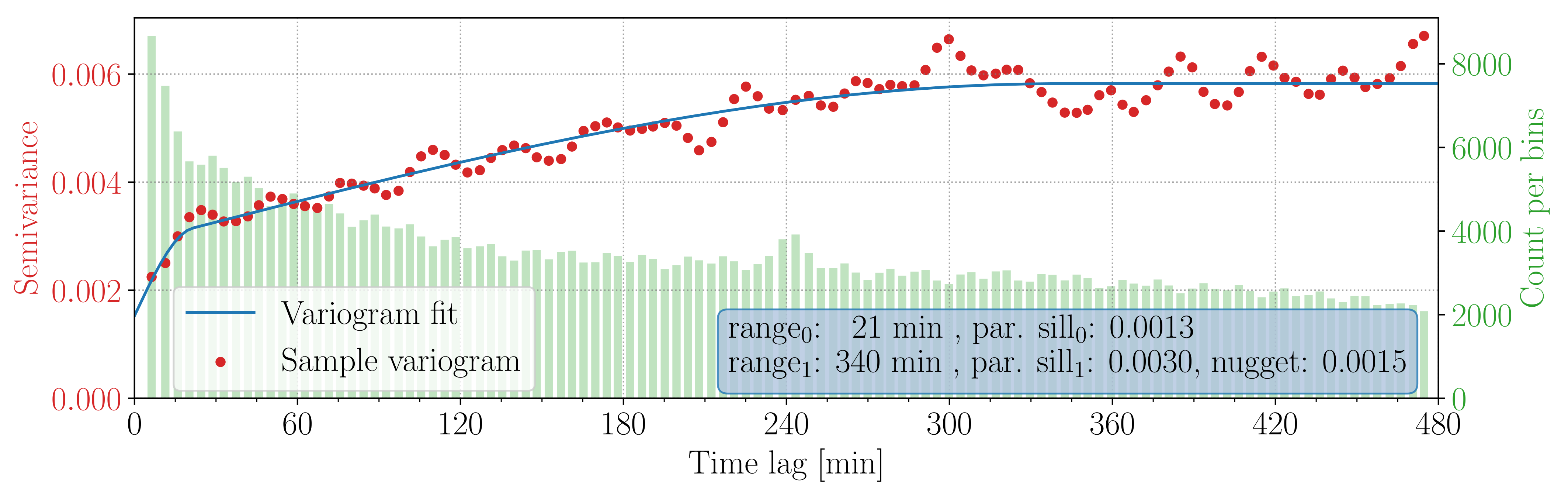
We started the analysis by computing the sample semi-variogram, using the Matheron estimator [
24] (p. 69), shown in
Figure 4. The semi-variogram was defined as half the variance of the increments of a random function [
24] (p. 58), and it quantified the spatial similarity between measurements at different distance lags. Since the whole time series spanned almost 2 months, it was necessary to limit the maximum time lag to a realistic amount, limiting the dependence of the final correction on a scan from what happened too far in time. This threshold differed across campaigns, and in this case we fixed it to 8 h, where the sample variogram seemed to have flattened and remains approximately constant for a few hours.
The interpolation by ordinary kriging required in input a variogram model, which needed to be fitted to the sample variogram. For PAYERNE we decided to use the sum of two spherical models [
24] (p. 61) plus a nugget, since the sum of valid models is valid in turn. The fitted function and its parameters are shown in
Figure 4: combining the two models appeared to capture reasonably well both the sharp rise in the semi-variance in the time lags below 30 min and the slower increase spanning the following lags up to approximately 6 h. This variogram fit, together with the date-times
and their respective median
values, allowed us to finally apply ordinary kriging, which provided us with the linear combination coefficients that we used to estimate the calibration bias at arbitrary date-times during the campaign.
Since the type of variogram model was dictated by the sample variogram, the choice differed for other datasets. We used a spherical one for VALAIS, a Gaussian one for HYMEX and the second part of APRES3, and the sum of a spherical and a gaussian one for the first part of APRES3. In all cases, a non-zero (but relatively small) nugget was present, indicating a limited variability at temporal scales below 5 min. The total range (considering the longest one in case of sum of models) varied between 340 min and 720 min.
4. Results
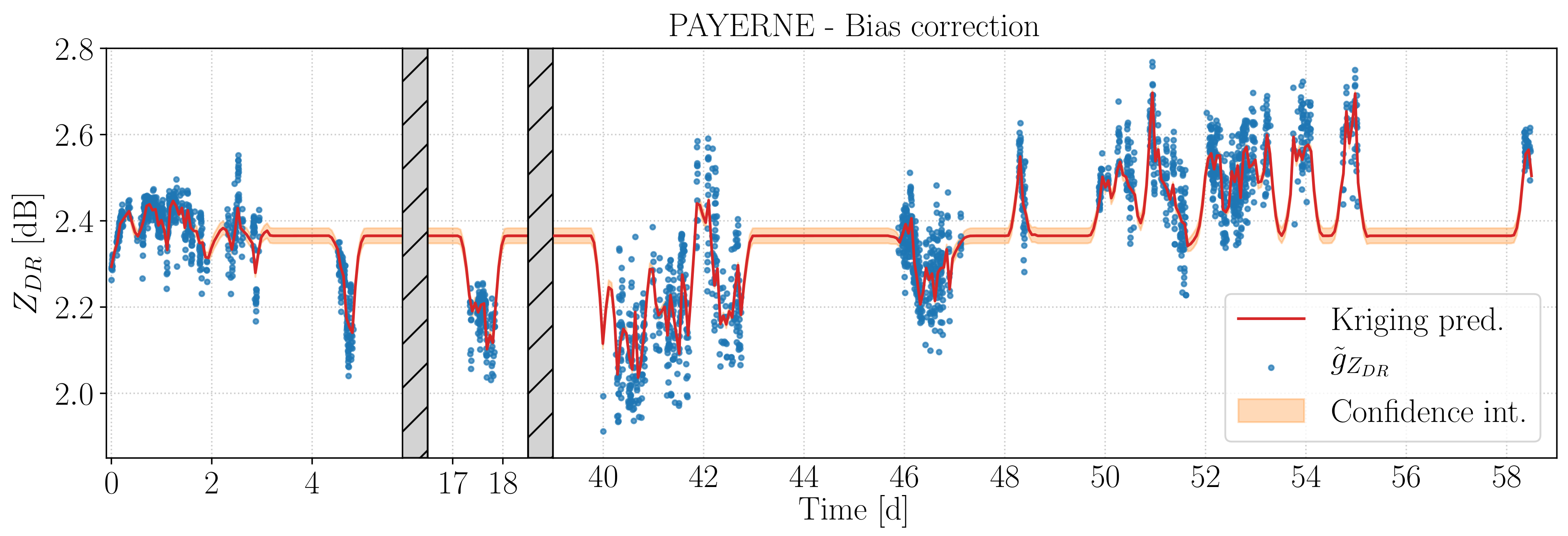
For the PAYERNE campaign, the evolution in time of the calibration bias obtained as described above is displayed in
Figure 5, where it was computed over 1000 equally spaced points across the time span of the campaign. At first glance, it seems that the kriging interpolation followed the general trend of the input
, without fluctuating rapidly between each of them. In reality, since a nugget was present in the variogram model provided to kriging, the interpolation was an exact one, but the curve was allowed to be discontinue at the input coordinate. The behavior was similar to what we would have obtained in using kriging over data with uncertainty, but with the advantage of not being obliged to provide the uncertainty a priori. Instead, a similar role is played by the nugget, resulting from the variogram model fit of
Section 3.3. A clear disadvantage of this approach was the extra difficulty in calibrating the original PPI scans at 90
elevation: rather than using the discontinuous value, equal to
, we substituted it with the average between the bias computed via kriging 1 s before and after
, to enforce a better consistency with the calibration of the other scans. We decided to set the time shift equal to 1 s as it was an arbitrarily small interval over which the curve would not change significantly, while allowing us to avoid the discontinuity.
An additional benefit of defining the bias using a kriging interpolation was the automatic computation of the standard deviation of the estimate, which we multiplied by three to obtain the final confidence interval. The interval increased the further we went away from the input , while the bias moved toward the average value for the campaign. This behavior resulted in a more “classical” calibration of precipitation events that for any reason (lack of vertical extent, for example) lacked input , which would therefore receive a constant, average bias. The transition to this average was smooth and relatively slow, depending on the variogram model used. Thus, no abrupt changes were observed after one of the precipitation events used to compute the calibration finished its passage above the radar, and residual precipitation recorded soon afterward further away from the radar was not immediately calibrated using the average bias.
4.1. Evaluation of the Calibration
We already discussed in
Section 3.2 the similarity between the median
values obtained above and below the melting layer in a series of PPI scans at 90
elevation. While the comparison results confirmed the suitability of the
as the basis for the calibration, the result of the kriging interpolation still needed to be tested. As we anticipated in
Section 2, we had access for the PAYERNE campaign to the data collected by a second radar, called DX50. So, for a first evaluation of the calibration, we decided to compare the overlapping RHI scans before and after subtracting the bias from the
field.
4.1.1. Calibration of Dx50
The first step was the computation of the calibration for DX50, which will follow similar steps to the MXPol case, with some minor modifications to accommodate the differences in the dataset. To compensate for the absence of
and
, we introduced a condition on the reflectivity factor for horizontal polarization, imposing
dBZ. This greatly reduced the noise in the dataset, and it also eliminated the strong asymmetry in the distributions
, which were skewed towards positive differential reflectivity values, as visible in the grayscale 2-dimensional histogram of the
couples in
Figure 6, panel (
a). Additionally, we reduced the threshold on
, setting it equal to 100, since the
values recorded at each range are an average over the 360
rotation (see
Section 2). As a consequence, the total number of data points available for the analysis was relatively low. The selected region of the profiles suitable for extracting the median values
showed an interesting behavior, with two separated modes in the 2-dimensional histogram, shown in color in
Figure 6, panel (
a). Before proceeding to the interpolation by kriging, we also lowered the threshold on the number of remaining valid measurements per scan at each
, setting it equal to 10. The final bias for DX50 is displayed in
Figure 6, panel (
b). Interestingly, the central
value of the two modes of panel (
a) appeared as attractors around which the calibration of few events oscillates, and the passage from one to the other happened sporadically. We do not have any plausible explanation for such a behavior.
Between precipitation events, the interpolation by ordinary kriging fell back to the average value for the campaign, which differed from the two attractors by approximately 0.2 dB. If a hypothetical shallow event, not used as input and with an unknown real bias oscillating around one of the attractors, was calibrated using this average value, the error would still be considered below acceptable accuracy threshold required for most tasks, estimated to be around 0.2 dB [
10].
4.1.2. Comparison of Overlapping Rhi Scans
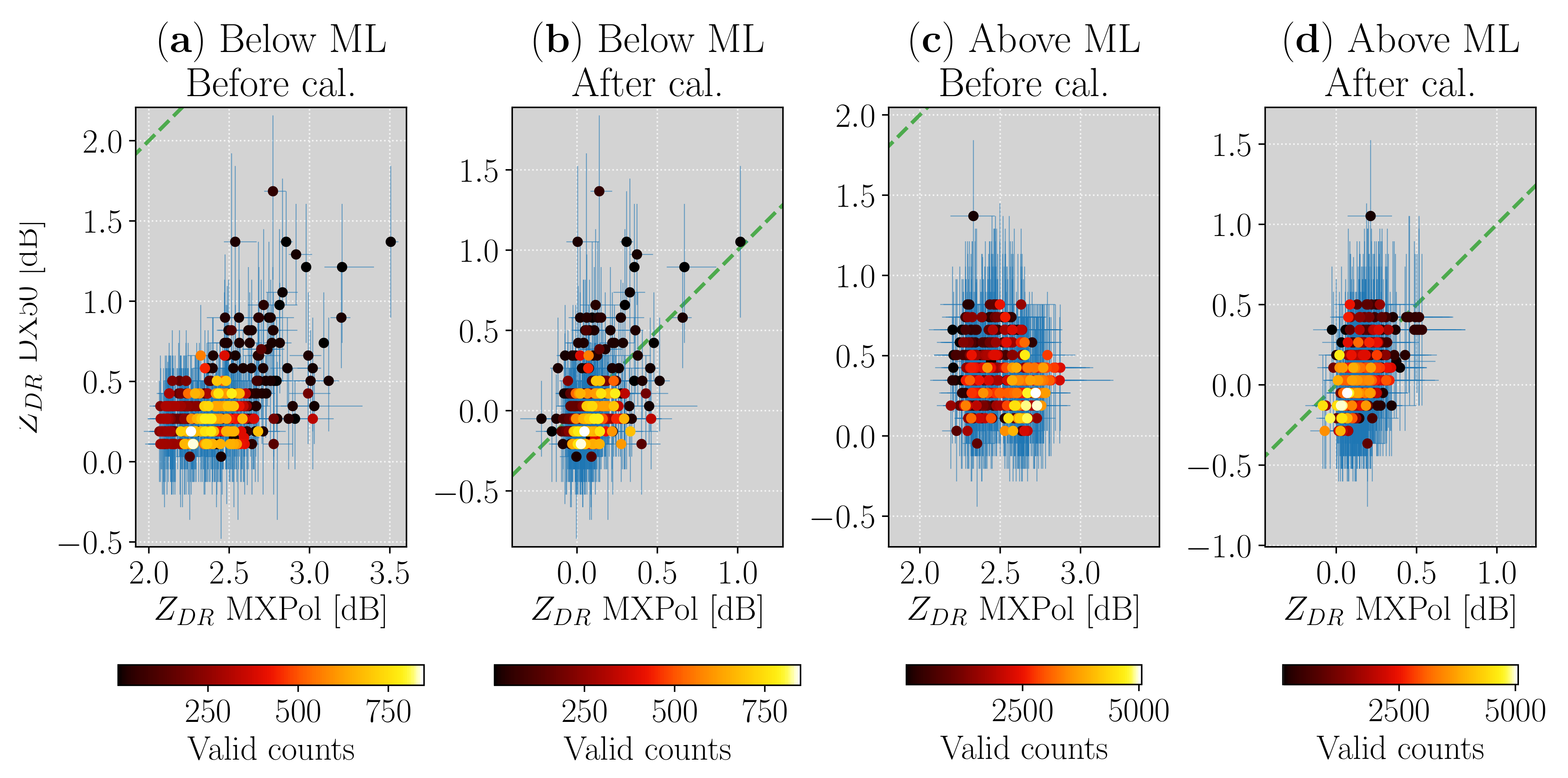
For the actual comparison of overlapping RHI scans, we could not perform a volume by volume comparison, since no pair with similar spatial position and elevation angle could be found. Given their proximity, interferences strongly affected the measurements of both radars, since the two operate at the same frequency. These artifacts are more visible at lower elevations, especially in MXPol, whose measurements below 22 elevation had to be removed. This strongly limits the selection of volumes suitable for the volume by volume comparison. Therefore, we followed a different approach, by comparing median values in analogous regions in the two overlapping RHI scans.
First, we selected a region for the comparison, by imposing the following conditions:
elevation angle between 23 and 53,
height above the ground between 250 m and 5000 m,
minimum distance from the origin radar equal to 1300 m for MXPol, and 600 m for DX50.
The discrepancy in the last threshold is due to the aging of the TR limiter of MXPol, which increases the number of unavailable gates for low r. As in previous subsections, we imposed some thresholds on the polarimetric variables:
, to enforce the homogeneity of the considered volumes,
dBZ and dBZ, to exclude particularly strong or weak return signals.
We also imposed a threshold of 5 dB on both and for MXPol. Given the unavailability of in the DX50 data files, the same threshold could not be applied to the latter.
This filtering was followed by an identification of the melting layer, using
, and adopting an approach analogous to the one described in
Section 3.2. By dividing the measurements above and below it, we obtained two distributions per scan for each radar, of which we could compute the median and the quantiles
and
. This division was motivated by the need to compare analogous regions in the MXPol and DX50 measurements. After matching each RHI scan from one radar with the one closest in time from the other, with a maximum interval of 5 min, we examined the agreement between their median values before and after applying the calibration.
The first comparison, based on the scatterplot of median
values before and after the calibration, is presented in
Appendix A. Even though the results showed a reduction of the overall bias between the two radars, the impact of the temporal variability of the calibration was not clearly visible. Therefore, we decided to proceed with a second comparison, shown in
Figure 7, focusing solely on monitoring the difference between the median
values of the two radars in time. The median value of these differences decreased after the calibration, and this reduction was accompanied by an improved consistency of the statistics below and above the melting layer. Before the bias was subtracted, these median values were equal to 2.0 dB (below) and 2.1 dB (above), while their corresponding values in the bottom panel were both equal to 0.1 dB. Thus, the results were within the required accuracy of the calibration, estimated to be 0.2 dB for most applications [
10]
Additionally, the distributions of the differences (shown on the right side of each panel) were narrower after the bias removal, with a decrease in the interquartile range of approximately 0.1 (below) and 0.2 (above). The change was likely caused by a less marked evolution in time of the differences in the bottom panels when compared to the top ones. We interpret this improvement as a benefit of the time-varying calibration, able to account for the independent changes of bias in the two radars.
4.2. Calibration of the HYMEX, VALAIS and APRES3 Campaigns
The same calibration method used for the PAYERNE campaign was applied to the other datasets listed in
Section 2, with the sole exception of DAVOS, which requires a more in-depth analysis.
Figure 8 provides the original 2-dimensional histogram and the selected section of the profiles in the panels on the left side, accompanied on the right side by a display of the time evolution of the final bias, computed over 1000 points equally spaced across the time spans of the campaigns. The APRES3 dataset was divided into two parts to account for a change in the scanning parameters, which affected some variables fundamental for the algorithm, such as position and spacing of the range gates.
A close look at the 2-dimensional histograms immediately reveals that their vertical extent varied by several km, as a result of the different nature of the precipitation events recorded at the different locations. Focusing on the x-axis, the VALAIS campaign had a distinct enlargement of the range of values spanned by the selected section of the histogram. We also observed an interesting behavior in the lower half of the HYMEX histogram, where the central part with a higher measurement count shifted slightly to the left. Despite the heterogeneity, the first part of the calibration algorithm consistently identified a sufficiently homogeneous region of the profile, mostly unaffected by the issue of the lowest range gates where extreme values were recorded, as hinted by the grayscale 2-dimensional histograms.
The large differences in the temporal evolution (right-side panels) can partially be attributed to the different time intervals covered in each plot. While HYMEX spanned approximately 2 months, for VALAIS we only had valid measurements for a week. Remaining discrepancies in how the calibration fitted the measurements are mainly the result of the diverse variogram models used for the kriging interpolation. For example, the Gaussian variogram adopted for the APRES3 campaign produced a particularly smooth curve, as opposed to the spherical one of VALAIS that caused more high-frequency fluctuations in the bias, despite the comparable range of the two and the similar time span of the campaigns. Even when present, these fluctuations seemed to be of an amplitude smaller than 0.1 dB. This amount is below the accepted accuracy threshold, and significantly smaller than the discrepancy between the median values and what the calibration would have been if we ignored its time dependence and assumed a constant bias.
In several campaigns (including DAVOS, presented in the next subsection), significant variations of the median values, up to 0.8 dB, can occur in relatively short time spans, ranging from few hours to a day. We suspect that it may be due to variations in the temperature of the radar system or to wet radome effects.
4.3. Calibration of the DAVOS Campaign
The temporal evolution of the median values for the DAVOS campaign showed a downward trend that could not be properly handled by the ordinary kriging interpolation (which assumes stationarity). Defining a bias that returns to its average value at coordinates far enough from the original data points would result in large fluctuations at the beginning and the end of the series. Therefore, we decided to split the dataset into three parts, in which the trend appears negligible and the median seems to fluctuate around a common average value.
To calibrate the three intervals, we treated them as separate campaigns for everything that concerns the kriging interpolations. First, we computed the variogram and fitted a model on each of them, and then we used kriging to determine the temporal evolution of the bias, displayed in
Figure 9. Each panel shows the results for one of the intervals, superimposed to the original differential reflectivity values from which the calibration has been derived.
The average bias was close to 3 dB for the first panel, and it dropped to less than 2.5 dB in the last. The curve deviated from this central value for less than 0.2 dB in most cases, which suggests that a precipitation event calibrated with the average bias would likely receive a calibration of sufficient accuracy, at the best of the available knowledge. In contrast, an application of the ordinary kriging interpolation on the whole DAVOS dataset would result in a significantly larger distance between the average calibration and the bias in the proximity of the original median values. In some cases the difference between the two would have a magnitude of over 0.5 dB, with the calibration curve oscillating between the two values in a span of few days. The average bias, therefore, would likely become not representative of the real one, at least for precipitation events far enough in time from the original PPI scans and at the extremes of the campaign.
4.4. Effects of the Calibration on the PPI Scans
Once the calibration procedure was applied to all campaigns, its influence on the empirical probability density function of the differential reflectivity values recorded in the PPI scans at 90 elevation could be investigated. Only the relatively homogeneous region suitable to apply the correction was considered, to limit the impact on the statistics of non-physical measurements in the lowest range gates.
As anticipated at the beginning of the section, it was necessary to choose the bias at an arbitrarily small time shift to calibrate the vertical PPI. The aim was to avoid the large and unrealistic variability at small scales at those locations, caused by the exact and discontinuous nature of the kriging interpolation. We decided to average the values obtained 1 s before and after the time of the scan, using the result for the calibration. The bias could be considered effectively constant over this interval, given the relatively long time scale over which it normally varied, as highlighted by the variograms.
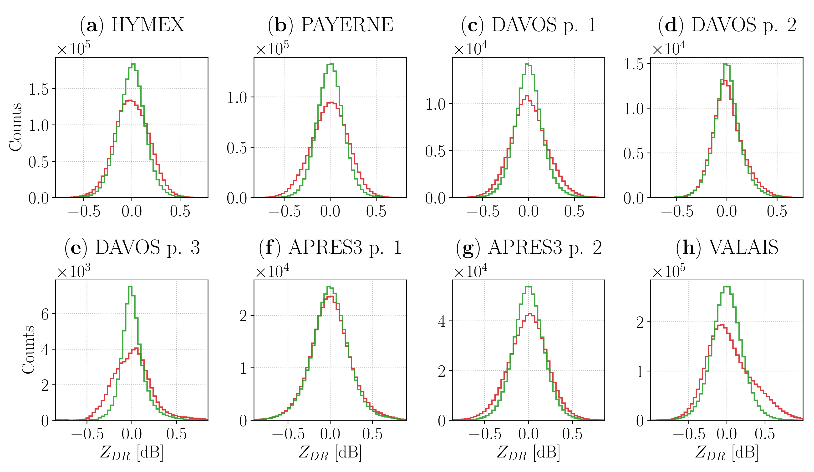
A quick way to visualize how the
empirical distributions evolve after the calibration was through the superposition of histograms, centered around their median value. As expected, the comparisons displayed in the eight panels of
Figure 10 revealed a narrowing effect of the time-varying bias, accompanied by an increase in the symmetry of the calibrated histogram for VALAIS and the third part of the DAVOS campaign.
The extent of these two effects varied across campaigns, and it can be better appreciated by looking at some simple statistics associated with the aforementioned empirical distributions. Thus, we provide in
Table 2 their median and interquartile range (IQR) before and after the bias is subtracted from the
fields.
Although the magnitude of the decrease in interquartile range, usually less than 0.1 dB, was relatively small in absolute terms, its importance in percentage terms was more remarkable, being close to 20% in most cases, with few exceptions such as the last part of DAVOS (approximately 45%) and the first part of APRES3 1 (close to 6%). Given how the calibration was defined, the median values after its application were much closer to 0 dB that the original counterparts. While this result is not surprising, it indicates that the usage of the kriging interpolation in the proximity of the scans did not significantly bias the empirical distribution. For completeness, subtracting the exact interpolation from the scans would have resulted in both median and IQR being equal to 0 dB.
5. Summary and Conclusions
The proposed technique for differential reflectivity calibration is based on the kriging interpolation of the median value of automatically selected regions of vertical PPI scans. It has been applied on the measurements collected during five field campaigns, remarkably diverse in terms of location, season and typology of precipitation events observed. While hybrid techniques, requiring modest changes in hardware, already exist and provide acceptable results, many commercial polarimetric radars do not have an automatic end of volume scan calibration. The method proposed in this study is suitable for these radars.
The algorithm is designed to function with profiles including only liquid precipitation, only solid or both, even though in the last case the measurements from the melting layer are excluded. Therefore, the first topic investigated in the current study is the suitability of data collected in snow and ice for calibration purposes. The underlying assumption is that the uneven returns on the horizontal and vertical polarization channels, due to the irregular shapes of ice particles, are compensated, in average and over a large enough data pool, by the randomness of their orientation and by the full azimuthal rotation. This hypothesis has been tested in
Section 3.2, where the comparison of measurements from below and above the melting layer from five precipitation events of the HYMEX campaign yielded a satisfactory agreement, both in terms of correlation and absolute difference. The
values in light rain, observed through PPI scan at 90
elevation, have been widely used in the scientific literature for differential reflectivity calibration, and the similarity found in the comparison hints towards the eligibility of analogous measurements of solid hydrometeors for the same purposes.
The number of range gates affected by the aging of the TR limiter (but it could be any other issue affecting ) changes across the various datasets, and for this reason, we developed a simple algorithm for the automatic identification of a relatively homogeneous region of the profiles, by thresholding some statistics derived from the empirical probability density function of . A series of controls removes from the dataset the scans with too few measurements or that are too far apart in time, and the median of the remaining differential reflectivity values constitutes the input for the ordinary kriging interpolation. The latter provides the calibration bias and its uncertainty, based on the fitted variogram which describes the temporal structure of the bias. Despite a degree of arbitrariness in picking the function for the fit and in deciding the maximum realistic time lag, the interpolation is mostly decided by the information already available in the data, solving the problem of choosing how to calibrate measurements in between the appropriate vertical PPI scans. As long as the fit follows the empirical variogram, the differences between the possible models are usually orders of magnitude smaller than the fluctuations in the interpolated data, and surely below the desired accuracy threshold.
Additionally, the usage of a non-zero nugget in the variogram models results in a relatively slow variation of the bias curve. In this way, the undesirable rapid fluctuations needed for an exact and always continuous interpolation are avoided and substituted by a discontinuous curve, which evolves smoothly, without rising or falling too steeply, everywhere except at coordinates of the input PPI scans, the only moments of discontinuity that allow the interpolation to remain exact. However, this behavior complicates the calibration of these PPI scans, for which we adopted a workaround, consisting in using the average of the biases at an arbitrarily small interval before and after the scan time. This is clearly a limitation of the method, which could theoretically be addressed by providing to the kriging interpolation an uncertainty on the input median values. The latter could also be allowed to vary during the campaign, resulting in more flexibility in determining how close the curve should be to these inputs. The downside to this approach is the need for determining such uncertainty. It would introduce additional space for arbitrary choices and complexity to the algorithm, which we wanted to avoid at this stage.
Both the automated identification of suitable sections of the profiles and the kriging interpolation have been tested by comparing the calibrated
fields from the overlapping RHI scans of two X-band radars during the PAYERNE campaign. The median values recorded below and above the melting layer have been taken into consideration, and in both cases, we observed improvements in the distribution of the differences between the two radars. The approach of their central value to the ideal value of 0 dB has been accompanied by a narrowing of the distributions, likely due to the time dependence of the calibration, even though we did not see a marked rise in the correlation of the measurements of the two radars (likely due to limited
variability and significant noise). Nevertheless, an absolute value close to 0.1 dB for the median value of the differences, accompanied by a more consistent evolution in time, as shown in
Figure 7, already hints towards a sufficient accuracy for the calibration. This agreement also implies a certain degree of resilience of the calibration, considering its adequate functioning on a different radar. In fact, it was successfully applied to DX50, whose measurements differ from the first radar in crucial aspects such as the absence of a noticeable TR limiter aging, or a pronounced asymmetry in the two-dimensional histogram of the couples
.
We also studied how the calibration affects the empirical probability density function of the
measurements in the previously selected homogeneous section of the original PPI scans. In most cases, we observe a reduction of the IQR of these distributions by approximately 20%, accompanied by a significant shift of the median value towards the 0 dB. Since the algorithm is designed to follow the median
values in the same region, this last check has been intended as a confirmation of the correct functioning of the method, rather than a test on the accuracy of the results. In practice, it shows that the non-exact extrapolation from the kriging interpolation used as final bias does not impact negatively these distributions, whose final forms are consistent with what we would expect from a series of calibrated scans, given the hypothesis tested in
Section 3.2.
In the end, the greatest limitation of the proposed method emerges from the difficulties encountered in applying it to relatively long campaigns, like DAVOS. By using ordinary kriging, we implicitly assume that the average of the interpolated quantity remains stationary for the whole period of interest. While this assumption is often true for field campaigns spanning only a few weeks, a distinct trend was visible for the DAVOS dataset, which had to be split into three separate regions to adequately satisfy the hypothesis.
A solution to this problem could be the usage of a universal kriging interpolation, which drops the assumption of a constant mean in the studied field [
24] (p. 151). Instead, it assumes that the function to estimate (the
bias in our case) is the sum of a deterministic smooth function, called the drift, and the usual second-order intrinsic random function, as per ordinary kriging. An even more promising prospect would be the employment of a kriging interpolation with external drift, which is able to take into account the input of auxiliary variables. The temperature may likely play a role for this purpose since it has already been linked to the intraday changes in the
bias in previous scientific literature [
12,
21].
However, the addition of external variables in the calibration algorithm may undermine one of the reasons behind its development. Precise measurements of quantity such as the antenna temperature are not always available for past field campaigns, and we designed the method to be usable on the widest selection of our datasets. It relies solely on the polarimetric variables provided by the radar, and this makes it usable as long as there are vertical PPI scans. Ultimately, the ordinary kriging interpolation offers the simplest solution, with the least amount of external input required, adequate for relatively short datasets where the stability condition of the mean is respected.
Finally, future investigations on the proposed method may study the possibility of extending and adapting it to near real-time calibration. By re-computing the variogram at regular time intervals (every day, for example) it may be possible to provide an approximate calibration, whose time dependence would be based on the variability observed in the data collected until that specific point. Obviously, previously calibrated data should be corrected at each iteration, to take in account the additional information included in the new variogram. The significance of the latter at each time lag should increase alongside the availability of new measurements. The stability of this variogram and their significance will likely play a central role in these possible future investigation. At the end of the campaign, the final calibration should be ideally identical to the method proposed in the current study.


