Spatiotemporal Analysis of Vegetation Cover Change in a Large Ephemeral River: Multi-Sensor Fusion of Unmanned Aerial Vehicle (UAV) and Landsat Imagery


Abstract
:1. Introduction
2. Methods
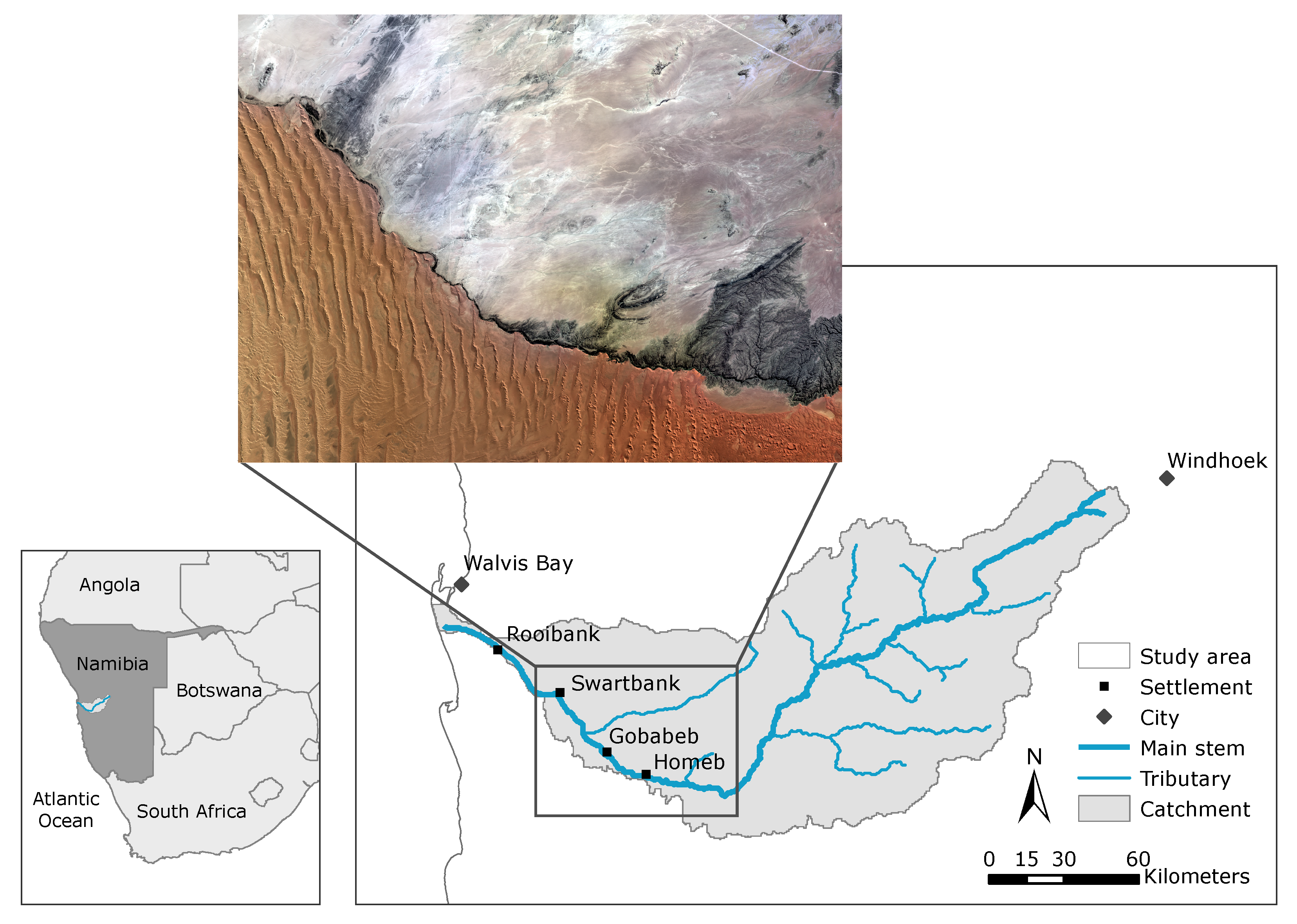
2.1. Study Area
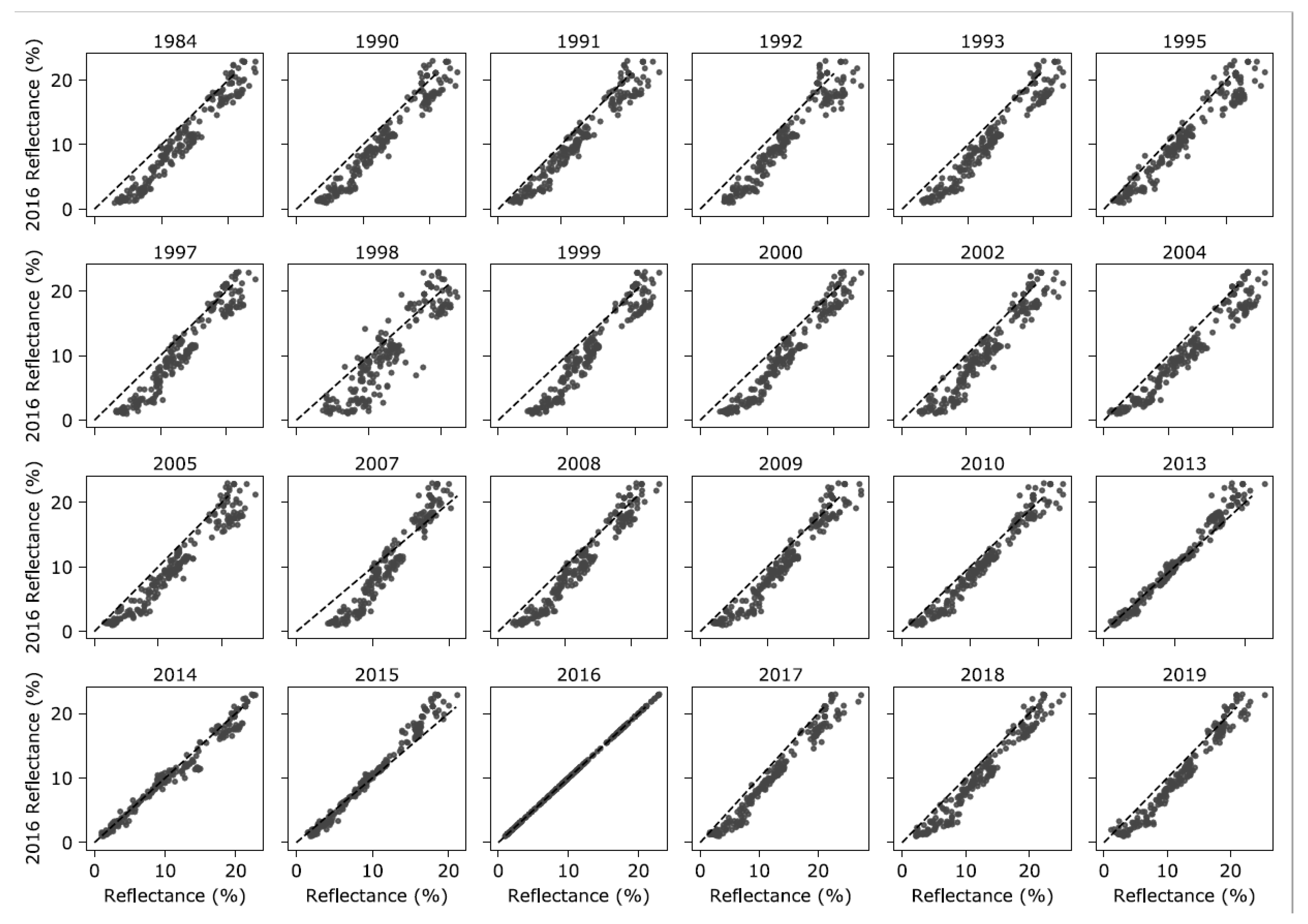
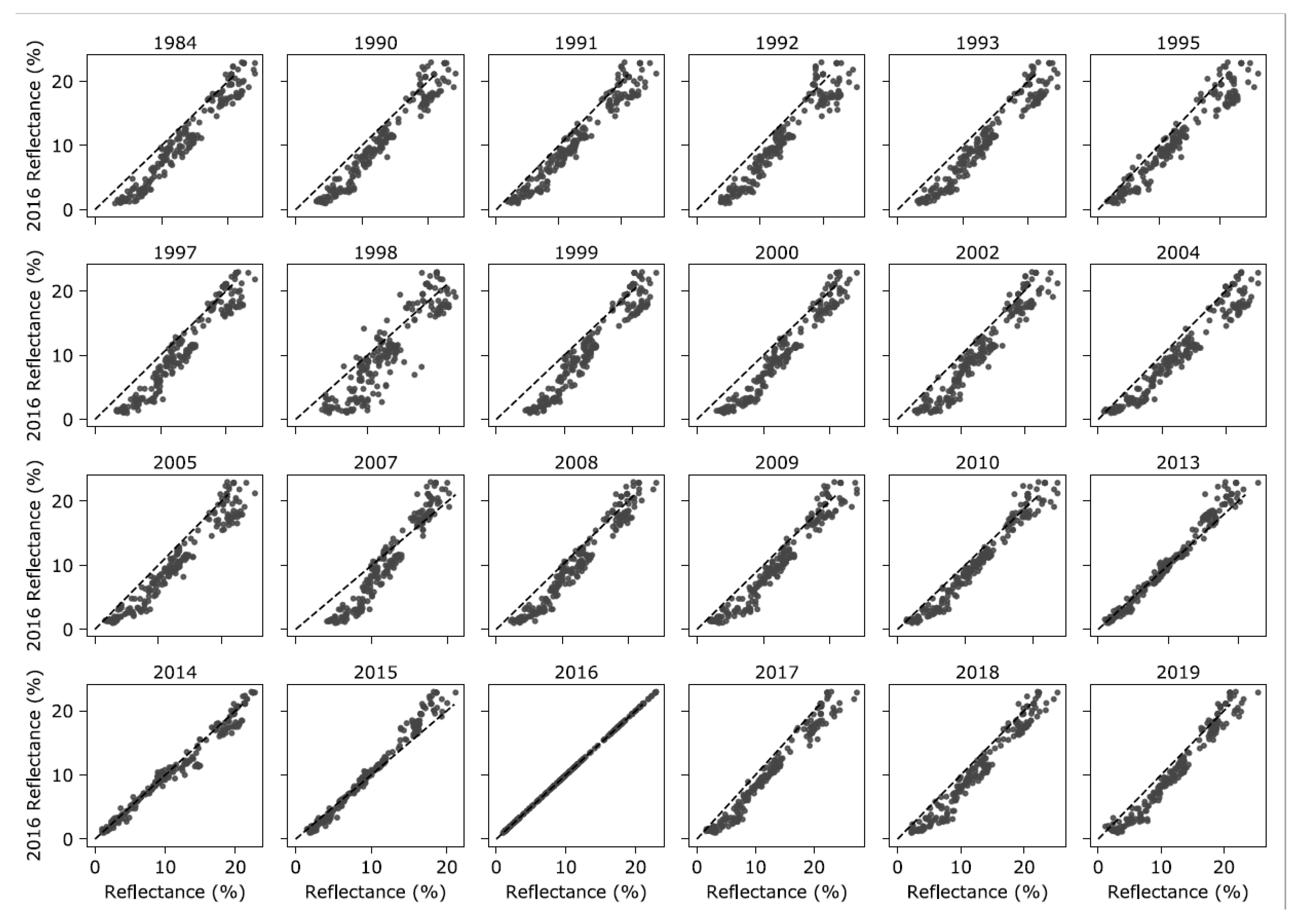
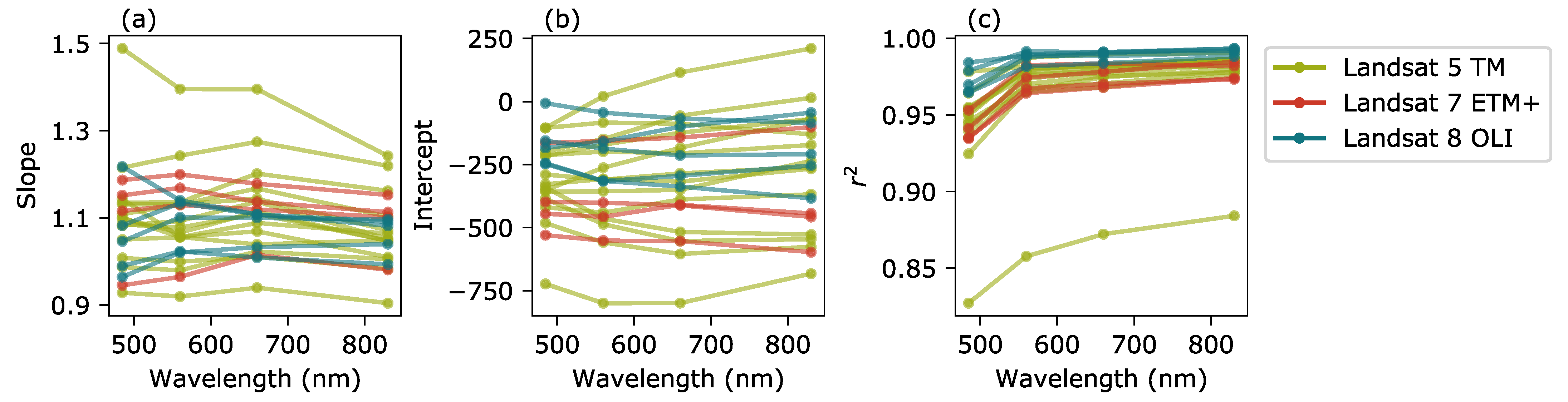
2.2. Intercalibration of Landsat Data
2.3. Aerial Imagery Collection and Processing
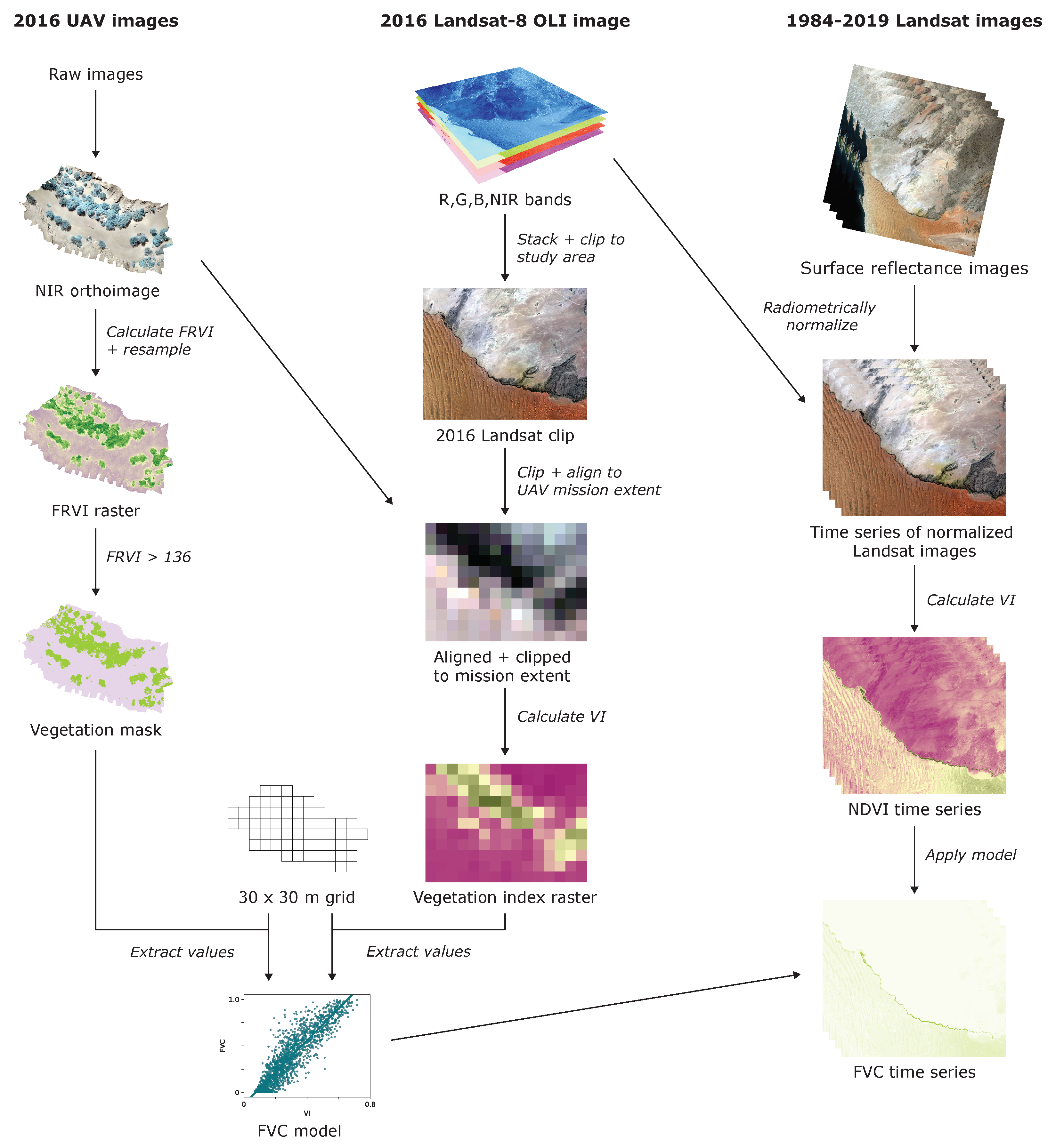
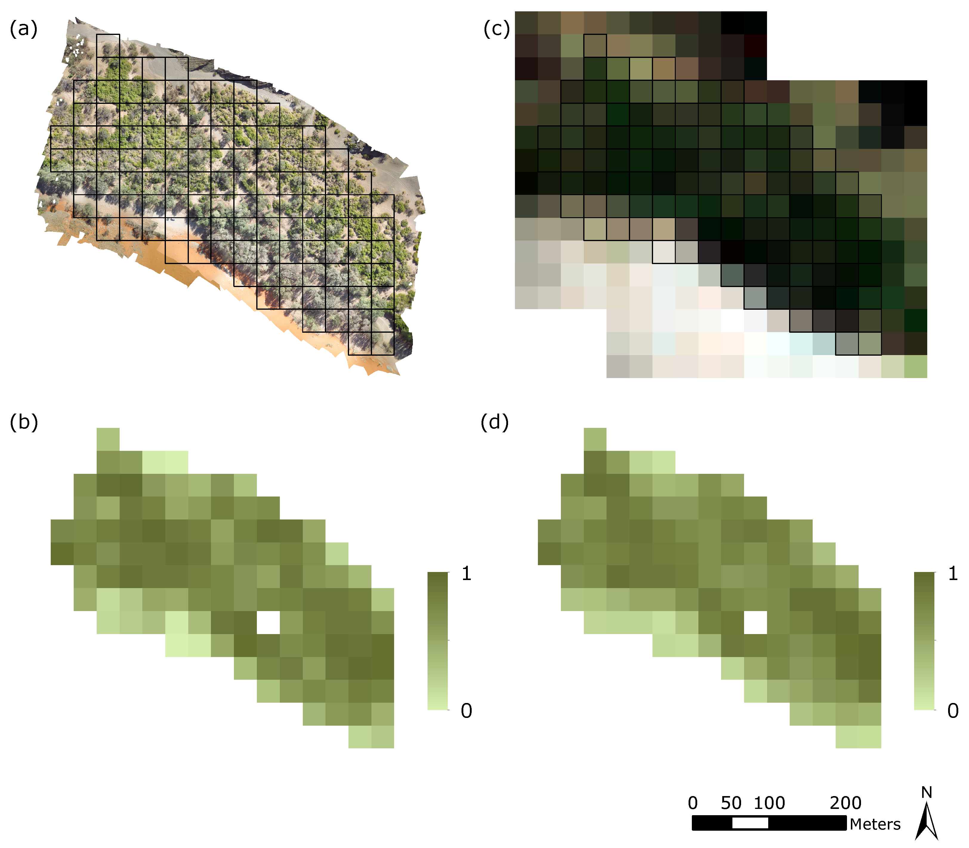
2.4. Calculation of Fractional Vegetation Cover from UAV Imagery
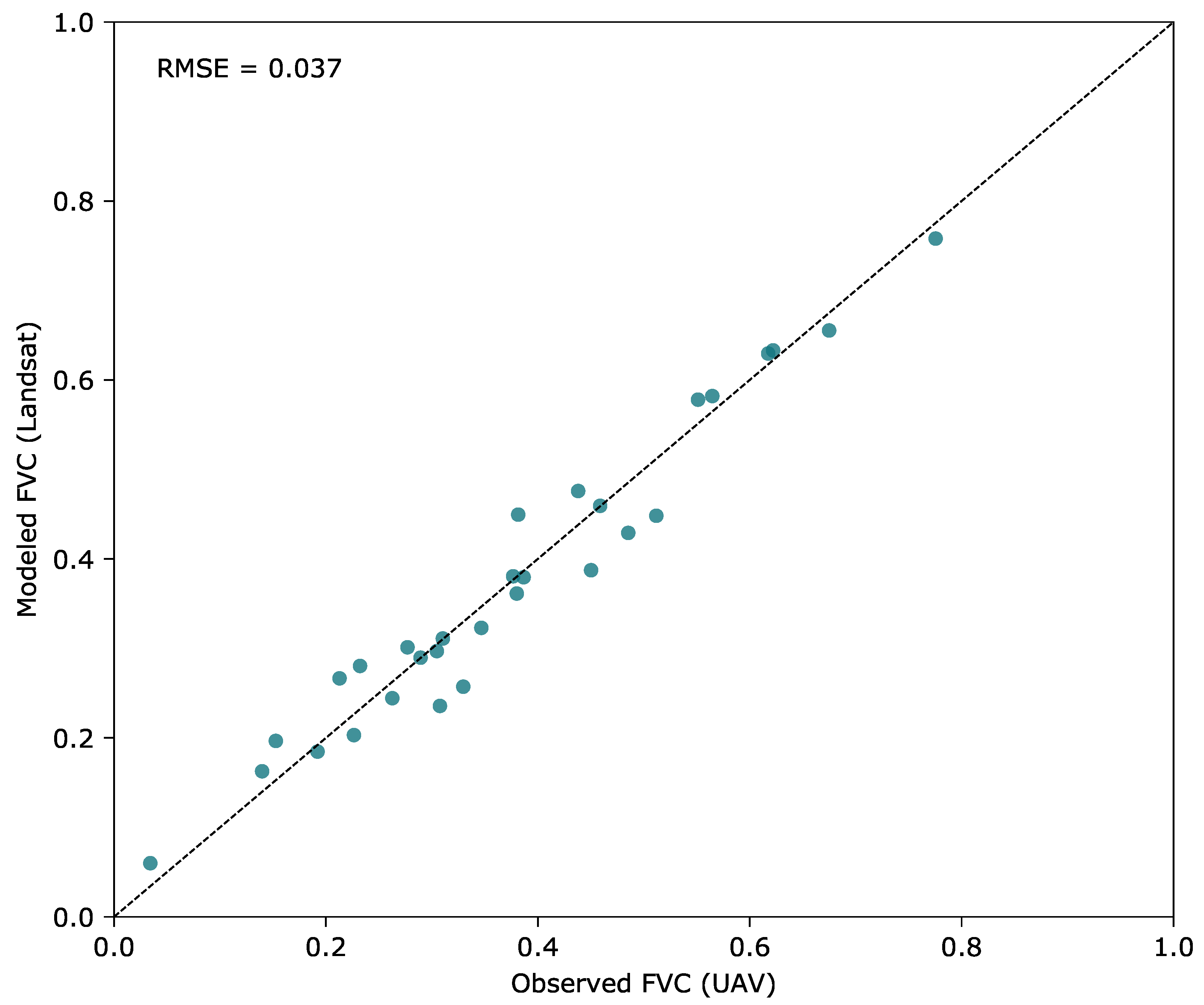
2.5. Calibration of the FVC Model for the Landsat Time Series
2.6. Analysis of Vegetation Cover Change
3. Results
3.1. Intercalibration of Landsat Data
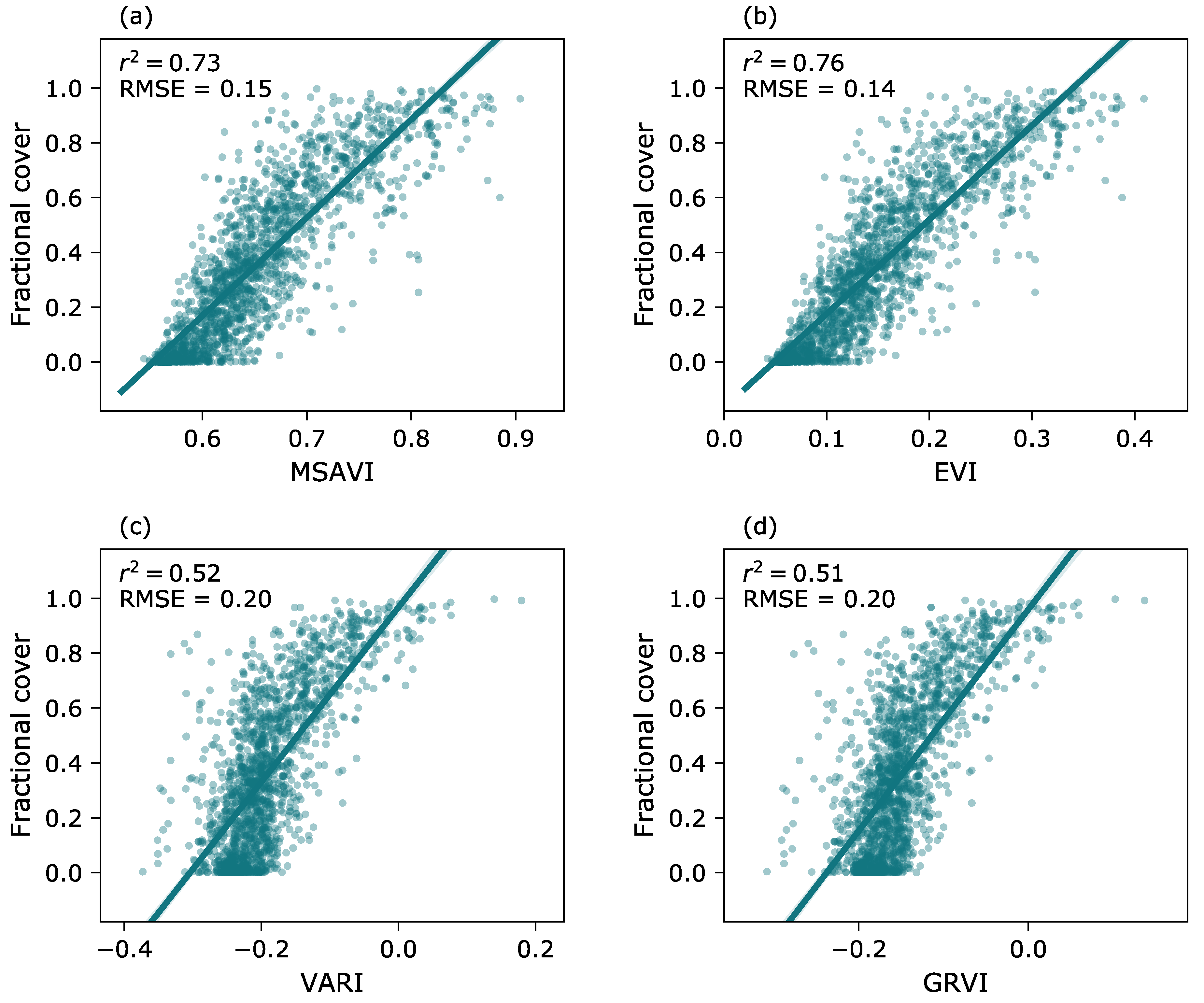
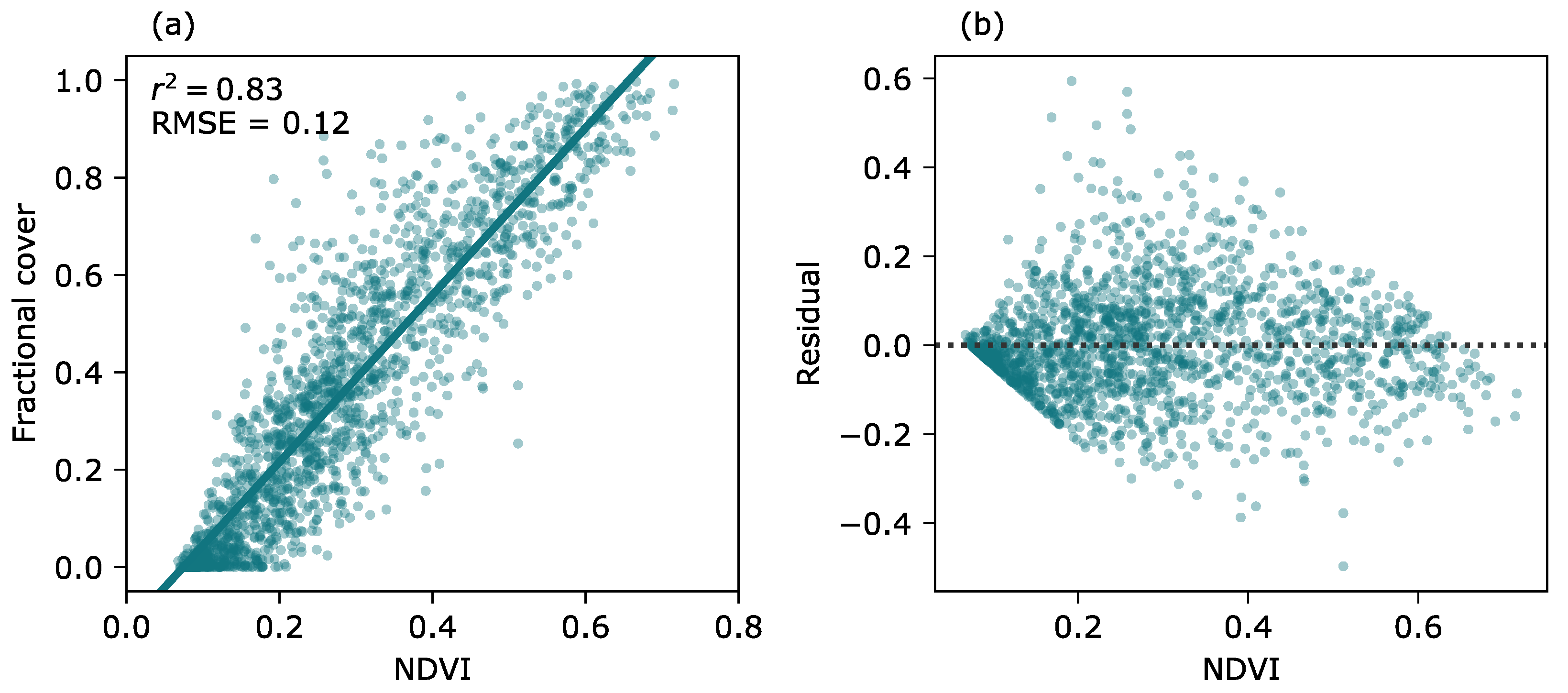
3.2. Modeling of Fractional Vegetation Cover
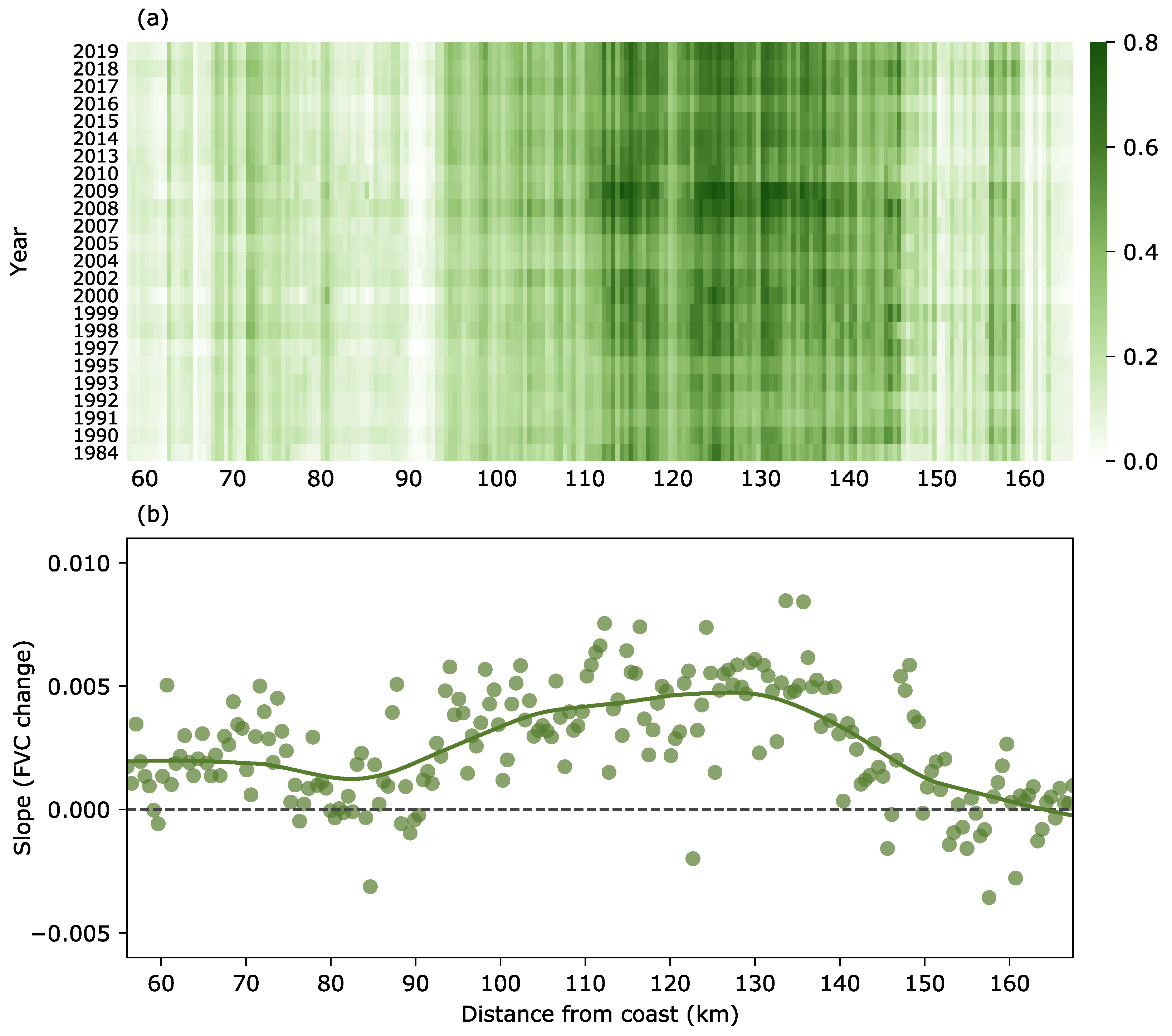
3.3. Change in Fractional Vegetation Cover
4. Discussion
5. Conclusions
Supplementary Materials
Author Contributions
Funding
Data Availability Statement
Acknowledgments
Conflicts of Interest
References
- Gregory, S.V.; Swanson, F.J.; McKee, W.A.; Cummins, K.W. An ecosystem perspective of riparian zones. Bioscience 1991, 41, 540–551. [Google Scholar] [CrossRef]
- Hoffman, M.T.; Rohde, R.F. Rivers Through Time: Historical Changes in the Riparian Vegetation of the Semi-Arid, Winter Rainfall Region of South Africa in Response to Climate and Land Use. J. Hist. Biol. 2011, 44, 59–80. [Google Scholar] [CrossRef] [PubMed]
- Huntley, B.J. The Kuiseb Environment: The Development of a Monitoring Baseline; Technical Report Committee for Terrestrial Ecosystems; Foundation for Research Development: Pretoria, South Africa, 1985; ISBN 0798833971. [Google Scholar]
- Jacobson, P.J.; Jacobson, K.M. Hydrologic controls of physical and ecological processes in Namib Desert ephemeral rivers: Implications for conservation and management. J. Arid Environ. 2013, 93, 80–93. [Google Scholar] [CrossRef]
- Seely, M.K.; Buskirk, W.; Hamilton, W.; Dixon, J. Lower Kuiseb river perennial vegetation survey. J. South West Afr. Sci. Soc. 1981, XXXIV/XXXV, 57–86. [Google Scholar]
- Arnold, S.; Attinger, S.; Frank, K.; Baxter, P.; Possingham, H.; Hildebrandt, A. Ecosystem Management Along Ephemeral Rivers: Trading Off Socio-Economic Water Supply and Vegetation Conservation under Flood Regime Uncertainty. River Res. Appl. 2016, 32, 219–233. [Google Scholar] [CrossRef]
- Datry, T.; Fritz, K.; Leigh, C. Challenges, developments and perspectives in intermittent river ecology. Freshw. Biol. 2016, 61, 1171–1180. [Google Scholar] [CrossRef] [Green Version]
- Nilsson, C.; Svedmark, M. Basic principles and ecological consequences of changing water regimes: Riparian plant communities. Environ. Manag. 2002, 30, 468–480. [Google Scholar] [CrossRef]
- Stromberg, J.C.; Hazelton, A.F.; White, M.S. Plant species richness in ephemeral and perennial reaches of a dryland river. Biodivers. Conserv. 2009, 18, 663–677. [Google Scholar] [CrossRef]
- D’Odorico, P.; Porporato, A. (Eds.) Dryland Ecohydrology, 1st ed.; Springer: Dordrecht, The Netherlands, 2006; pp. 1–341. [Google Scholar] [CrossRef] [Green Version]
- Friedman, J.M.; Lee, V.J. Extreme floods, channel change, and riparian forests along ephemeral streams. Ecol. Monogr. 2002, 72, 409–425. [Google Scholar] [CrossRef]
- McCluney, K.E.; Belnap, J.; Collins, S.L.; González, A.L.; Hagen, E.M.; Nathaniel Holland, J.; Kotler, B.P.; Maestre, F.T.; Smith, S.D.; Wolf, B.O. Shifting species interactions in terrestrial dryland ecosystems under altered water availability and climate change. Biol. Rev. 2012, 87, 563–582. [Google Scholar] [CrossRef] [Green Version]
- Stromberg, J.C.; McCluney, K.E.; Dixon, M.D.; Meixner, T. Dryland riparian ecosystems in the American Southwest: Sensitivity and resilience to climatic extremes. Ecosystems 2013, 16, 411–415. [Google Scholar] [CrossRef]
- Allsopp, N.; Gaika, L.; Knight, R.; Monakisi, C.; Hoffman, M.T. The impact of heavy grazing on an ephemeral river system in the succulent karoo, South Africa. J. Arid Environ. 2007, 71, 82–96. [Google Scholar] [CrossRef]
- Belsky, A.J.; Matzke, A.; Uselman, S.C.N. Survey of livestock influences on stream and riparian ecosystems in the western United States. J. Soil Water Conserv. 1999, 54, 419–431. [Google Scholar]
- Moser-Nørgaard, P.M.; Denich, M. Influence of livestock on the regeneration of fodder trees along ephemeral rivers of Namibia. J. Arid Environ. 2011, 75, 371–376. [Google Scholar] [CrossRef]
- Sarr, D.A. Riparian livestock exclosure research in the Western United States: A critique and some recommendations. Environ. Manag. 2002, 30, 516–526. [Google Scholar] [CrossRef]
- Douglas, C.M.S.; Pettorelli, N.; Mulligan, M.; Henschel, J.R.; Harrison, X.A.; Cowlishaw, G. Widespread dieback of riparian trees on a dammed ephemeral river and evidence of local mitigation by tributary flows. PeerJ 2016, 4, e2622. [Google Scholar] [CrossRef] [Green Version]
- Schachtschneider, K.; February, E.C. Impact of Prosopis invasion on a keystone tree species in the Kalahari Desert. Plant Ecol. 2013, 214, 597–605. [Google Scholar] [CrossRef]
- Shafroth, P.B.; Stromberg, J.C.; Patten, D.T. Riparian vegetation response to altered disturbance and stress regimes. Ecol. Appl. 2012, 12, 107–123. [Google Scholar] [CrossRef]
- Stromberg, J.C.; Merritt, D.M. Riparian plant guilds of ephemeral, intermittent and perennial rivers. Freshw. Biol. 2016, 61, 1259–1275. [Google Scholar] [CrossRef]
- Lite, S.J.; Bagstad, K.J.; Stromberg, J.C. Riparian plant species richness along lateral and longitudinal gradients of water stress and flood disturbance, San Pedro River, Arizona, USA. J. Arid Environ. 2005, 63, 785–813. [Google Scholar] [CrossRef]
- McCoy-Sulentic, M.E.; Kolb, T.E.; Merritt, D.M.; Palmquist, E.C.; Ralston, B.E.; Sarr, D.A. Variation in species-level plant functional traits over wetland indicator status categories. Ecol. Evol. 2017, 7, 3732–3744. [Google Scholar] [CrossRef] [PubMed]
- Francis, R.A. Allogenic and autogenic influences upon riparian vegetation dynamics. Area 2006, 38, 453–464. [Google Scholar] [CrossRef]
- Gurnell, A. Plants as river system engineers. Earth Surf. Process. Landforms 2014, 39, 4–25. [Google Scholar] [CrossRef]
- Sandercock, P.J.; Hooke, J.M.; Mant, J.M. Vegetation in dryland river channels and its interaction with fluvial processes. Prog. Phys. Geogr. 2007, 31, 107–129. [Google Scholar] [CrossRef]
- Jacobson, P.J.; Jacobson, K.M.; Angermeier, P.L.; Cherry, D.S. Hydrologic influences on soil properties along ephemeral rivers in the Namib Desert. J. Arid Environ. 2000, 45, 21–34. [Google Scholar] [CrossRef]
- Abiodun, B.J.; Makhanya, N.; Petja, B.; Abatan, A.A.; Oguntunde, P.G. Future projection of droughts over major river basins in Southern Africa at specific global warming levels. Theor. Appl. Climatol. 2019, 137, 1785–1799. [Google Scholar] [CrossRef]
- Dahan, O.; Tatarsky, B.; Enzel, Y.; Kulls, C.; Seely, M.; Benito, G. Dynamics of flood water infiltration and ground water recharge in hyperarid desert. Ground Water 2008, 46, 450–461. [Google Scholar] [CrossRef]
- Lange, J. Dynamics of transmission losses in a large arid stream channel. J. Hydrol. 2005, 306, 112–126. [Google Scholar] [CrossRef]
- Morin, E.; Grodek, T.; Dahan, O.; Benito, G.; Kulls, C.; Jacoby, Y.; Langenhove, G.V.; Seely, M.; Enzel, Y. Flood routing and alluvial aquifer recharge along the ephemeral arid Kuiseb River, Namibia. J. Hydrol. 2009, 368, 262–275. [Google Scholar] [CrossRef]
- Tooth, S. Process, form and change in dryland rivers: A review of recent research. Earth Sci. Rev. 2000, 51, 67–107. [Google Scholar] [CrossRef]
- Vogel, J.C. Evidence of past climatic change in the Namib Desert. Palaeogeogr. Palaeoclimatol. Palaeoecol. 1989, 70, 355–366. [Google Scholar] [CrossRef]
- Morgan, B.E.; Bolger, D.T.; Chipman, J.W.; Dietrich, J.T. Lateral and longitudinal distribution of riparian vegetation along an ephemeral river in Namibia using remote sensing techniques. J. Arid Environ. 2020, 181, 104220. [Google Scholar] [CrossRef]
- Naylor, L.A.; Möller, I.; Darby, S.E.; Lane, S.N.; Macklin, M.G.; Magilligan, F.J.; Spencer, T. Stormy geomorphology: Geomorphic contributions in an age of climate extremes. Earth Surf. Process. Landforms 2016, 42, 166–190. [Google Scholar] [CrossRef]
- Rouse, J., Jr.; Haas, R.; Schell, J.; Deeering, D. Monitoring vegetation systems in the Great Plains with ERTS. In Proceedings of the Third Earth Resources Technology Satellite-1 Symposium, Washington, DC, USA, 11–14 December 1973. [Google Scholar]
- Carlson, T.; Ripley, D. On the relationship between fractional vegetation cover, leaf area index, and NDVI. Remote Sens. Environ. 1997, 62, 241–252. [Google Scholar] [CrossRef]
- Glenn, E.P.; Huete, A.R.; Nagler, P.L.; Nelson, S.G. Relationship between remotely-sensed vegetation indices, canopy attributes, and plant physiological processes: What vegetation indices can and cannot tell us about the landscape. Sensors 2008, 8, 2136–2160. [Google Scholar] [CrossRef] [Green Version]
- Howarth, P.J.; Wickware, G.M. Procedures for change detection using Landsat digital data. Int. J. Remote Sens. 1981, 2, 277–291. [Google Scholar] [CrossRef]
- Singh, A. Digital change detection techniques using remotely-sensed data. Int. J. Remote Sens. 1989, 10, 989–1003. [Google Scholar] [CrossRef] [Green Version]
- Zhu, Z.; Woodcock, C.E. Continuous change detection and classification of land cover using all available Landsat data. Remote Sens. Environ. 2014, 144, 152–171. [Google Scholar] [CrossRef] [Green Version]
- Chipman, J.W.; Shi, X.; Magilligan, F.J.; Chen, Y.; Li, B. Impacts of land cover change and water management practices on the Tarim and Konqi river systems, Xinjiang, China. J. Appl. Remote Sens. 2016, 10, 046020. [Google Scholar] [CrossRef]
- Liu, B.; Coulthard, T.J. Mapping the interactions between rivers and sand dunes: Implications for fluvial and aeolian geomorphology. Geomorphology 2015, 231, 246–257. [Google Scholar] [CrossRef]
- Rigge, M.; Smart, A.; Wylie, B.; Vande Kamp, K. Detecting the influence of best management practices on vegetation near ephemeral streams with Landsat data. Rangel. Ecol. Manag. 2014, 67, 1–8. [Google Scholar] [CrossRef] [Green Version]
- Singh, S.; Sharma, K.D.; Singh, N.; Bohra, D.N. Temporal change detection in river courses and flood plains in an arid environment through satellite remote sensing. J. Indian Soc. Remote Sens. 1988, 16, 53–56. [Google Scholar] [CrossRef]
- Xie, Z.; Huete, A.; Ma, X.; Restrepo-Coupe, N.; Devadas, R.; Clarke, K.; Lewis, M. Landsat and GRACE observations of arid wetland dynamics in a dryland river system under multi-decadal hydroclimatic extremes. J. Hydrol. 2016, 543, 818–831. [Google Scholar] [CrossRef]
- Ludwig, M.; Morgenthal, T.; Detsch, F.; Higginbottom, T.P.; Lezama Valdes, M.; Nauß, T.; Meyer, H. Machine learning and multi-sensor based modelling of woody vegetation in the Molopo Area, South Africa. Remote Sens. Environ. 2019, 222, 195–203. [Google Scholar] [CrossRef]
- Dietrich, J.T. Riverscape mapping with helicopter-based Structure-from-Motion photogrammetry. Geomorphology 2016, 252, 144–157. [Google Scholar] [CrossRef]
- Fonstad, M.A.; Dietrich, J.T.; Courville, B.C.; Jensen, J.L.; Carbonneau, P.E. Topographic structure from motion: A new development in photogrammetric measurement. Earth Surf. Process. Landforms 2013, 38, 421–430. [Google Scholar] [CrossRef] [Green Version]
- O’Connor, T.G. Effect of small catchment dams on downstream vegetation of a seasonal river in semi-arid African savanna. J. Appl. Ecol. 2001, 38, 1314–1325. [Google Scholar] [CrossRef]
- Theron, G.; van Rooyen, N.; van Rooyen, M.W. Vegetation of the lower Kuiseb River. Madoqua 1980, 11, 327–345. [Google Scholar]
- Aasen, H.; Burkart, A.; Bolten, A.; Bareth, G. Generating 3D hyperspectral information with lightweight UAV snapshot cameras for vegetation monitoring: From camera calibration to quality assurance. ISPRS J. Photogramm. Remote Sens. 2015, 108, 245–259. [Google Scholar] [CrossRef]
- Rasmussen, J.; Ntakos, G.; Nielsen, J.; Svensgaard, J.; Poulsen, R.N.; Christensen, S. Are vegetation indices derived from consumer-grade cameras mounted on UAVs sufficiently reliable for assessing experimental plots? Eur. J. Agron. 2016, 74, 75–92. [Google Scholar] [CrossRef]
- Assmann, J.J.; Kerby, J.T.; Cunliffe, A.M.; Myers-Smith, I.H. Vegetation monitoring using multispectral sensors—Best practices and lessons learned from high latitudes. J. Unmanned Veh. Syst. 2019, 7, 54–75. [Google Scholar] [CrossRef] [Green Version]
- Carbonneau, P.E.; Dietrich, J.T. Cost-effective non-metric photogrammetry from consumer-grade sUAS: Implications for direct georeferencing of structure from motion photogrammetry. Earth Surf. Process. Landforms 2017, 42, 473–486. [Google Scholar] [CrossRef] [Green Version]
- Javernick, L.; Brasington, J.; Caruso, B. Modeling the topography of shallow braided rivers using Structure-from-Motion photogrammetry. Geomorphology 2014, 213, 166–182. [Google Scholar] [CrossRef]
- Westoby, M.J.; Brasington, J.; Glasser, N.F.; Hambrey, M.J.; Reynolds, J.M. ‘Structure-from-Motion’ photogrammetry: A low-cost, effective tool for geoscience applications. Geomorphology 2012, 179, 300–314. [Google Scholar] [CrossRef] [Green Version]
- Adão, T.; Hruška, J.; Pádua, L.; Bessa, J.; Peres, E.; Morais, R.; Sousa, J. Hyperspectral imaging: A review on UAV-based sensors, data processing and applications for agriculture and forestry. Remote Sens. 2017, 9, 1110. [Google Scholar] [CrossRef] [Green Version]
- Agarwal, S.; Vailshery, L.S.; Jaganmohan, M.; Nagendra, H. Mapping urban tree species using very high resolution satellite imagery: Comparing pixel-based and object-based approaches. ISPRS Int. J. Geo-Inf. 2013, 2, 220–236. [Google Scholar] [CrossRef]
- Laliberte, A.S.; Rango, A. Incorporation of texture, intensity, hue, and saturation for rangeland monitoring with unmanned aircraft imagery. In Proceedings of the GEOBIA 2008, Calgary, AB, Canada, 5–8 August 2008. [Google Scholar]
- Manfreda, S.; McCabe, M.; Miller, P.; Lucas, R.; Pajuelo Madrigal, V.; Mallinis, G.; Ben Dor, E.; Helman, D.; Estes, L.; Ciraolo, G. On the use of unmanned aerial systems for environmental monitoring. Remote Sens. 2018, 10, 641. [Google Scholar] [CrossRef] [Green Version]
- Peter, K.D.; D’Oleire-Oltmanns, S.; Ries, J.B.; Marzolff, I.; Ait Hssaine, A. Soil erosion in gully catchments affected by land-levelling measures in the Souss Basin, Morocco, analysed by rainfall simulation and UAV remote sensing data. Catena 2014, 113, 24–40. [Google Scholar] [CrossRef]
- Riihimäki, H.; Luoto, M.; Heiskanen, J. Estimating fractional cover of tundra vegetation at multiple scales using unmanned aerial systems and optical satellite data. Remote Sens. Environ. 2019, 224, 119–132. [Google Scholar] [CrossRef]
- Chen, J.; Yi, S.; Qin, Y.; Wang, X. Improving estimates of fractional vegetation cover based on UAV in alpine grassland on the Qinghai–Tibetan Plateau. Int. J. Remote Sens. 2016, 37, 1922–1936. [Google Scholar] [CrossRef]
- Zhang, S.; Chen, H.; Fu, Y.; Niu, H.; Yang, Y.; Zhang, B. Fractional vegetation cover estimation of different vegetation types in the Qaidam Basin. Sustainability 2019, 11, 864. [Google Scholar] [CrossRef] [Green Version]
- Melville, B.; Fisher, A.; Lucieer, A. Ultra-high spatial resolution fractional vegetation cover from unmanned aerial multispectral imagery. Int. J. Appl. Earth Obs. Geoinf. 2019, 78, 14–24. [Google Scholar] [CrossRef]
- Yan, G.; Li, L.; Coy, A.; Mu, X.; Chen, S.; Xie, D.; Zhang, W.; Shen, Q.; Zhou, H. Improving the estimation of fractional vegetation cover from UAV RGB imagery by colour unmixing. ISPRS J. Photogramm. Remote Sens. 2019, 158, 23–34. [Google Scholar] [CrossRef]
- Bastin, J.F.; Berrahmouni, N.; Grainger, A.; Maniatis, D.; Mollicone, D.; Moore, R.; Patriarca, C.; Picard, N.; Sparrow, B.; Abraham, E.M.; et al. The extent of forest in dryland biomes. Science 2017, 356, 635–638. [Google Scholar] [CrossRef] [Green Version]
- Brandt, M.; Tucker, C.J.; Kariryaa, A.; Rasmussen, K.; Abel, C.; Small, J.; Chave, J.; Rasmussen, L.V.; Hiernaux, P.; Diouf, A.A.; et al. An unexpectedly large count of trees in the West African Sahara and Sahel. Nature 2020, 587. [Google Scholar] [CrossRef]
- Fennessy, J.T.; Leggett, K.E.; Schneider, S. Distribution and status of the desert-dwelling giraffe (Giraffa camelopardalis angolensis) in northeastern Namibia. Afr. Zool. 2003, 38, 184–188. [Google Scholar] [CrossRef]
- Wulder, M.A.; Franklin, S.E. Remote Sensing of Forest Environments: Concepts and Case Studies; Springer Science & Business Media: Berlin, Germany, 2012. [Google Scholar]
- Furby, S.L.; Campbell, N.A. Calibrating images from different dates to “like-value” digital counts. Remote Sens. Environ. 2001, 77, 186–196. [Google Scholar] [CrossRef]
- Du, Y.; Teillet, P.M.; Cihlar, J. Radiometric normalization of multitemporal high-resolution satellite images with quality control for land cover change detection. Remote Sens. Environ. 2002, 82, 123–134. [Google Scholar] [CrossRef]
- Yuan, D.; Elvidge, C.D. Comparison of relative radiometric normalization techniques. ISPRS J. Photogramm. Remote Sens. 1996, 51, 117–126. [Google Scholar] [CrossRef]
- Lillesand, T.; Kiefer, R.W.; Chipman, J. Remote Sensing and Image Interpretation, 7th ed.; John Wiley & Sons: Hoboken, NJ, USA, 2015. [Google Scholar]
- Hunt, E.R.; Hively, W.D.; Daughtry, C.S.T.; Mccarty, G.W.; Fujikawa, S.J.; Ng, T.L.; Tranchitella, M.; Linden, D.S.; Yoel, D.W. Remote Sensing of Crop Leaf Area Index Using Unmanned Airborne Vehicles. In Proceedings of the Pecora 17 Symposium, Denver, Colorado, USA, 18–20 November 2008. [Google Scholar]
- Huete, A.; Didan, K.; Miura, T.; Rodriguez, E.P.; Gao, X.; Ferreira, L.G. Overview of the radiometric and biophysical performance of the MODIS vegetation indices. Remote Sens. Environ. 2002, 83, 195–213. [Google Scholar] [CrossRef]
- Qi, J.; Chehbouni, A.; Huete, A.R.; Kerr, Y.H.; Sorooshian, S. A modified soil adjusted vegetation index. Remote Sens. Environ. 1994, 48, 119–126. [Google Scholar] [CrossRef]
- Gitelson, A.A.; Stark, R.; Grits, U.; Rundquist, D.; Kaufman, Y.; Derry, D. Vegetation and soil lines in visible spectral space: A concept and technique for remote estimation of vegetation fraction. Int. J. Remote Sens. 2002, 23, 2537–2562. [Google Scholar] [CrossRef]
- Motohka, T.; Nasahara, K.N.; Oguma, H.; Tsuchida, S. Applicability of Green-Red Vegetation Index for remote sensing of vegetation phenology. Remote Sens. 2010, 2, 2369–2387. [Google Scholar] [CrossRef] [Green Version]
- Sokal, R.R.; Rohlf, F.J. Biometry: The Principles and Practice of Statistics. In Biological Research; Freeman: San Francisco, CA, USA, 1969. [Google Scholar]
- Zar, J.H. Biostatistical Analysis, 5th ed.; Pearson Education: Upper Saddle River, NJ, USA, 2010. [Google Scholar]
- James, M.R.; Robson, S. Mitigating systematic error in topographic models derived from UAV and ground-based image networks. Earth Surf. Process. Landforms 2014, 39, 1413–1420. [Google Scholar] [CrossRef] [Green Version]
- Friedl, M.; Sulla-Menashe, D. MCD12Q1 MODIS/Terra+Aqua Land Cover Type Yearly L3 Global 500m SIN Grid V006. Distributed by NASA EOSDIS Land Processes DAAC; 2019. Available online: https://lpdaac.usgs.gov/products/mcd12q1v006/ (accessed on 20 October 2020). [CrossRef]
- Piao, S.; Wang, X.; Park, T.; Chen, C.; Lian, X.; He, Y.; Bjerke, J.W.; Chen, A.; Ciais, P.; Tømmervik, H.; et al. Characteristics, drivers and feedbacks of global greening. Nat. Rev. Earth Environ. 2020, 1, 14–27. [Google Scholar] [CrossRef]
- de Jong, R.; Verbesselt, J.; Schaepman, M.E.; de Bruin, S. Trend changes in global greening and browning: Contribution of short-term trends to longer-term change. Glob. Chang. Biol. 2012, 18, 642–655. [Google Scholar] [CrossRef]
- Zhu, Z.; Piao, S.; Myneni, R.B.; Huang, M.; Zeng, Z.; Canadell, J.G.; Ciais, P.; Sitch, S.; Friedlingstein, P.; Arneth, A.; et al. Greening of the Earth and its drivers. Nat. Clim. Chang. 2016, 6, 791–795. [Google Scholar] [CrossRef]
- Berner, L.T.; Massey, R.; Jantz, P.; Forbes, B.C.; Macias-Fauria, M.; Myers-Smith, I.; Kumpula, T.; Gauthier, G.; Andreu-Hayles, L.; Gaglioti, B.V.; et al. Summer warming explains widespread but not uniform greening in the Arctic tundra biome. Nat. Commun. 2020, 11, 4621. [Google Scholar] [CrossRef]
- Fensholt, R.; Langanke, T.; Rasmussen, K.; Reenberg, A.; Prince, S.D.; Tucker, C.; Scholes, R.J.; Le, Q.B.; Bondeau, A.; Eastman, R.; et al. Greenness in semi-arid areas across the globe 1981-2007—An Earth Observing Satellite based analysis of trends and drivers. Remote Sens. Environ. 2012, 121, 144–158. [Google Scholar] [CrossRef]
- Glenn, E.P.; Huete, A.R.; Nagler, P.L.; Hirschboeck, K.K.; Brown, P. Integrating remote sensing and ground methods to estimate evapotranspiration. Crit. Rev. Plant Sci. 2007, 26, 139–168. [Google Scholar] [CrossRef]
- Schachtschneider, K.; February, E.C. The relationship between fog, floods, groundwater and tree growth along the lower Kuiseb River in the hyperarid Namib. J. Arid Environ. 2010, 74, 1632–1637. [Google Scholar] [CrossRef]
- Arnold, S.; Attinger, S.; Frank, K.; Hildebrandt, A. Uncertainty in parameterisation and model structure affect simulation results in coupled ecohydrological models. Hydrol. Earth Syst. Sci. 2009, 13, 1789–1807. [Google Scholar] [CrossRef] [Green Version]
- Crouzy, B.; Edmaier, K.; Pasquale, N.; Perona, P. Impact of floods on the statistical distribution of riverbed vegetation. Geomorphology 2013, 202, 51–58. [Google Scholar] [CrossRef]
- Rohde, R.F.; Hoffman, M.T.; Durbach, I.; Venter, Z.; Jack, S. Vegetation and climate change in the Pro-Namib and Namib Desert based on repeat photography: Insights into climate trends. J. Arid Environ. 2019, 165, 119–131. [Google Scholar] [CrossRef]
- Ward, J.D.; Breen, C.M. Drought stress and the demise of Acacia albida along the lower Kuiseb River, Central Namib Desert: Preliminary findings. S. Afr. J. Sci. 1983, 79, 444–447. [Google Scholar]
- Hersbach, H.; Bell, B.; Berrisford, P.; Biavati, G.; Horányi, A.; Muñoz Sabater, J.; Nicolas, J.; Peubey, C.; Radu, R.; Rozum, I.; et al. ERA5 Monthly Averaged Data on Single Levels from 1979 to Present. Copernicus Climate Change Service (C3S) Climate Data Store (CDS). 2019. Available online: https://cds.climate.copernicus.eu/#!/home (accessed on 20 October 2020). [CrossRef]
- Niang, I.; Ruppel, O.C.; Abdrabo, M.A.; Essel, A.; Lennard, C.; Padgham, J.; Urquhart, P. Africa. In Climate Change 2014: Impacts, Adaptation and Vulnerability: Part B: Regional Aspects: Working Group II Contribution to the Fifth Assessment Report of the Intergovernmental Panel on Climate Change; Barros, V., Field, C., Dokken, D., Mastrandrea, M., Mach, K., Bilir, T., Chatterjee, M., Ebi, K., Estrada, Y., Genova, R., et al., Eds.; Cambridge University Press: Cambridge, UK; New York, NY, USA, 2014; pp. 1199–1266. [Google Scholar] [CrossRef]


| Year | Acquisition Date | Sensor |
|---|---|---|
| 1984 | 09 September | Landsat 5 TM |
| 1990 | 24 July | Landsat 5 TM |
| 1991 | 27 July | Landsat 5 TM |
| 1992 | 11 June | Landsat 5 TM |
| 1993 | 17 August | Landsat 5 TM |
| 1995 | 06 July | Landsat 5 TM |
| 1997 | 12 August | Landsat 5 TM |
| 1998 | 15 August | Landsat 5 TM |
| 1999 | 26 August | Landsat 7 ETM+ |
| 2000 | 12 August | Landsat 7 ETM+ |
| 2002 | 18 August | Landsat 7 ETM+ |
| 2004 | 30 July | Landsat 5 TM |
| 2005 | 15 June | Landsat 5 TM |
| 2007 | 08 August | Landsat 5 TM |
| 2008 | 26 August | Landsat 5 TM |
| 2009 | 25 May | Landsat 5 TM |
| 2010 | 28 May | Landsat 5 TM |
| 2013 | 08 August | Landsat 8 OLI |
| 2014 | 11 August | Landsat 8 OLI |
| 2015 | 14 August | Landsat 8 OLI |
| 2016 | 31 July | Landsat 8 OLI |
| 2017 | 18 July | Landsat 8 OLI |
| 2018 | 22 August | Landsat 8 OLI |
| 2019 | 09 August | Landsat 8 OLI |
Publisher’s Note: MDPI stays neutral with regard to jurisdictional claims in published maps and institutional affiliations. |
© 2020 by the authors. Licensee MDPI, Basel, Switzerland. This article is an open access article distributed under the terms and conditions of the Creative Commons Attribution (CC BY) license (http://creativecommons.org/licenses/by/4.0/).
Share and Cite
Morgan, B.E.; Chipman, J.W.; Bolger, D.T.; Dietrich, J.T. Spatiotemporal Analysis of Vegetation Cover Change in a Large Ephemeral River: Multi-Sensor Fusion of Unmanned Aerial Vehicle (UAV) and Landsat Imagery. Remote Sens. 2021, 13, 51. https://doi.org/10.3390/rs13010051
Morgan BE, Chipman JW, Bolger DT, Dietrich JT. Spatiotemporal Analysis of Vegetation Cover Change in a Large Ephemeral River: Multi-Sensor Fusion of Unmanned Aerial Vehicle (UAV) and Landsat Imagery. Remote Sensing. 2021; 13(1):51. https://doi.org/10.3390/rs13010051
Chicago/Turabian StyleMorgan, Bryn E., Jonathan W. Chipman, Douglas T. Bolger, and James T. Dietrich. 2021. "Spatiotemporal Analysis of Vegetation Cover Change in a Large Ephemeral River: Multi-Sensor Fusion of Unmanned Aerial Vehicle (UAV) and Landsat Imagery" Remote Sensing 13, no. 1: 51. https://doi.org/10.3390/rs13010051