Extending Multi-Beam Sonar with Structure from Motion Data of Shorelines for Complete Pool Bathymetry of Reservoirs

Abstract

Bathymetric mapping is an important tool for reservoir management, typically completed before reservoir construction. Historically, bathymetric maps were produced by interpolating between points measured at a relatively large spacing throughout a reservoir, typically on the order of a few, up to 10, meters or more depending on the size of the reservoir. These measurements were made using traditional survey methods before the reservoir was filled, or using sonar surveys after filling. Post-construction issues such as sedimentation and erosion can change a reservoir, but generating updated bathymetric maps is difficult as the areas of interest are typically in the sediment deltas and other difficult-to-access areas that are often above water or exposed for part of the year. We present a method to create complete reservoir bathymetric maps, including areas above the water line, using small unmanned aerial vehicle (sUAV) photogrammetry combined with multi-beam sonar data—both established methods for producing topographic models. This is a unique problem because the shoreline topographic models generated by the photogrammetry are long and thin, not an optimal geometry for model creation, and most images contain water, which causes issues with image-matching algorithms. This paper presents methods to create accurate above-water shoreline models using images from sUAVs, processed using a commercial software package and a method to accurately knit sonar and Structure from Motion (SfM) data sets by matching slopes. The models generated by both approaches are point clouds, which consist of points representing the ground surface in three-dimensional space. Generating models from sUAV-captured images requires ground control points (GCPs), i.e., points with a known location, to anchor model creation. For this study, we explored issues with ground control spacing, masking water regions (or omitting water regions) in the images, using no GCPs, and incorrectly tagging a GCP. To quantify the effect these issues had on model accuracy, we computed the difference between generated clouds and a reference point cloud to determine the point cloud error. We found that the time required to place GCPs was significantly more than the time required to capture images, so optimizing GCP density is important. To generate long, thin shoreline models, we found that GCPs with a ~1.5-km (~1-mile) spacing along a shoreline are sufficient to generate useful data. This spacing resulted in an average error of 5.5 cm compared to a reference cloud that was generated using ~0.5-km (~1/4-mile) GCP spacing. We found that we needed to mask water and areas related to distant regions and sky in images used for model creation. This is because water, objects in the far oblique distance, and sky confuse the algorithms that match points among images. If we did not mask the images, the resulting models had errors of more than 20 m. Our sonar point clouds, while self-consistent, were not accurately georeferenced, which is typical for most reservoir surveys. We demonstrate a method using cross-sections of the transition between the above-water clouds and sonar clouds to geo-locate the sonar data and accurately knit the two data sets. Shore line topography models (long and thin) and integration of sonar and drone data is a niche area that leverages current advances in data collection and processing. Our work will help researchers and practitioners use these advances to generate accurate post-construction reservoir bathometry maps to assist with reservoir management.

1. Introduction

Creating post-construction, full-pool bathymetric maps is difficult after a reservoir is filled as this requires data from both above and below the water surface. A full-pool bathymetric map extends from the highest point of a dam or spillway crest to the lowest point of the reservoir. Areas above the normal water line are important to bathymetric maps as shoreline terrain, especially in inlet delta regions, changes over time. Historically, sonar has been used to develop below-water surface models, while traditional survey methods have been used to develop terrain maps of the region above the water surface [1], but these traditional methods require significant time or expenses. Petzold et al. [2] reported on an early study using Light Detection and Ranging (LiDAR) from an aircraft to generate above-water terrain models, and found it very accurate. LiDAR techniques provide high-resolution maps and cover large areas but require advanced equipment and good site access [2]. El-Ashmawy [3] compared analytical aerial photography, ground-based laser scanning, total stations, and global position service (GPS) methods to generate terrain maps. They found the laser scanning and total station methods to be the most accurate, but all these methods require significant field time and access to the areas surveyed. Many reservoirs, including Starvation Reservoir presented in our case study, have areas of shoreline that are inaccessible and difficult to survey using traditional methods. Aerial photography or laser scanning can survey these inaccessible shoreline areas, but because of the costs, it is generally only used for larger surveys. In addition, because of the shoreline slope or angle (often cliffs), aerial methods need to acquire data from several different directions, a costly and impractical procedure for most aerial platforms. To complete a survey, these above-water measurements need to be combined with sonar data, which are often internally consistent but may not be accurately georeferenced.

The use of small unmanned aerial vehicles (sUAVs) to collect topography data for reservoir surveys addresses many of these challenges:

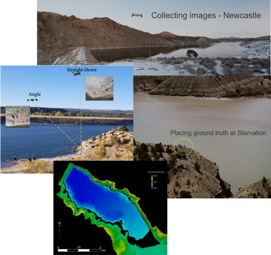
• sUAVs can easily access remote shoreline areas—for the Starvation reservoir survey presented here, we flew the sUAVs from a boat;
• sUAVs are easily deployed; this can allow data to be taken at low pool to overlap with sonar data or coincide with sonar data to minimize crew mobilization;
• Surveys are easily completed with minimal time and expenses compared to traditional methods; they can be performed repeatedly and often, which means they can be used to help track sedimentation or other reservoir processes.

A challenge of using sUAVs in conjunction with sonar surveys to develop full-pool bathymetric maps has been developing useful methods that provide the needed accuracy that can be efficiently implemented for surveys that can cover kilometers of shoreline and require computation of long, thin topographic models. Until recently, images collected from sUAV platforms were not useful for photogrammetry because the position of the camera was not known to provide sufficient accuracy and the cameras used were not of high enough quality. New computation algorithms address both of these issues by using a large number of images combined with minimal ground truth data to generate accurate terrain models [4,5,6,7]. For example, Ruberti et al. [8] used sUAV imagery to assess sea cliff stability, addressing challenges similar to those encountered when developing full-pool bathymetric maps, and there have been many other studies that used sUAV imagery to generate terrain models, though in different application areas without the issue related to long, thin models [9,10,11,12,13,14].

We present a method to use sUAVs to develop terrain data for full-pool bathymetric maps. We present both the methods and the unique challenges associated with modeling thin strips of shoreline over long distances as most terrain models are not long and thin and do not have water in the majority of the images. We present these methods to help researchers and practitioners more effectively use these new tools and methods.

Researchers and practitioners have used imagery from sUAVs and Structure from Motion (SfM) algorithms to generate accurate topographical models [15,16]. This is a more cost-effective method for generating topography for small areas compared to traditional aerial photogrammetric methods. Extending these general terrain models, recent studies have demonstrated the use of sUAVs and SfM technology in many environmental resource fields, including the field of water resources [15,17,18,19,20,21,22,23,24], and other applications [25,26]. The majority of this work revolves around using sUAVs’ data collection methods to create accurate three-dimensional (3D) topographic models. For example, researchers have monitored braided river channels using photogrammetry [21], and sUAV images have been used to generate detailed ortho-images of river streambeds and process these images to accurately estimate the particle size distribution of streambed sediments and erosion processes [22,27,28,29,30]. LiDAR has been used in conjunction with sUAV technology to create topo-bathymetric models [31]. LiDAR is a tool that could be used in place of SfM photogrammetry to model shorelines, although LiDAR surveys tend to cost more as they generally require larger UAVs and more costly sensors. SfM-based photogrammetry has been used to supplement standard sonar collections by collecting data at shallow depths that sonar technology cannot accurately model [17]; our method extends this research to above-water areas. Others have used sUAV-based methods to monitor changes in coastline due to wave run up [18] and evaluate water resource infrastructures such as spillways [15]. Similar to this study, other studies have also evaluated various parameters on procedures and their effect on accuracy including altitude, ground control, camera angle, and others [5,32,33,34,35,36]. This is not an exhaustive review, and many more examples of using sUAV data and SfM algorithms to generate terrain data and to explore the impact of various parameters and processes exist. This manuscript identifies and discusses challenges specific to using sUAV data with SfM algorithms to generate terrain maps of reservoir shoreline areas and integrate these data with sonar data of the below-water portion of the reservoir.

Most UAV-based surveys use a pre-determined grid format for flight patterns over areas where the width and length are of similar magnitude; thus, most of the current literature on GCP spacing discuss and address a grid format for flight patterns and GPC placement [34,36,37]. Although gridded flights are most common for collecting over typical sites, some jobs require long, thin models such as the shoreline surveys (discussed in this paper), roads, road cut slopes, levees, or canals [33]. The issue of GCP spacing and orientation along long, thin corridors has been the subject of some research which explored the expected accuracy with different GCP spacing and orientation along a relatively long stretch of road [5]. This work is similar to that presented here, but roads generally follow regular lines, without significant changes, which is different than a reservoir shoreline which has a more fractal geometry. Shorelines also pose an issue during fieldwork as placing many GCPs may be unrealistic, time consuming, or costly as parts of the shoreline are often relatively inaccessible for ground-based transportation.

Post-construction, full-pool bathymetric maps are an important tool for properly managing and maintaining reservoirs. Full-pool bathymetric maps can help assess risk by providing data for inundation modeling and to produce storage capacity curves to manage reservoir storage and drawdown. If maps are updated regularly, the resulting storage capacity curves can be used to predict the estimated lifetime of a reservoir due to sedimentation. With a time-series of bathymetric maps, data on sediment flow and reservoir filling can be computed. Managers can use information to understand the magnitude, trend, and impact of sedimentation.

As noted, a post-construction, full-pool bathymetric map extends from the highest point of a dam or spillway crest to the lowest point of the reservoir. Areas above the normal water line are important as shoreline terrain, especially in inlet delta regions, changes over time as water level changes, causing erosion and deposition in the region above the low water level. Extending these maps to the spill or dam crest allows users to better manage reservoir filling and evaluate the risk of dam over-topping during high flows, such as those that occur during spring runoff, though the region above the average high water mark experiences less change. For older reservoirs, this may not be true, as erosion, construction, and other activities can significantly change the area between the average water levels and the spill or dam crest.

Historically, bathymetric maps were produced by interpolating between points measured at a relatively large spacing throughout a reservoir, typically on the order of a few, up to 10, meters or larger depending on the size of the reservoir. These measurements were made using traditional survey methods before the reservoir was filled, or using single-beam sonar surveys after filling. More recently, as equipment costs have fallen, methods to accurately collect data using multi-beam sonar to collect data below the water surface have been established. Multi-beam sonar surveys produce a dense point cloud that represents the reservoir bed. Multi-beam sonar produces measurements with a spacing of approximately a few centimeters at typical reservoir depths.

One issue associated with generating post-construction full-pool bathymetric maps is that sonar cannot collect data above the water surface. In addition, it is difficult, because of access issues, for sonar surveys to collect data in shallow areas or the shallow flood plains in a reservoir. The only way to access these areas is to survey the reservoir during full-pool conditions when these areas have deeper water, and in many cases, the water in these areas may not be deep enough for a sonar survey. However, the areas that are too shallow for sonar are often exposed at low pool. The use of sUAV to acquire imagery of these areas during drawdown conditions allows data collection in these shallow areas and also in areas that are rarely inundated above the normal high water mark, as reservoirs are generally not filled to spill conditions.

The use of photogrammetric methods to produce topographic maps is well established, especially for pre-construction surveys. We have not found any reports and assume that it has not used to generate topographic maps of shallow and shoreline areas in bathymetry studies. We believe this is because the area above the water line is long and narrow; for these uses, traditional aerial photographic methods, while useful, are not the most efficient methods for collection.

Erena, Atenza, García-Galiano, Domínguez, and Bernabé [19] reported using sUAV technology for topo-bathymetric monitoring of reservoirs. They used sUAVs to capture topography near a dam and then integrated these topographic data with sonar data, but it is unclear if they integrated photogrammetry-based shoreline modeling for the entire shoreline of the reservoirs or if they only used sUAV-based photogrammetry to more accurately model the area near dams. Their paper implies that LiDAR data from a regional survey were used to model the shoreline areas of the reservoir away from the dam, rather than data from sUAV images. Similar research has been done modeling shorelines using a fixed-wing sUAV to collect data over shallow lake and coastal shorelines [23,24]. A fixed-wing sUAV typically collects nadir photos, which is not optimal for steep shorelines or shorelines with sheer cliffs.

Our work extends these approaches by evaluating and recommending a method to provide a post-construction full-pool bathymetric model using only multi-beam sonar and sUAV data, including recommendations on image collection, ground truth placement, and data integration. Our method addresses the challenges associated with developing models on long, thin regions with steep slopes. We use sUAV-captured imagery to compute a topographic model of the shoreline of a reservoir and integrate those data with sonar data to create full-pool bathymetric maps of reservoirs. We identify potential issues associated with developing bathymetric maps that use these long, thin terrain models and that have water in the majority of the images used for model creation. Published studies only minimally address developing long, thin models or using images with extensive water or sky in the image. One driver for this study is that access to shoreline areas is difficult and time-consuming, which affects the efficiency of placing ground truth. We present challenges and methods for integrating digital terrain models from two different sensor platforms, multi-beam sonar and sUAV images, a challenge nearly unique to bathymetric mapping.

Through this effort, we hope to give researchers and practitioners the knowledge and assurance to use these new tools to develop data to better understand reservoir processes and assist reservoir management. This study reports on the creation of post-construction, full-pool bathymetry maps for two reservoirs. These two field studies represent significant collection efforts and, as a result, highlight issues that may not be apparent in smaller comparative studies or in the more controlled studies required for algorithm development. Our study is neither a comparative study nor a controlled study for algorithm development. Instead, this is a case study approach where we identify and address challenges and solutions for a real-world problem, specifically issues encountered in full-scale fieldwork. We show that this application, creating post-construction, full-pool bathymetric maps, can be solved using software and surveying techniques that are widely available to agencies and others that manage reservoirs.

2. Materials and Methods

2.1. Background

Multi-beam sonar data and SfM algorithms using sUAV imagery both generate 3D point clouds which represent the ground surface below and above the water line, respectively. Figure 1 outlines our method that creates SfM point cloud data, then integrates those data with a sonar point cloud to create a reservoir full-pool topographic model. As part of the study, we first describe and present the process we used to create the full-pool bathymetric maps.

2.2. Process Description

2.2.1. Experimental Overview

We performed five different investigations to determine how various parameters and procedures affected model creation and data integration. For all the models, we followed the methods presented in Section 2 for both model creation and model comparison. The areas we investigated and present here are:

• Ground control point (GCP) spacing;
• Effects of masking water;
• Effects of using no ground control points;
• Effects of an incorrectly tagged ground control point;
• Method for integrating sonar and sUAV data.

We used the Starvation Reservoir study site (Figure 2) to explore GCP spacing. We performed investigations 2–5 at Newcastle Reservoir (Figure 3). For investigations 2–4, we used an experimental site located on the dam of Newcastle; for investigation 5, data integration, we used the entire reservoir. We used Newcastle Dam for investigations 2–5 because of its easy access and smaller size. This resulted in significantly fewer images required for model creation and allowed for more rapid turnaround. Because of the relatively small size of the dam, only one GCP was used in the middle of the dam for these experiments. The experimental site located at the dam was a relatively small (0.4 km) area that included the data in the northwest corner of Newcastle Reservoir.

2.2.2. Image Collection and GCP Establishment

At Starvation Reservoir, we used two Parrot Anafi sUAVs equipped with the standard camera to collect images. We took photographs in nadir view (directly above the shoreline) as well as from an oblique view (camera was angled towards the shoreline). We used the oblique view to capture images approximately normal to the ground slope. For many of the shoreline regions, the shore rose steeply, so it required a combination of nadir and oblique images to capture the terrain. The overlap between photos was relatively consistent because we flew the Anafi sUAV manually along the shore and automatically acquired photos at 10-m (30-ft) intervals, which resulted in an overlap between photos of at least 70%. We flew at an above ground level elevation (AGL) between 50 (150 ft) and 75 m (200 ft), for the nadir and oblique acquisitions, respectively.

At Newcastle Reservoir, we used a DJI Phantom 4 quadcopter equipped with the integrated camera for image collection. We collected images in both nadir view (directly above the shoreline) and oblique view approximately normal to the steep shoreline. The overlap between photos was not consistent because we flew the sUAV manually and the photos were automatically taken at 5-s intervals, resulting in variable spacing. We estimated that the overlap between photos was at least 70%. We also flew the floodplain near the inlet to the reservoir. Since this area was not a narrow strip, we used a pre-programmed automated flight path with image acquisition to guarantee that the images had at least a 70% overlap.

GCPs consisted of painted cross targets approximately 0.5 m squared. We staked the targets to the ground using large steel pegs, then we measured and established the center of the target using a TOPCON HIPER VR GTK GPS system. We established a base station at a known point and then connected a rover GPS antenna to the base station for real-time kinematic (RTK) corrections; we then performed a minimum of a 30-s measurement on each target. These procedures should result in sub-cm accuracy for the GCP coordinates. We used the WGS84 projection and UTM Zone 12N Coordinate System. We placed 34 GCPs at Starvation Reservoir, with an average spacing of about 1.5 km (1-mile), and 8 GCPs at the Newcastle site with a spacing of less than 0.8 km (0.5 miles).

For each reservoir, we created a file with a list of the GCPs and their coordinates. This file was later uploaded to the processing software and then each target was identified in the image in which it occurred and was associated with the correct coordinates.

2.2.3. Model Creation using SfM

We created shoreline models for the five investigations using the commercial SfM software package, Agisoft Metashape (Version 1.6.1.10009).

After reviewing the images and removing those visually not suitable for model creation, we followed the following steps to create the model:

• Import photos and GCPs into the photogrammetry software;
• Mask the water in the nadir images;
• Mask distance areas and sky in the oblique images;
• Identify and tag GCPs in photos;
• Use the software to compute an optimized camera alignment—this creates a sparse point cloud georeferenced by the GCPs;
• Compute a dense point cloud from the sparse point cloud.

Steps 1–4 require user interaction; the software executes steps 5 and 6. The Starvation model took approximately 60 h to set up and processing the 5193 images (steps 5 and 6) took approximately 13 h. The Newcastle model took approximately 20 h to set up and processing the 1627 images took approximately 9 h.

2.2.4. Sonar Data Collection and Model Creation

We conducted the sonar data collection surveys from a pontoon boat using an Imagenex DT 101xi, which is a multi-beam echo sounder with an integrated motion reference unit and a sound velocity sensor that measures temperature and sound velocity near the sonar transducer head. The motion reference unit has a pitch and roll accuracy of 0.04 degrees and a heave accuracy of 5 cm or 5%, whichever is greater. The DT101xi has 480 beams with an approximate 120-degree beam width. We used a survey speed of not more than 8 knots, which resulted in a nominal measurement spacing of less than 5 cm between points in either the longitudinal or transverse directions, though data at the ends of the beams are wider spaced.

We used the Imagenex DT100 SIR (Sensor Interface Relay) power supply/timing box to control the DT 101xi sonar unit. We connected the DT100 to a Global Navigation Satellite System/GPS (GNSS/GPS) receiver mounted vertically 1.5 m over the sonar head. We used a Hemisphere Vector V103 Smart Antenna to record the GPS location during the sonar survey. Gyro and tilt sensors are integrated into its design to improve system performance and provide backup heading information in the event that a GNSS heading is not available. GPS sensors are located approximately 2 ft apart and mounted internally on opposite ends of the antenna. To measure sound velocity profiles, we used a CastAway-CTD probe with a built-in GPS receiver. The CastAway-CTD measures conductivity, depth, salinity, and temperature and records density and sound velocity. We used these measurements to calibrate sonar data.

We managed data collection, processing, and storage using HYPACK software (xylem HYPACK 2020). We recorded the raw sonar data using HYPACK software that we also used to plan and execute the data collection, including survey tracks and real-time data collection monitoring to verify the targeted 50% overlap on each track. We used HYPACK SWEEP (xylem HYPACK SWEEP 2020) to process the raw sonar data to generate the final point cloud.

In general, we followed US Bureau of Reclamation sonar survey methods. The sonar was bow-mounted on our pontoon boat and removed from the boat each day. We performed patch tests at the beginning of each survey, though they are only recommended when you reconfigure a boat. Patch tests adjust for issues with the boat and survey head not being level. We took sound velocity profiles a minimum of three times a day—morning, noon, and at completion. We took additional sound velocity profiles when reservoir conditions changed, such as near an inlet, outlet, or in other conditions that could affect temperature profiles. We used HYPACK software to process the raw sonar data and apply corrections. We maintained an approximately 50% overlap in sonar swaths, meaning that most locations were collected near the center of the sonar swath after processing; this reduced the impact of data near the ends of the beam width having a larger spacing. We used HYPACK software to process the resulting corrected data to create a point cloud of the reservoir bed.

2.2.5. Computing Accuracy Differences between Point Cloud Models

Determining the accuracy of point clouds is difficult [38]. Methods to evaluate traditional survey accuracy relied on instrument and method calibration, which is not applicable to the practice of using un-calibrated cameras on unstable unmanned aerial System (UAS) platforms [38]. The most defensible method to compute the accuracy of a point cloud is to use a dense network of ground truth that is not used in model creation [38,39]. There has been some work on establishing the accuracy of LiDAR-generated point clouds, though Toth, Jozkow, and Grejner-Brzezinska [38] note that with the exception of the Vertical Accuracy Reporting for LiDAR Data (VARLD) guidelines, that there are no generally accepted methods for point cloud accuracy—which, for the surveying methods reported here, is the final product. Kim, Park, Danielson, Irwin, Stensaas, Stoker, and Nimetz [40] state that one method to assess LiDAR accuracy is to compute the error of the vertical component and that assessment of point clouds in full 3D (three dimension) is not routinely performed. Work is continuing on this topic, such as using geometric extensions of man-made structures [41] with new standards being developed [42]. These approaches are not tractable for our work since we did not have a dense network of ground truth or geometric structures (e.g., building roofs) that could be used to identify common points for accuracy assessment.

To assess the accuracy of our models, we assumed that the model with the most ground truth was the most accurate, and then, we used the cloud-to-cloud comparison (CCC) tool in CloudCompare software (version 2.11). The CCC tool calculates the Euclidean distance from one point to the nearest neighbor of that point in the other point cloud. This is done for each point in the point clouds and computes the root mean squared error of the distance between the two point clouds in 3D space [40,41]. We used this average distance between the point clouds to quantify the effects of the different investigations we performed. We used the point cloud created with the densest ground truth and best prepared images (water and sky masks) as the reference cloud for comparison with the other clouds.

We produced point clouds with ~2.7 billion and ~272 million points for Starvation and Newcastle reservoirs, respectively. These point clouds represented the shoreline for the entire reservoir and we used all the available GCPs for computation. For specific tests, we created models of smaller test areas at each reservoir, as described in Section 3.

We present the error between the clouds in several ways; after using the CCC tool to compute the Euclidean distance between each point, we calculated average and standard deviation for the difference between the two clouds, and we also analyzed the distributions of these differences. To evaluate spatial issues, we computed a new point cloud colored by the distance between points at each location. This allowed us to evaluate how the topography and other spatial issues affected the accuracy of the models.

2.2.6. Knitting SfM and Sonar Models

We used the HYPACK software to knit the points clouds from the sUAVs and the sonar into a single dataset. Prior to merging, we removed any outliners from the datasets. This was done in two passes. HYPACK identifies points that are statistical outliers in a small region—we selected 2.5 standard deviations as the anomaly threshold for a 1-m region—and we also visually evaluated the point clouds to identify and remove anomalous points. After cleaning the point clouds, we resampled both point clouds to a 1.5-m (5-ft) grid spacing.

For both reservoirs, sUAV data were collected either coincidentally or slightly prior to sonar data collections. This meant that the two datasets did not overlap, and there was a small gap in most shoreline areas between the highest sonar data and the lowest sUAV data. For the final integrated dataset, this was addressed by using a spatial interpolation routine to interpolate the data between the two datasets.

One challenge in merging the point clouds is that the sonar data were not accurately georeferenced to a global coordinate system, though they are internally consistent. For the integrated dataset, we used the sUAV data as the anchor and translated the sonar data to match. There was no need to rotate the data. We did use GPS receivers to acquire the sonar data, but these GPS coordinates were not corrected for GPS drift, which can be up to 10 m. We generated the sUAV data using GCPs’ coordinates, and assigned pixels were geolocated to within approximately 3 cm horizontally, the approximate resolution of the images.

To merge the two point clouds, we created transects of both the sonar and sUAV point clouds at several locations along the shore line. For surveys with overlapping points, i.e., where sonar data were taken at high pool and sUAV data at low pool, the two datasets could be easily merged by visually aligning the two datasets. For our datasets, we visually matched the slope of the surface to align the two datasets. After alignment, we used the inverse distance squared interpolation method to fill the gaps between the two datasets and resample the datasets to a common 1.5-m grid. Results are discussed later.

2.3. Case Study Locations: Starvation and Newcastle Reservoirs

2.3.1. Case Study Background

We present and discuss our method to develop full-pool bathymetric maps using a case study approach with two reservoirs, Starvation and Newcastle, located in the State of Utah in the western United States, which has a semi-arid climate. Starvation is a large reservoir with an irregular shoreline (Figure 2). Newcastle is a smaller reservoir with a more regular shoreline (Figure 3). The Starvation shoreline is such that the ratio of shoreline length to reservoir area is significantly higher than that of Newcastle, as shown in Figure 2 and Figure 3.

In this section, we discuss the issues associated with various steps in generating a post-construction, full-pool bathymetric map and, where applicable, we present methods, such as guidelines for ground truth spacing, that make the process more efficient. We discuss the impacts these methods have on the accuracy of the resulting topographic model. The two reservoirs have different characteristics that we use to highlight issues associated with our method. The majority of the work was done at Newcastle Reservoir because of the reservoir’s small size, which made it more tractable both for field work and computer processing. We evaluated GCP spacing at Starvation Reservoir as GCP spacing on this large reservoir had a significant impact on the amount of time required to complete the survey.

Managers for both reservoirs expressed a need for updated and future periodic bathymetric surveys, mostly to address expected large sediment loads. There have been large recent wildfires in the reservoir watersheds and these fires are projected to significantly increase the near-future sediment loads. By establishing a baseline and periodically resurveying, these loads can be quantified. We expect most of the sediment to be deposited during full-pool conditions during spring runoff. This means it may be possible to perform updates using only sUAV data collected at low pool when these sediment deltas are exposed in the late summer or early fall. Collecting data with sUAVs would allow updated maps to be generated with minimal effort—a few hours for GCP placement and less than an hour of flight time.

These reservoirs are primarily used and managed for irrigation storage, which means that typically, they are filled in the spring after snow-melt and reach low-pool status in late summer or early fall. The semi-arid climate means that little vegetation is present on reservoir shorelines in the region above normal high water levels and below full pool. There is little aquatic vegetation, so the region between normal high water and low pool, is essentially sediment or rock; this region is annually exposed during drawdown. The lack of vegetation is optimal for sUAV imagery as SfM algorithms cannot easily separate the ground surface from the apparent ground surface created from the tops of vegetation.

2.3.2. Starvation Reservoir

Starvation (Figure 2) is a relatively large reservoir over 9 km (6 miles) in length with several bays and arms that significantly increase the shoreline area. The Starvation Reservoir shoreline has some flatter areas near the north end of the reservoir, but the majority of the reservoir has steep banks or cliffs. This made access difficult to the area for the sUAV survey and made placing GCPs for the aerial images challenging and time consuming. We used Starvation Reservoir to quantify the impacts of different GCP spacing along the shoreline.

We placed 34 GCPs around the reservoir, with an average spacing of about 1.5 km (1 mile). On the north shore of the reservoir, in the test strip, which is shown by the yellow box in Figure 2, we placed GCPs much closer for the GCP spacing investigation. GCP placement took approximately 10 days. Because the shoreline is essentially inaccessible from the ground, we used a boat to ferry crews to the GCP locations along the shoreline. We collected approximately 6000 images for model creation. We used 86.7% of the collected images after removing images that were not suitable for processing. It took approximately 3 days to fly across the reservoir. To collect images, we flew two sUAVs simultaneously to take both nadir and oblique images. The sonar survey took approximately 15 days to complete.

2.3.3. Newcastle Reservoir

Newcastle Reservoir (Figure 3) is a relatively small reservoir, less than 1.6 km (1 mile) in length and approximately 0.5 km (1/3 mile) in width. It is shaped like an ellipsoid, with minimal shoreline for its area.

The eight GCPs at the Newcastle site are shown in Figure 4. Since the shoreline was easily accessible, the GCPs were spaced less than 0.8 km (0.5 miles) apart. At Newcastle Reservoir, we collected approximately 1765 images. Of these images, we used 92.2% after removing images that were not suitable for processing. GCP placement took approximately 6 h. Image collection took approximately 2 h. We only flew one sUAV at Newcastle, as opposed to two at Starvation. The sonar survey took approximately one day to complete. We used Newcastle data to complete the majority of the investigations, with most of the investigations using data from the dam, shown in the yellow box in Figure 3.

3. Results

3.1. Experimental Overview

In this section, we present the results from the five investigations. We performed the first investigation, GCP spacing, at Starvation Reservoir; we performed investigations into the impacts of water/sky masking, no GCPs, and incorrectly tagged GCPs using Newcastle data. At both reservoirs, we merged the sonar and sUAV datasets and used those data to discuss issues associated with dataset merging.

3.2. Ground Control Point Spacing Experiment

GCP placement requires significant time and effort when performing an sUAV survey. For example, at Starvation Reservoir, because of the inaccessible nature of the shoreline, it took approximately 10x as much time to place the GCPs as it did to capture the drone images as Starvation Reservoir has a total perimeter of approximately 43.5 km (27 miles). As noted, GCP placement at Starvation Reservoir took about 10 days, using an average spacing of 1.6 km (1 mile). Travel time to Starvation Reservoir from campus is approximately 2 h, so the first and last days of the two-week period when we placed ground truth were quite short as they included travel time and the time required to ready and launch the boat. We estimate that to place GCPs at a 0.4-km (1/4-mile) spacing, it would have taken approximately 20–30 days; it is not a factor of four because survey teams would have been able to walk between some of the GCP locations. Starvation Reservoir provides a good demonstration of the efficiency that can be gained by minimizing the number of GCPs used.

Typical bathymetric maps are generated with either 1- or 1.5-m contours based on the United States Army Corps of Engineers guidelines. The models we generated, based on sUAV flights at approximately 30 m (100 feet) AGL, resulted in point cloud models with resolutions of a few centimeters, with accuracy affected by a number of parameters as discussed in the remaining sections, but most importantly the use of GCPs. We wanted to determine a maximum GCP spacing (i.e., the minimum number of GCPs) that would support a model with a resolution sufficient to create a usable bathymetric map, based on the assumption of 1-m contours.

We established the Starvation Reservoir test site at the northern portion of the reservoir, shown as the yellow box in Figure 2, with more detail and the locations of the GCPs in Figure 5. The test site consists of a 3.2-km (2-mile) stretch of the reservoir with an irregular shoreline that includes several small inlets or bays, areas with flat banks, and areas with steep, almost vertical, banks. At the test site, we placed GCPs at an approximate 0.4-km (quarter-mile) spacing. For this test strip which had good access, meaning that the GCP-placement teams could walk between the GCP locations, placement took approximately 4 h. In contrast, image acquisition took significantly less than one hour and much of that time was spent preparing equipment before and after the flight, tasks that need only be done once. The actual flight time was approximately 20 min and could have been completed faster.

For this investigation, we first created a reference model using all of the GCPs. We then created models using sub-sets of different spacings of the GCPs to determine the impact spacing has on model creation for bathymetry mapping.

We visually evaluated the model generated using the 0.4-km (0.25-mile) spacing and did not identify any anomalies—because of the method in which the models are generated, they exactly match the terrain at the GCP locations, and the GCP points cannot be used to compute error measurements. While there is significant elevation change away from the reservoir shoreline, by definition, the elevation at the water edge is constant and does not change; this provides an excellent point for evaluation. The reference model met these criteria. While it is difficult to see in a two-dimensional image, the model represents 3D data with a flat shoreline with steep banks rising from the reservoir. The bay in the upper left part of the image is relatively flat away from the shore, while the area in the far right consists of a very steep, almost cliff-like bank.

To determine the maximum spacing that would result in an acceptable model, we created models using GCP points with 0.8-km and 1.6-km (½- and 1-mile) spacings; Figure 6 panels (a) and (b) show the resulting models, respectively.

We used CCC, as described in Section 2.2.5, to compute the distance between the different point clouds. Figure 7 panel (a) presents the difference between the model generated with 0.8-km (½ mile) GCP spacing with the reference model. This figure is colored by the distance or difference between the two models at each point. The difference, mostly in the vertical direction, is shown as color, with the color scale indicating the magnitude of the difference. We found the average error between the 0.8 km (1/2 mile) model and the reference model to be 4.5 cm. The top panel of Figure 6 and Figure 7 shows that the portion of the model with the largest error is in the eastern part of the test site. In this region, the area imaged by the drone extends a significant distance past the last GCP, well above the reservoir elevation, and this region has very steep, almost vertical banks. The areas with the highest error are significantly higher in elevation than the reservoir shoreline and the locations of the GCPs and would not be used in generating the bathymetric maps as they are above the spill level of the reservoir. Previous work, not reported here, showed that models generated using these algorithms do not extrapolate past the GCPs accurately. For accurate model generation, GCPs should be placed near the edges of the areas of interest. The top panel of Figure 7 clearly demonstrates this issue with the area of highest error extrapolated both horizontally and vertically past the extent of the GCPs.

The bottom panel (b) of Figure 7 compares the model generated using 1.6-km (1-mile) GCP spacing with the reference model. We found that the average error between these two models was 5.5 cm. We limited the 1.6 km (1 mile) model to a narrow band along the shoreline, more consistent with the high water mark and spill elevation for the reservoir. This means that the 1.6 km model did not include the area beyond the GCPs that resulted in the highest error for the 0.8 km (½ mile) model. Figure 7 panel (b) shows that areas with larger errors were more interspersed throughout the spatial area, with the largest errors in the region in the southwest. In this area, colored red in panel (b), the bank rises very steeply, almost a vertical cliff. Thus, very small errors in position can result in very large vertical errors, while not significantly affecting bathymetry contour generation. In addition, because of shoreline access, it was difficult to place GCPs in these cliff-like areas, the spacing between the last two GCPs was more than a mile. This area went from a very narrow shore with steep banks near the middle GCP, to a flat inlet area in the northwest portion of the model, to a steep bank without a flat shore near the GCP in the southwest corner. This is a very large change in terrain, and even under those circumstances, the model generated using GCPs with 1.6-km spacing only had an average difference of 5.5 cm from the model generated with a 0.4-km GCP spacing.

3.3. Effects of Water Masking

Most SfM software includes a tool to mask out and omit parts of photos from the algorithms that compute the sparse cloud alignment. These algorithms rely on image analysis routines that match locations in the overlapped images and use these match points to compute both the camera and ground locations. Water can be problematic for SfM because it either lacks distinct features or has transient features (e.g., waves and ripples) which change between images. Both of these hinder the image-matching algorithms responsible for point cloud generation and also hinder automated methods for rejecting poorly matching points. Most algorithms have methods to reject matching points whose alignments significantly different from the average; however, if the images contain portions that are water, a large portion of the matches are incorrect and invalidate the statistics used to reject incorrect matches. The alternative is to manually mask out water areas, which can be time consuming.

Portions of the images we acquired of the shoreline all contained water, some to a very significant extent. Many of the oblique images contained portions that were distant from the modeled area and many also included sky. These regions cause issues with the automated point matching, similar to water regions. To create accurate models, these image regions (i.e., water, sky, and distant areas) needed to be marked and masked so that the processing algorithms ignore them. The commercial software we used required this to be done by hand, which is common for all the commercial software packages with which we are familiar. Our use case, modeling a reservoir shoreline, is not common, and unique issues are not likely to be supported by commercial packages.

Because water masking requires opening and masking each image, this can be very time consuming. The Starvation Reservoir model included over 6000 images and the much smaller Newcastle model included nearly 2000 images. Even if images could be processed in approximately 10 s (most took longer), the Newcastle images would require nearly 16 h of editing. We designed this experiment to determine the accuracy impact of masking the images and whether this step is required. The algorithms implemented by the commercial software reject anomalous matching points and, in general, handle images that contain distance objects well. However, water in the images and, to some extent, sky generate faux match points in significant numbers, causing the automated point rejection based on statistics to fail.

We used the Newcastle Dam site, the region shown in yellow in Figure 3, to perform this investigation. This area is relatively small and includes the dam, which has more regular geometry than most shoreline areas.

Figure 8 shows match points identified by the algorithms which are incorrect as they are in the water. Water does not have stable, stationary features but does have features that appear to be matches when they are not. We identified any match points in the water likely an error, so some may be legitimate if they are on submerged but visible features. Figure 8 shows that for this region, a large number of these points might be in this category as the points are in shallow water near the shore, and when visually reviewing the images, we can see submerged features. While these objects are stationary and legitimate match points between the images, because the objects are underwater, diffraction effects cause the object to appear in different locations depending on viewing angle and these points cannot be used for model generation as they distort the geometry.

If erroneous tie points are used in computing geometry, the algorithms try to minimize the difference in the assigned elevation and location of each tie point among the images, generally accepting some minimum or average value, meaning both the near-onshore points and the points in the water are incorrect. This results in inaccurate models, with the most obvious errors being areas where points representing the water are projected above or below the water surface.

For this investigation, we generated a reference model using images where we masked the water. We then compared this reference model to a model generated using images without masking. Figure 9 shows the difference between these two models with the largest errors or differences in the shoreline region, close to the water, and the water itself, as would be expected. The difference between these two models was significant, with errors in the near-shore area of over 20 m. The average difference between the two models was 0.2 m, but this includes large shore areas not affected by the water. The right side of Figure 9 shows a histogram of the error, which is a right-skewed distribution with a maximum difference of 24 m, but the majority of the errors were in the smallest bin; spatially, Figure 9 shows that this error is highest in the areas near the water–shore interface.

Figure 9 shows that while there are substantial errors introduced by including water in the images, these errors, for the most part, are limited to the very-near on-shore or off-shore portions of the model, while more minor errors are introduced near the edges of the model, away from any GCP point influence. Manual image masking is very labor-intensive, and the limited spatial distribution of these errors might lend itself to other methods. We recommend that methods should be evaluated that automate or semi-automate water detection and masking in the images as the best path forward. There are algorithms to identify water and sky in images, though they are not integrated into commercial packages. The current algorithms can mostly identify and address image areas that contain distant objects in the oblique images.

3.4. Effects of no Ground Control Points

We used the Newcastle Dam site to test the nature and magnitude of the error introduced to the point cloud model when generating a model not using any GCPs. This is a somewhat limited investigation as the area we evaluated is small. We expect these results to scale, though trends can be introduced to large models where errors increase with the model size, though local, smaller regions have errors similar to those presented here.

We created a reference model using the GCP in the middle of the Newcastle Dam experimental site and compared that to a model created without using a GCP. The sUAVs used in these experiments capture GPS coordinates of the location of the camera when an image is taken. The main unknown parameter computed by the SfM algorithms is the location of the camera, so this information is used to build a model. However, these GPS receivers are not survey-grade and can have errors in location in the order of a few meters with an sUAV. In addition, common sUAVs include less accurate inertial measurement units (IMUs) which measure the airframe attitude (pitch, yaw, and roll), which affects model accuracy. If an sUAV is equipped with a real-time kinematic (RTK) GPS system and high-precision IMUs to accurately measure the location and attitude of the camera to within a few centimeters, accurate models can be generated without ground truth [43,44,45,46,47]. However, sUAVs with these sensors are less common and relatively expensive.

Model generation without GCPs depends on the accuracy of the sUAV’s GPS and IMUs. For this investigation, we collected data with the very commonly used DJI Phantom 4 sUAV. This drone is relatively inexpensive and is used by many researchers and practitioners. We expect that our general results can be extended to other similar drones without RTK GPS or high-precision IMUs; the actual values may be different for different systems.

Figure 10 shows the difference between the reference model and the model generated without GCPs. What is readily apparent in the image is that the model generated without GCPs is relatively self-consistent but not well located in absolute reference space. The difference between the two models is similar to the reported accuracy of standard GPS signals, or about 10 m. The right side of Figure 10 shows that the average Euclidian distance to the nearest neighbor between the reference point cloud and the point cloud without GCPs was 10.7 m, with an error distribution that is approximately normal with an average difference of 10.7 m and a standard deviation of 1.5 m. This error is the largest of any of the experiments we performed.

Since the model generated with no GCPs is self-consistent, we could translate the model and obtain a close match to the reference model. In practice, this is done using a GCP point that may be identified or measured after data collection. For longer collections using multiple flights, a single correction would be problematic as the GPS signal “wanders” significantly. We expect that images collected over a day or several days would not be as self-consistent. GCPs provide a common point of reference for these longer collections.

3.5. Effects of an Incorrectly Tagged Ground Control Point

One common error in photogrammetry is to mis-tag ground control. This mistake is due to user error either in the tagging process or in collecting and recording the field information. We designed this investigation to evaluate the impact of mis-tagging GCPs. This causes two general issues: the global reference frame for the data is incorrect, and the on-board GPS measurements from the sUAV appear to have a larger error. This can also cause problems as portions of the model are referenced to different locations, requiring the algorithms to minimize and distribute the error while honoring the GCP points.

We used the Newcastle Dam site to evaluate the nature and magnitude of the error introduced to the point cloud model due to mis-tagging GCPs. The reference point cloud had only one GCP in the middle of the dam. This is near a “worst case” scenario, where there is only a minimal GCP and that is in error. The GCP appeared in seven images; we only mis-tagged it in one, and we mis-tagged the GCP in one photo by approximately 2 m.

Tagging GCPs consists of locating GCPs, previously surveyed and marked in the field, in images and assigning them a known location in each image in which they occur. There are some automated routines for this task if the GCPs have special patterns. In most collections, GCPs will appear in at least two images, and often three or even four depending on the location of the GCP and the overlap scheme of the images. Errors can occur by misidentifying locations in the images, clicking near—but not on—a GCP in an image (often caused by users “zooming out” to tag GCPs quickly but reducing the apparent resolution of the image) or due to recording or transcription errors in the location information. There can also be cases where the location of a GCP is in error—we did not investigate this issue.

Figure 11 shows the difference between the reference model and the model with an incorrectly tagged GCP. Figure 11 shows that this produced a unique error pattern where there were parallel planes across almost the entire model. This location showed that there was a difference between the reference and experimental models of between a meter and three meters in the z-direction, but both models were aligned in x-y (horizontal) space. We found that the average Euclidian distance was 0.29 m, with a standard deviation of 0.9 m. The right side of Figure 11 shows that the log error distribution, i.e., we log transformed the errors before generating the histogram. A log transformation was taken because the original error distribution was extremely right-skewed.

3.6. Knitting of Sonar and sUAV Data

We used the reference model, generated from sUAV images, of Newcastle and the data collected by our multi-beam sonar to develop a method to merge the two datasets. The sonar data were collected with survey-grade GPS receivers but not corrected using RTK or post-processing kinematic (PPK) methods, so while the data were self-consistent, they were not well located in absolute space.

We developed a method to use cross-sections of both sonar and sUAV models to georeference the sonar cloud using the sUAV data and to merge the two datasets to produce a final model or point cloud. These data can then be used to create a contour map or digital terrain map to generate bathymetry data, such as storage/elevation curves, for the reservoir.

Figure 12 demonstrates how we used transects and cross-sections of the two models to properly orient the sonar model in space. We created several transects, normalized to the shore line in horizontal space. We placed these transects in regions where we assumed that the slope of the ground is more or less constant, with no large changes—areas such as dam faces, sediment regions, or flat areas, not areas such as rocky shorelines or cliffs.

The left side of Figure 12 shows one transect located on the dam face; the other transects are not shown. The right side of Figure 12 shows a line which represents the extended ground slope of the two datasets; the sonar data were translated until these slopes visually had a good match. This was done for all transects, and continued manually until a good match was apparent. We evaluated matches visually.

For the Newcastle Reservoir collection, the initial two models did not overlap as the sonar and sUAV data were collected on the same day and sonar cannot collect up to the water elevation. This resulted in a gap between the sonar data and the sUAV data, which can be seen in Figure 12. If we had conducted the sonar survey at high pool and the sUAV shoreline survey at low pool, the two models would overlap but would still require the sonar data to be translated in space to align with the sUAV data.

Figure 13 shows the merged model after the sonar data had been translated to align with the sUAV data. We imported both the shoreline and sonar point clouds into HYPACK and then translated the sonar data manually and visually inspected the cross-sections in multiple places in the reservoir, not shown in the figure. After the final translation, all the transects all showed a good match between the ground slope in the sonar point cloud and that in the shoreline point cloud.

To compute the final model, shown in Figure 14, we interpolated the data from the merged model to a common grid and interpolated the data over the gap between the models. We are confident in this interpolation, as the gap is relatively narrow, and the terrain near the shore exhibits a relatively consistent slope.

Figure 14 shows the merged complete Digital Terrain Model (DTM) produced. Figure 14 shows the final model in Arc GIS Pro, which was used to interpolate the data, while the alignment (Figure 13) was performed in HYPACK. Arc GIS Pro could have been used for both tasks. Figure 15 shows the merged Starvation Reservoir model generated using the same methods. Note that the horizontal extent of Figure 14 is only about 1 km, while that of Figure 15 is approximately 12 km, a significant difference in scale.

4. Discussion

4.1. Overview

The authors, based on personal experience with sonarhave moved from creating bathymetry maps using single-beam sonar with approximately one point every 10 m or so to using multi-beam sonar, which provides essentially continuous data. Above the water line, we have moved from total stations and rods, producing, generally, data for interpolation with a goal to measure break-points in the slope, to GPS mobile units, which reduced the survey team size but still generated a limited number of points, to Light Detection and Ranging (LiDAR), which produces essentially continuous data but requires access and some time at each setup point. We mention this progression to provide context for the current work. Historically, bathymetric maps were based on limited (though accurate) data that were interpolated to generate terrain maps or, more often, contour maps. For example, the Texas Water Development board, in 2006, traced reservoir contours and then generated parallel range lines that followed these contours with a spacing of 250 to 500 feet; these lines were then used to collect sonar data [48]. These data were then interpolated to generate the bathymetric maps. Most agencies use contour maps with either 1-m or 1.5-m spacing for bathymetric analysis. The methods presented here, while exhibiting inaccuracies, have sufficient resolution and accuracy for use in bathymetric studies. Our methods use accessible sUAV technology to extend traditional sonar bathymetric surveys above the water line, generating full-pool maps. While providing updated and accurate bathymetry, this approach provides a method to regularly survey reservoirs, especially above the water line at low pool, allowing processes such as sedimentation or erosion to be accurately tracked. Qualitatively, our method compares favorably to other commonly used methods. With the exception of laser scanning, our approach relies more on measured data and less on interpolation than most surveying methods while being accessible and relatively inexpensive, both in terms of equipment cost and survey costs.

We presented a process for using sUAV images to augment and extend traditional sonar bathymetry (Figure 1). This process uses commercially available software and sensors but is generic and not specific to any specific brand or implementation. We have highlighted the various challenges we identified when we applied this process to field-scale projects to develop full-pool bathymetry datasets. Field-scale applications often highlight problems and issues that are not apparent in smaller, more controlled studies. By using this process on two full-size reservoir projects, we highlight various parameters and conditions that can impact the results. We identified ways to address these conditions and present our insights into the problem.

The paper identifies five general areas that can significantly affect data collection and processing:

• GCP spacing;
• Water masking;
• Effects of properly tagging GCPs;
• Effects of mis-tagged GCPs;
• Knitting of the sonar and shoreline point clouds.

In the following sections, we will discuss each of these topics in turn.

In addition, we identified several other challenges in this work that were not included in Section 3 and can provide guidelines that help address these issues. We will briefly discuss these issues here before moving to the topics presented in Section 3.

4.2. Other Considerations

Our data and experience showed that flights for image collection for long, narrow areas such as a shoreline need to start and end over a GCP. This is because photos taken beyond GCPs often produce a bowing effect in the SfM models. This is because the data are extrapolated outside the control of the GCPs, and local trends, either increasing or decreasing elevation, are extended. For reservoir bathymetry collection, this means either using images that cover the full circumference of the reservoir when processing or ending model processing sections at GCP locations.

We used two different sUAVs in this work. At Starvation Reservoir, we flew Parrot Anafi drones, while at Newcastle, we flew DJI drones and used the default control software. The Anafi software allowed us to use distance from the last image as the trigger for the next, while the DJI software triggered the next image capture based on a time stamp. We found that image overlap was better controlled in Parrot Anafi images. As we were manually flying the sUAVs, the speeds were not constant, resulting in much more variation in the image overlap for the DJI images captured based on time stamps. Time stamp collection generally resulted in many more images acquired than were needed, placing additional needs on the processing steps, including the requirement to manually mask water from the images. We recommend that if sUAVs are flown manually rather than using automated image collection patterns where distances are fixed, images should be acquired based on distance, not time. Users can calculate the required distance based on the chosen collection altitude and the image area, with approximately a 70% overlap providing good models.

4.3. GCP Spacing

Depending on the resources available, surveyors should make an educated decision as to accuracy requirements considering both the final data use and the resources required for GCP placement. Reservoir shorelines are often difficult to access, requiring significant effort to place GCPs as we showed at Starvation Reservoir. Based on that experience, GCP spacing less than 0.4 km (quarter mile) does not yield a significant increase in accuracy and requires considerably more time. We used 0.4-km (quarter mile) spacing to generate the reference model for GCP analysis at Starvation. We found that relaxing the spacing to 1.6-km (1-mile) spacing resulted in a difference between the models of only 5.5 cm. If the data are used to create bathymetry maps using either 1-m or 1.5-m contours, this error is insignificant and will not impact computation of a storage capacity curve. We found the difference between using 1.6-km (one mile) spacing (5.5 cm different than the reference model) and 0.8-km (half mile) spacing (4.4 cm different from the reference model) did provide some additional accuracy—for our data, a 1.1-cm difference. However, going from 1.6-km (1-mile) spacing to 0.8-km (1/2-mile) spacing doubled the time required to place GCPs.

Based on these considerations, we recommend that when generating data for reservoir bathymetry, 1.6-km (one-mile) GCP spacing is adequate for large reservoirs with multiple kilometers of shoreline, and depending on the intricacy of variation in the shoreline, even larger spacing could be used. We showed that this approach can result in a significant saving in the time required for GCP placement, with minimal impact on the final results.

4.4. Water Masking

Although shoreline modeling has been discussed in the literature [23,24], there has been no description of the effects of masking water in the images used for alignment. Although water masking is not specifically addressed, it is a normal practice to mask and omit image backgrounds and other areas outside the model when processing images because these image areas often result in the creation of erroneous tie points. These erroneous points affect the accuracy of the model and also affect model processing time. Water can be more difficult as it appears spatially close to model areas, so automated algorithms may not deal with it efficiently. As we discussed, some objects such as reflections or waves can generate erroneous matches close to the spatial offsets of the real matches, confusing the algorithms.

Moving waves act the same as other bad feature points in an image—the difference is that the software is correctly matching the features across images. SfM algorithms attempt to minimize the error when adjusting the images to match all the feature points. The algorithms use statistics to determine if a set of matched points is outside the expected range and ignore or discount matches outside this range when warping the images to minimize the errors. We hypothesize, though we did not determine if moving waves can create feature points that move in space a similar distance between images, that creating statistics that appear to show the images need to be distorted in such a way as to minimize these errors. This occurs because a large number of points have a similar error term for distance, which is the distance the wave traveled between the two images. The points on the shore do not move, so the images are distorted to minimize the total error, making both sets of points incorrect. If the water and moving waves are not masked from the calculations, this can cause large errors.

Since water areas in images create erroneous tie points, water masking causes a difference in the final point cloud. We showed that areas near the shore and areas in the water are inaccurately modeled, generating points that are not correct. Our simple experiment showed a maximum distance of 24 m in some points, a significant error. This poses an additional issue when merging sonar and sUAV data as our method uses slope matching to knit the two datasets. Having bad points in this area directly affects this process. The large difference seen at the water’s edge is of utmost importance when combining the sonar and shoreline point clouds, as the shoreline near the water should line up well when fitting the sonar point cloud into the shoreline point cloud. Some SfM software packages allow for the creation of masks over areas that are monochromatic in photos, which allows for an easy and quick way to omit the water from the sparse cloud creation, while others require a more manual approach. This is an area that would benefit from additional tools. We strongly recommend masking water, sky, and areas distant from the shore in images acquired for bathymetry modeling.

This paper relied on the use of commercial software for SfM modeling. We have access to several different packages, including Agisoft MetaShape (used in this study), Context Capture, PhotoScan, OpenDroneMap, and Pix4Dmapper. We did not perform a formal evaluation of these packages for this paper; we selected MetaShape because of our familiarity and experience with the package. To our knowledge, none of these packages have automatic water mapping, and each requires a mask to be created for each image individually, though some limited automation tools are available in these packages. We expect that applications such as ours with water in each image are rare, and these tools have not been developed. Using similarity-based mask selection tools, it is relatively quick to mask the water, but it requires working on each image separately, which, for a large project with thousands of images, can be time consuming.

4.5. GCP Issues

Research has shown that without RTK GPS and high-precision IMUs, accurately projecting point clouds to a reference datum requires GCPs [5]. We experimented with not including GCPs in a small, local area at Newcastle Dam and in mis-tagging a GCP in one image. Our experiment showed that these changes resulted in a difference of over 10 m, mostly in the z direction. The model without GCPs was mostly self-consistent but required translations to match the reference model. This point cloud (no GCPs) was also skewed near the waterline by about 3 m in the z-direction across the face of the dam. Translations can be addressed, but skew in the data cannot be addressed without ground truth.

When we mis-tagged the GCP point, there was a horizontal offset, which affects the geometry and structure of the resulting model as the vertical error changes with location. For our experiment, when mis-tagging a single GCP over a small flat area (the dam face), the nature of the error was the plane representing the dam was mischaracterized by planes parallel to the true plane but offset in the z-direction (Figure 11). Although this was a single experiment, it may point towards issues in a dataset that could be used when troubleshooting model construction as these types of errors may indicate the presence and general location of a mis-tagged GCP.

4.6. Integrating Sonar and sUAV Data

We used cross-sections of the sonar and sUAV point clouds located perpendicular to the slope of the shoreline combined with slope matching to integrate the two datasets (Figure 12). These cross-sections, placed at several locations around the reservoir, support aligning the sonar dense cloud with the shoreline dense cloud. For our experiment, the shoreline cloud was properly georeferenced and the sonar cloud was not, so we adjusted the sonar point cloud. For instances where both clouds are georeferenced and there is a misalignment, the first task should be to determine if there is an error in the georeferencing; if not, both clouds can be moved to distribute the error. An alternate approach, which we did not explore, would be to properly georeference both datasets before joining the point clouds. This should also provide an integrated model. We expect RTK and more advanced IMU technology to become more commonplace, and this may not be an issue for future work as both datasets would be georeferenced to the same datum.

Based on our experience, we expect gaps between the sUAV data and the sonar data. We showed that traditional spatial interpolation methods can be used to generate data to fill these gaps. To minimize this issue, a user can complete the sUAV survey when the reservoir is at low pool and the sonar survey should be at high pool, which would minimize or eliminate the gap. Depending on the elevation change in the reservoir, this approach may generate datasets that overlap, which would provide additional checks on the accuracy of the data.

5. Conclusions

We presented an analysis of a process to use commercially available software and tools to generate full-pool bathymetry maps that combine data from sonar and sUAV systems. By presenting this process, we identified issues and challenges that can affect the resulting model accuracy and the efficiency of the process. Issues often arise when trying to apply newly developed tools to new full-scale applications, and further study is required to identify the best processes for doing so. Through this study, we demonstrated guidelines and methods that can be applied by the community to field-scale projects in a production rather than study mode. These guidelines will help practitioners to more accurately, effectively, and efficiently use sUAV-based photogrammetry in conjunction with multi-beam sonar data to create accurate and complete bathymetric maps that include reservoir areas above the water line. Bathymetric maps generated using these methods can extend up to the spillway or crest of a dam. This allows managers to calculate the maximum storage capacity of a reservoir.

We presented the analysis of a process for creating an accurate shore model through SfM technology, including issues associated with GCP placement. We showed that for our case study, GCP spacings of 1.6 and 0.6 km (1 and ½, mile) produced differences from the reference model produced using a GCP of 0.4 km (1/4 mile) of 5.5 and 4.5 cm, respectively. Given that GCP placement is the most time-consuming aspect of performing a shoreline survey, we recommend using GCP spacings of approximately 1.6 km (1 mile) or more, depending on the shoreline characteristics. If the shoreline is easily accessible, a smaller spacing could be used. Practitioners can use these guidelines to plan field-scale collections and surveys.

We showed that masking water and other images areas not included in the model has a large impact on the model accuracy and the model computational efficiency. Not masking water introduced very large errors in our experiment, with differences from the reference model of over 24 m. While it is well known that extraneous backgrounds and materials in images affect SfM algorithms, the fact that images for shoreline models nearly all include water next to the area being modeled means that this is an issue that will affect all of these types of models and is unique to the engineering application of full-pool bathymetry mapping. By identifying and discussing the implications of this issue, practitioners can be more aware of the issue and budget time and resources appropriately. They may be able to convince software providers to include more automated tools to address this requirement.

We showed that GCPs are required for accurate model generation. This requirement may decrease in coming years as RTK and IMU technology becomes more prevalent in this field. The authors have seen claims of systems that reduce or eliminate the need for GCPs; we hope this discussion provide practitioners with the information required to more accurately evaluate these claims.

We presented and demonstrated a process to integrate two points clouds, even though one (the sonar data) was not georeferenced, using a simple method that uses cross-sections through the data, normalized to the shoreline, at various points around the reservoir. This does require that the non-georeferenced point cloud be to scale and internally consistent. This method relies on matching the slopes of the data near the shore.

The reservoirs used in our experiments are in a semi-arid climate with little to no vegetation near the shoreline. This approach would be more difficult in areas with significant vegetation.

Future work may include a more structured and empirical way of determining the optimal method of knitting drone and sonar data together if the sonar point cloud is not georeferenced during the surveying process. Research is also needed on methods to determine the ground surface when dense vegetation exists near the reservoir shoreline and on more efficient methods to mask water.