Determination of Terrain Profile from TLS Data by Applying Msplit Estimation


Abstract
:
1. Introduction
2. Related Work
3. Theoretical Foundations of Msplit Estimation
4. Experiments and Results
4.1. Simulated Data
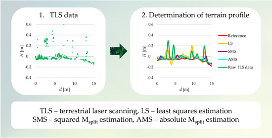
4.2. Real TLS Data
5. Discussion
6. Conclusions
Author Contributions
Funding
Institutional Review Board Statement
Informed Consent Statement
Data Availability Statement
Conflicts of Interest
References
- Błaszczak-Bąk, W.; Janowski, A.; Kamiński, W.; Rapiński, J. Application of the Msplit method for filtering airborne laser scanning data-sets to estimate digital terrain models. Int. J. Remote Sens. 2015, 36, 2421–2437. [Google Scholar] [CrossRef]
- Rodríguez-Gonzálvez, P.; Jiménez Fernández-Palacios, B.; Muñoz-Nieto, Á.L.; Arias-Sanchez, P.; Gonzalez-Aguilera, D. Mobile LiDAR System: New possibilities for the documentation and dissemination of large cultural heritage sites. Remote Sens. 2017, 9, 189. [Google Scholar] [CrossRef] [Green Version]
- Forlani, G.; Nardinocchi, C. Adaptive filtering of aerial laser scanning data. In Proceedings of the ISPRS Workshop on Laser Scanning 2007 and SilviLaser 2007, Espoo, Finland, 12–14 September 2007; pp. 130–135. [Google Scholar]
- Spaete, L.P.; Glenn, N.F.; Derryberry, D.R.; Sankey, T.T.; Mitchell, J.J.; Hardegree, S.P. Vegetation and slope effects on accuracy of a LiDAR-derived DEM in the sagebrush steppe. Remote Sens. Lett. 2011, 2, 317–326. [Google Scholar] [CrossRef]
- Zhao, X.; Guo, Q.; Su, Y.; Xue, B. Improved progressive TIN densification filtering algorithm for airborne LiDAR data in forested areas. ISPRS J. Photogramm. Remote Sens. 2016, 117, 79–91. [Google Scholar] [CrossRef] [Green Version]
- Crespo-Peremarch, P.; Tompalski, P.; Coops, N.C.; Ruiz, L.Á. Characterizing understory vegetation in Mediterranean forests using full-waveform airborne laser scanning data. Remote Sens. Environ. 2018, 217, 400–413. [Google Scholar] [CrossRef]
- Chen, C.; Li, Y. A fast global interpolation method for digital terrain model generation from large LiDAR-derived data. Remote Sens. 2019, 11, 1324. [Google Scholar] [CrossRef] [Green Version]
- Wang, C.; Hsu, P.-H. Building detection and structure line extraction from airborne LiDAR data. J. Photogramm. Remote Sens. 2007, 12, 365–379. [Google Scholar]
- He, M.; Zhu, Q.; Du, Z.; Hu, H.; Ding, Y.; Chen, M. A 3D shape descriptor based on contour clusters for damaged roof detection using airborne LiDAR point clouds. Remote Sens. 2016, 8, 189. [Google Scholar] [CrossRef] [Green Version]
- Zhang, Z.; Vosselman, G.; Gerke, M.; Persello, C.; Tuia, D.; Yang, M.Y. Detecting building changes between Airborne Laser Scanning and photogrammetric data. Remote Sens. 2019, 11, 2417. [Google Scholar] [CrossRef] [Green Version]
- Zhao, R.; Pang, M.; Liu, C.; Zhang, Y. Robust normal estimation for 3D LiDAR point clouds in urban environments. Sensors 2019, 19, 1248. [Google Scholar] [CrossRef] [Green Version]
- Błaszczak-Bąk, W.; Suchocki, C.; Janicka, J.; Dumalski, A.; Duchnowski, R.; Sobieraj-Żłobińska, A. Automatic threat detection for historic buildings in dark places based on the modified OptD method. ISPRS Int. J. Geo Inf. 2020, 9, 123. [Google Scholar] [CrossRef] [Green Version]
- Yang, H.; Omidalizarandi, M.; Xu, X.; Neumann, I. Terrestrial laser scanning technology for deformation monitoring and surface modeling of arch structures. Compos. Struct. 2017, 169, 173–179. [Google Scholar] [CrossRef] [Green Version]
- Zhao, X.; Kargoll, B.; Omidalizarandi, M.; Xu, X.; Alkhatib, H. Model selection for parametric surfaces approximating 3D point clouds for deformation analysis. Remote Sens. 2018, 10, 634. [Google Scholar] [CrossRef] [Green Version]
- Janicka, J.; Rapiński, J.; Błaszczak-Bąk, W.; Suchocki, C. Application of the Msplit estimation method in the detection and dimensioning of the displacement of adjacent planes. Remote Sens. 2020, 12, 3203. [Google Scholar] [CrossRef]
- Corso, J.; Roca, J.; Buill, F. Geometric analysis on stone façades with terrestrial laser scanner technology. Geosciences 2017, 7, 103. [Google Scholar] [CrossRef] [Green Version]
- Nurunnabi, A.; Belton, D.; West, G. Robust statistical approaches for local planar surface fitting in 3D laser scanning data. ISPRS J. Photogramm. Remote Sens. 2014, 96, 106–122. [Google Scholar] [CrossRef] [Green Version]
- Kwoczyńska, B.; Dobek, J. Elaboration of the 3D model and survey of the power lines using data from airborne laser scanning. J. Ecol. Eng. 2016, 17. [Google Scholar] [CrossRef]
- Suchocki, C. Conception of monitoring of cliff shores. Rep. Geod. 2011, 90, 461–467. [Google Scholar]
- Lian, X.; Hu, H. Terrestrial laser scanning monitoring and spatial analysis of ground disaster in Gaoyang coal mine in Shanxi, China: A technical note. Environ. Earth Sci. 2017, 76, 287. [Google Scholar] [CrossRef]
- Szwarkowski, D.; Moskal, M. Assessment of deformations in mining areas using the Riegl VZ-400 terrestrial laser scanner. E3S Web Conf. 2018, 36, 02009. [Google Scholar] [CrossRef]
- Janowski, A.; Rapiński, J. M-split estimation in laser scanning data modeling. J. Indian Soc. Remote Sens. 2013, 41, 15–19. [Google Scholar] [CrossRef]
- Carrilho, A.C.; Galo, M.; Santos, R.C. Statistical outlier detection method for airborne LiDAR data. In Proceedings of the ISPRS—International Archives of the Photogrammetry, Remote Sensing and Spatial Information Sciences, Karlsruhe, Germany, 10–12 October 2018; Copernicus GmbH: Göttingen, Germany, 2018; Volume XLII–1, pp. 87–92. [Google Scholar]
- Carrilho, A.C.; Galo, M. Automatic object extraction from high resolution aerial imagery with simple linear iterative clustering and convolutional neural networks. ISPRS—Int. Arch. Photogramm. Remote Sens. Spat. Inf. Sci. 2019, XLII-2/W16, 61–66. [Google Scholar] [CrossRef] [Green Version]
- Schnabel, R.; Wahl, R.; Klein, R. Efficient RANSAC for point-cloud shape detection. Comput. Graph. Forum 2007, 26, 214–226. [Google Scholar] [CrossRef]
- Nguyen, A.; Le, B. 3D point cloud segmentation: A survey. In Proceedings of the 2013 6th IEEE Conference on Robotics, Automation and Mechatronics (RAM), Manila, Phillippines, 12–15 November 2013; pp. 225–230. [Google Scholar]
- Li, L.; Yang, F.; Zhu, H.; Li, D.; Li, Y.; Tang, L. An improved RANSAC for 3D point cloud plane segmentation based on normal distribution transformation cells. Remote Sens. 2017, 9, 433. [Google Scholar] [CrossRef] [Green Version]
- Chen, Z.; Gao, B.; Devereux, B. State-of-the-art: DTM generation using airborne LIDAR data. Sensors 2017, 17, 150. [Google Scholar] [CrossRef] [PubMed] [Green Version]
- Wiśniewski, Z. Estimation of parameters in a split functional model of geodetic observations (Msplit estimation). J. Geod. 2009, 83, 105–120. [Google Scholar] [CrossRef]
- Wiśniewski, Z. Msplit(q) estimation: Estimation of parameters in a multi split functional model of geodetic observations. J. Geod. 2010, 84, 355–372. [Google Scholar] [CrossRef]
- Janowski, A. The circle object detection with the use of Msplit estimation. E3S Web Conf. 2018, 26, 00014. [Google Scholar] [CrossRef] [Green Version]
- Zienkiewicz, M.H.; Baryła, R. Determination of vertical indicators of ground deformation in the Old and Main City of Gdansk area by applying unconventional method of robust estimation. Acta Geodyn. Geomater. 2015, 12, 249–257. [Google Scholar] [CrossRef] [Green Version]
- Zienkiewicz, M.H.; Hejbudzka, K.; Dumalski, A. Multi split functional model of geodetic observations in deformation analyses of the Olsztyn castle. Acta Geodyn. Geomater. 2017, 14, 195–204. [Google Scholar] [CrossRef] [Green Version]
- Wyszkowska, P.; Duchnowski, R. Msplit estimation based on L1 norm condition. J. Surv. Eng. 2019, 145, 04019006. [Google Scholar] [CrossRef]
- Wyszkowska, P.; Duchnowski, R. Performance of Msplit estimates in the context of vertical displacement analysis. J. Appl. Geod. 2020, 14, 149–158. [Google Scholar] [CrossRef]
- Wyszkowska, P.; Duchnowski, R. Systematic bias of selected estimates applied in vertical displacement analysis. J. Geod. Sci. 2020, 10, 41–47. [Google Scholar] [CrossRef]
- Li, J.; Wang, A.; Xinyuan, W. Msplit estimate the relationship between LS and its application in gross error detection. Mine Surv. 2013, 2, 57–59. [Google Scholar] [CrossRef]
- Janicka, J.; Rapiński, J. Msplit transformation of coordinates. Surv. Rev. 2013, 45, 269–274. [Google Scholar] [CrossRef]
- Nowel, K. Squared Msplit(q) S-transformation of control network deformations. J. Geod. 2019, 93, 1025–1044. [Google Scholar] [CrossRef] [Green Version]
- Czaplewski, K.; Wąż, M.; Zienkiewicz, M.H. A novel approach of using selected unconventional geodesic methods of estimation on VTS areas. Mar. Geod. 2019, 42, 447–468. [Google Scholar] [CrossRef]
- Marshall, J.; Bethel, J. Basic concepts of L1 norm minimization for surveying applications. J. Surv. Eng. 1996, 122, 168–179. [Google Scholar] [CrossRef]
- Marshall, J. L1-norm pre-analysis measures for geodetic networks. J. Geod. 2002, 76, 334–344. [Google Scholar] [CrossRef]
- Wyszkowska, P.; Duchnowski, R. Iterative process of Msplit(q) estimation. J. Surv. Eng. 2020, 146, 06020002. [Google Scholar] [CrossRef]
- Duchnowski, R.; Wiśniewski, Z. Robustness of squared Msplit(q) estimation: Empirical analyses. Stud. Geophys. Geod. 2020, 64, 153–171. [Google Scholar] [CrossRef]
- Wiśniewski, Z.; Duchnowski, R.; Dumalski, A. Efficacy of Msplit estimation in displacement analysis. Sensors 2019, 19, 5047. [Google Scholar] [CrossRef] [PubMed] [Green Version]
- Zienkiewicz, M.H. Application of Msplit estimation to determine control points displacements in networks with unstable reference system. Surv. Rev. 2015, 47, 174–180. [Google Scholar] [CrossRef]


| Degree of Polynomial | Coefficients of Terms | ||||
|---|---|---|---|---|---|
| Two | - | - | 0.00300 | 0.04000 | 1.00000 |
| Three | - | 0.00050 | −0.00800 | −0.02000 | 1.00000 |
| Four | 0.00015 | −0.00594 | 0.07671 | −0.33062 | 0.50000 |
| Line | Variant | ||||||||||||
|---|---|---|---|---|---|---|---|---|---|---|---|---|---|
| LS | SMS | AMS | Raw TLS Data | LS | SMS | AMS | Raw TLS Data | LS | SMS | AMS | Raw TLS Data | ||
| I | A | 0.2634 | 0.1698 | 0.1875 | 0.3477 | 0.0609 | 0.0303 | 0.0251 | 0.0541 | 0.0367 | 0.0173 | 0.0157 | 0.0180 |
| B | 0.2548 | 0.1580 | 0.1569 | 0.0644 | 0.0301 | 0.0229 | 0.0417 | 0.0181 | 0.0172 | ||||
| C | 0.2083 | 0.3465 | 0.1620 | 0.0796 | 0.0795 | 0.0274 | 0.0707 | 0.0439 | 0.0224 | ||||
| D | 0.2293 | 0.4133 | 0.3592 | 0.0730 | 0.0558 | 0.0517 | 0.0551 | 0.0309 | 0.0244 | ||||
| II | A | 0.3124 | 0.5328 | 0.1580 | 0.2670 | 0.0459 | 0.0382 | 0.0218 | 0.0243 | 0.0184 | 0.0211 | 0.0089 | 0.0145 |
| B | 0.3161 | 0.1722 | 0.2088 | 0.0460 | 0.0254 | 0.0189 | 0.0180 | 0.0153 | 0.0089 | ||||
| C | 0.2625 | 0.0792 | 0.0411 | 0.0547 | 0.0270 | 0.0140 | 0.0164 | 0.0238 | 0.0124 | ||||
| D | 0.2378 | 0.1999 | 0.0346 | 0.0532 | 0.0400 | 0.0156 | 0.0174 | 0.0206 | 0.0159 | ||||
| Variant | ||||||||
|---|---|---|---|---|---|---|---|---|
| Line III | Line IV | |||||||
| LS | SMS | AMS | Raw TLS Data | LS | SMS | AMS | Raw TLS Data | |
| A | 0.0424 | 0.0374 | 0.0358 | 0.0409 | 0.0411 | 0.0375 | 0.0361 | 0.0403 |
| B | 0.0426 | 0.0376 | 0.0361 | 0.0412 | 0.0359 | 0.0354 | ||
| C | 0.0416 | 0.0389 | 0.0331 | 0.0407 | 0.0387 | 0.0336 | ||
| D | 0.0427 | 0.0431 | 0.0385 | 0.0419 | 0.0354 | 0.0363 | ||
| Variant | ||||||||||||
|---|---|---|---|---|---|---|---|---|---|---|---|---|
| LS | SMS | AMS | Raw TLS Data | LS | SMS | AMS | Raw TLS Data | LS | SMS | AMS | Raw TLS Data | |
| A | 0.0523 | 0.0483 | 0.0361 | 0.0595 | 0.0159 | 0.0157 | 0.0127 | 0.0174 | 0.0115 | 0.0119 | 0.0087 | 0.0138 |
| B | 0.0460 | 0.0438 | 0.0520 | 0.0171 | 0.0155 | 0.0154 | 0.0125 | 0.0137 | 0.0118 | |||
| C | 0.0620 | 0.0900 | 0.0468 | 0.0171 | 0.0211 | 0.0131 | 0.0144 | 0.0175 | 0.0111 | |||
| D | 0.0396 | 0.0803 | 0.0695 | 0.0136 | 0.0217 | 0.0143 | 0.0113 | 0.0148 | 0.0122 | |||
Publisher’s Note: MDPI stays neutral with regard to jurisdictional claims in published maps and institutional affiliations. |
© 2020 by the authors. Licensee MDPI, Basel, Switzerland. This article is an open access article distributed under the terms and conditions of the Creative Commons Attribution (CC BY) license (http://creativecommons.org/licenses/by/4.0/).
Share and Cite
Wyszkowska, P.; Duchnowski, R.; Dumalski, A. Determination of Terrain Profile from TLS Data by Applying Msplit Estimation. Remote Sens. 2021, 13, 31. https://doi.org/10.3390/rs13010031
Wyszkowska P, Duchnowski R, Dumalski A. Determination of Terrain Profile from TLS Data by Applying Msplit Estimation. Remote Sensing. 2021; 13(1):31. https://doi.org/10.3390/rs13010031
Chicago/Turabian StyleWyszkowska, Patrycja, Robert Duchnowski, and Andrzej Dumalski. 2021. "Determination of Terrain Profile from TLS Data by Applying Msplit Estimation" Remote Sensing 13, no. 1: 31. https://doi.org/10.3390/rs13010031