Hyperspectral Estimation of Soil Organic Matter Content using Different Spectral Preprocessing Techniques and PLSR Method

 ,
, 
Abstract
:
1. Introduction
2. Materials and Methods
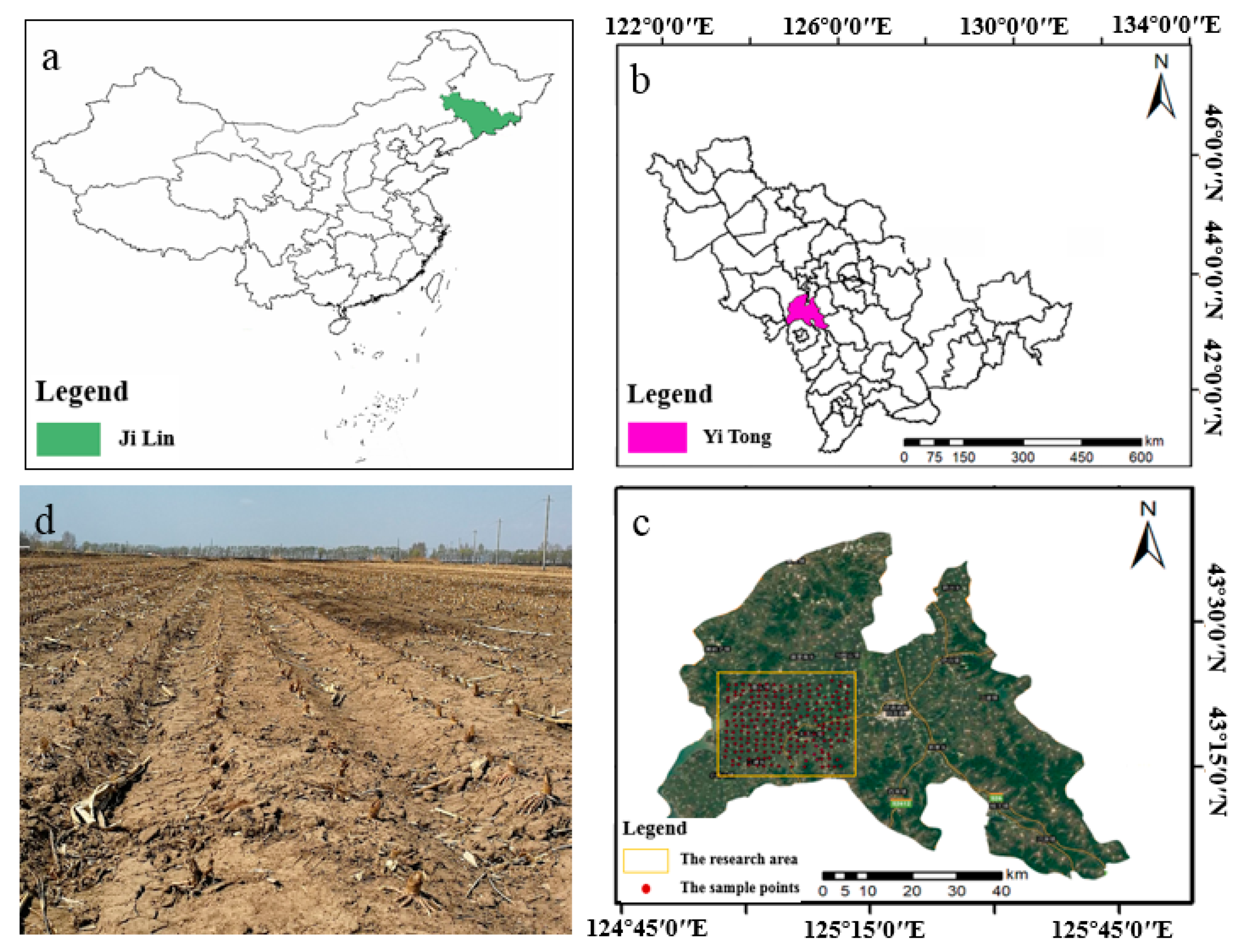
2.1. Study Area and Soil Sample Collection
2.2. Spectral Measurements
2.3. Description of Sample Set
2.4. Preprocessing Methods
2.4.1. Savitzky–Golay Denoising
2.4.2. Wavelet Packet Denoising
2.4.3. Mathematical Transformations of Spectral Reflectance Data
2.4.4. PCA Dimensionality Reduction
2.4.5. Sensitive Band Dimensionality Reduction
2.5. Partial Least Squares Regression Method
2.6. Metrics for Evaluating Model Performance
3. Results and Discussion
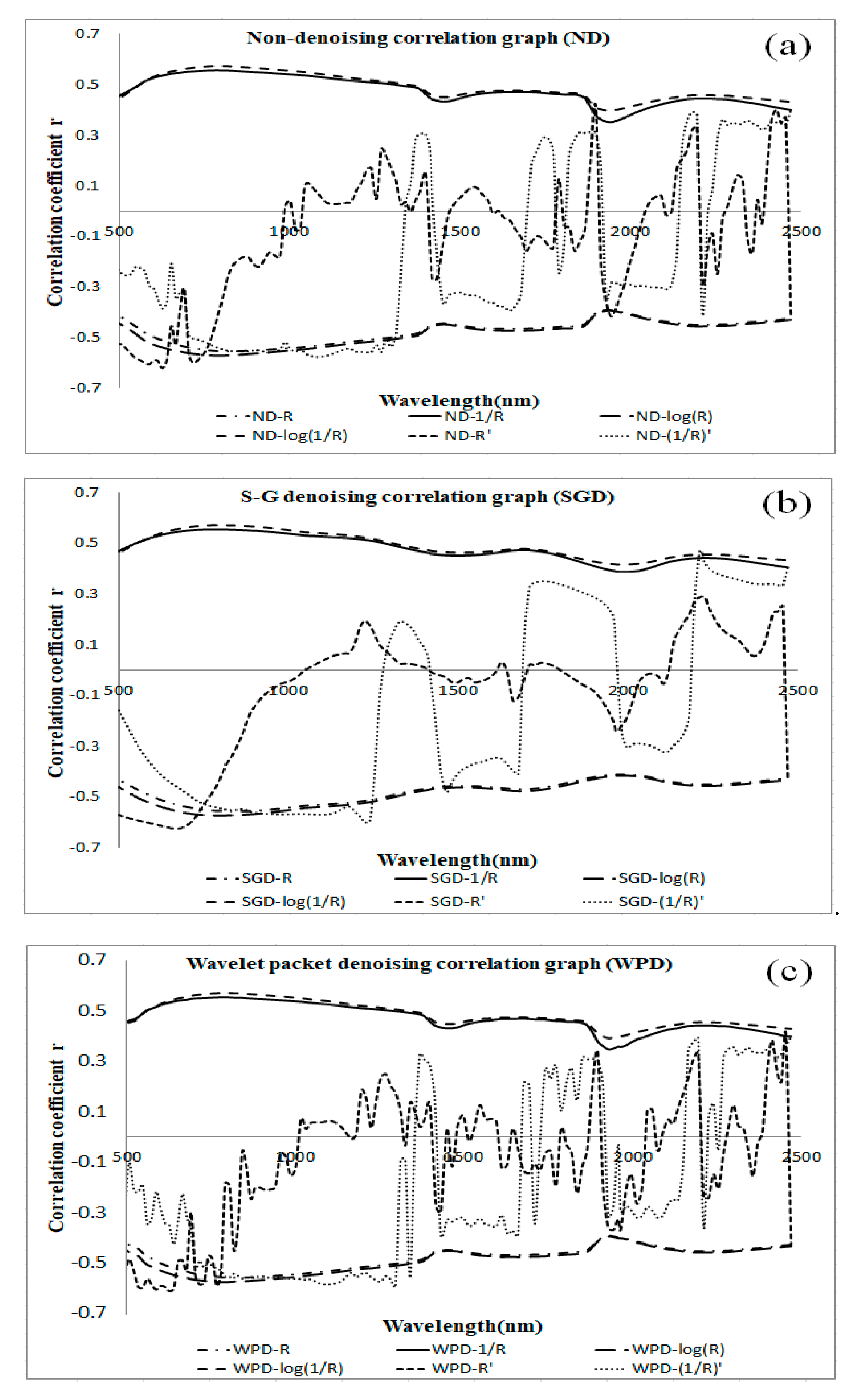
3.1. Correlation between SOM Content and Reflectance Data Subjected to Different Pretreatments
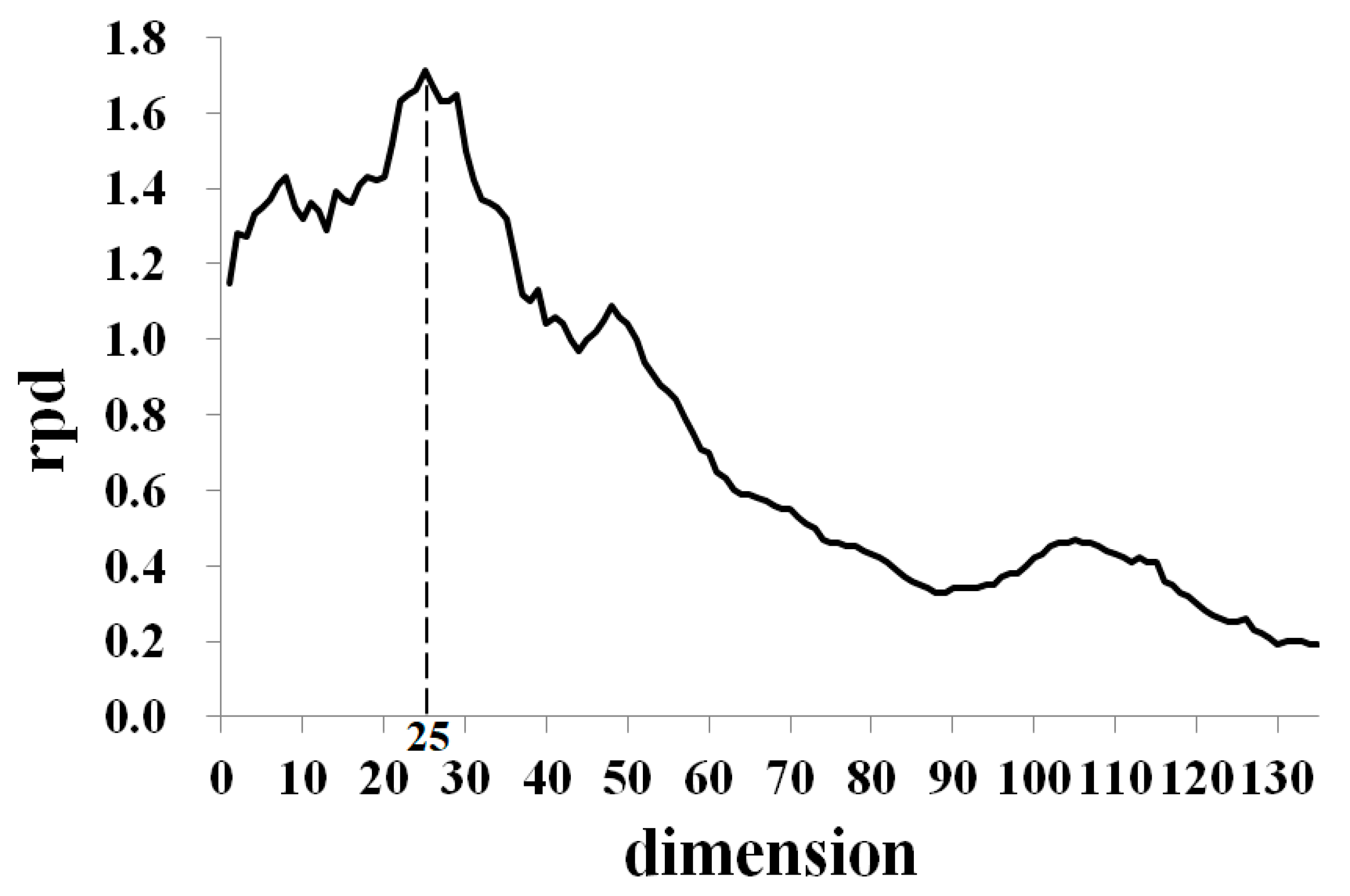
3.2. Determination of Optimal Parameter Value for PCA
3.3. Accuracy Analysis of the Hyperspectral Estimation Model of theSOM Content based on PLSR
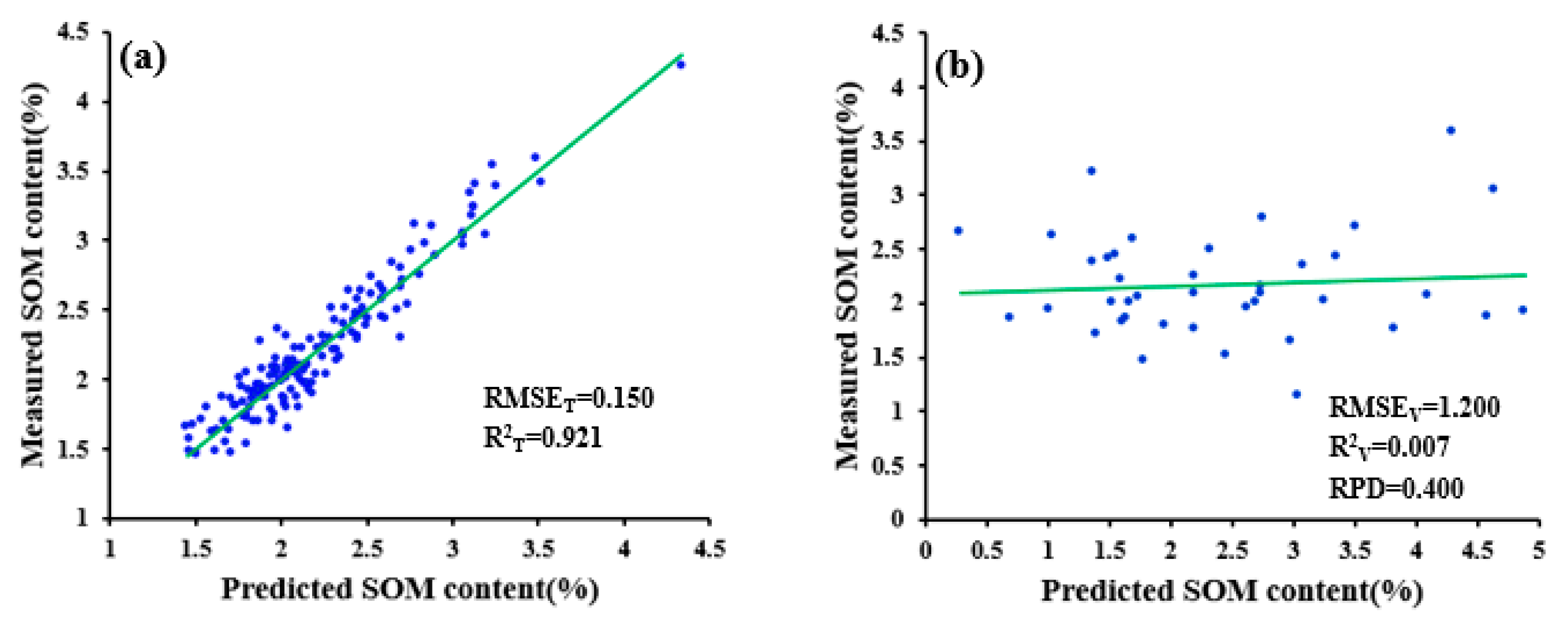
3.3.1. Comparison of the Modeling Results based on Original Data and Data Obtained after Effective Pretreatment
3.3.2. Comparison of Modeling Results for Different Dimensionality Reduction Methods
3.3.3. Comparison of Modeling Results for Different Denoising Methods
3.3.4. Discussion of Different Preprocessing Techniques for Soil Hyperspectral Data
4. Conclusions
Author Contributions
Funding
Acknowledgments
Conflicts of Interest
References
- Munson, S.A.; Carey, A.E. Organic matter sources and transport in an agricultural dominated temperate watershed. Appl. Geochem. 2004, 19, 1111–1121. [Google Scholar] [CrossRef]
- Dou, S. Soil Organic Matter; Science Press: Beijing, China, 2010. [Google Scholar]
- Alexakis, D.; Tapoglou, E.; Vozinaki, A.E.; Tsanis, I.K. Integrated Use of Satellite Remote Sensing, Artificial Neural Networks, Field Spectroscopy, and GIS in Estimating Crucial Soil Parameters in Terms of Soil Erosion. Remote Sens. 2019, 11, 1106. [Google Scholar] [CrossRef] [Green Version]
- Kawamura, K.; Tsujimoto, Y.; Nishigaki, T.; Andriamananjara, A.; Rabenarivo, M.; Asai, H.; Razafimbelo, T. Laboratory Visible and Near-Infrared Spectroscopy with Genetic Algorithm-Based Partial Least Squares Regression for Assessing the Soil Phosphorus Content of Upland and Lowland Rice Fields in Madagascar. Remote Sens. 2019, 11, 506. [Google Scholar] [CrossRef] [Green Version]
- Gholizadeh, A.; Saberioon, M.; Carmon, N.; Boruvka, L.; Ben-Dor, E. Examining the Performance of PARACUDA-II Data-Mining Engine versus Selected Techniques to Model Soil Carbon from Reflectance Spectra. Remote Sens. 2018, 10, 1172. [Google Scholar] [CrossRef] [Green Version]
- Kopacková, V.; Eyal, B.D.; Nimrod, C.; Notesco, G. Modelling Diverse Soil Attributes with Visible to Longwave Infrared Spectroscopy Using PLSR Employed by an Automatic Modelling Engine. Remote Sens. 2017, 9, 134. [Google Scholar] [CrossRef] [Green Version]
- Rossel, R.A.V.; Walvoort, D.J.J.; Mcbratney, A.B.; Janik, L.J.; Skjemstad, J.O. Visible, near infrared, mid infrared or combined diffuse reflectance spectroscopy for simultaneous assessment of various soil properties. Geoderma 2006, 131, 59–75. [Google Scholar] [CrossRef]
- Peón, J.; Carmen, R.; Fernández, S.; Calleja, J.F.; De Miguel, E.; Carretero, L. Prediction of Topsoil Organic Carbon Using Airborne and Satellite Hyperspectral Imagery. Remote Sens. 2017, 9, 1211. [Google Scholar] [CrossRef] [Green Version]
- Liu, X.M. Near infrared diffuse reflectance spectra detection of soil organic matter and available N. J. Chin. Agric. Mech. 2013, 34, 202–206. [Google Scholar]
- Liu, Y.; Liu, Y.L.; Chen, Y.Y.; Zhang, Y.; Shi, T.; Wang, J.; Fei, T. The Influence of Spectral Pretreatment on the Selection of Representative Calibration Samples for Soil Organic Matter Estimation Using Vis-NIR Reflectance Spectroscopy. Remote Sens. 2019, 11, 450. [Google Scholar] [CrossRef] [Green Version]
- Zhang, S.; Shen, Q.; Nie, C.; Huang, Y.; Wang, J.; Hu, Q.; Chen, Y. Hyperspectral inversion of heavy metal content in reclaimed soil from a mining wasteland based on different spectral transformation and modeling methods. Spectrochim. Acta Part A Mol. Biomol. Spectrosc. 2018, 211, 393–400. [Google Scholar] [CrossRef]
- Vohland, M.; Ludwig, M.; Thiele-Bruhn, S.; Ludwig, B. Quantification of Soil Properties with Hyperspectral Data: Selecting Spectral Variables with Different Methods to Improve Accuracies and Analyze Prediction Mechanisms. Remote Sens. 2017, 9, 1103. [Google Scholar] [CrossRef] [Green Version]
- Dong, C.W. Face Recognition Based on PCA and SVM Algorithm. Radio Telev. Inf. 2018, 10, 107–110. [Google Scholar]
- Sahrawat, K.L. Simple modification of the Walkley-Black method for simultaneous determination of organic carbon and potentially mineralizable nitrogen in tropical rice soils. Plant Soil. 1982, 69, 73–77. [Google Scholar] [CrossRef]
- Feng, Y.S.; Wu, P.X.; Liu, Y.J.; Zhou, B.J.; Ma, J. The Study of The Soil Spectral Characteristics. J. Jilin Agric. Univ. 1989, 11, 72–76. [Google Scholar]
- Peng, J.; Zhang, Y.Z.; Zhou, Q. Spectral Characteristics of Soils in Hunan Province as Affected by Removal of Soil Organic Matter. Soils 2006, 38, 453–458. [Google Scholar]
- Steinier, J.; Termonia, Y.; Deltour, J. Smoothing and differentiation of data by simplified least square procedure. Anal. Chem. 1972, 44, 1906–1909. [Google Scholar] [CrossRef]
- Askari, M.S.; Cui, J.F.; O’Rourke, S.M.; Holden, N.M. Evaluation of soil structural quality using VIS–NIR spectra. Soil Tillage Res. 2015, 146, 108–117. [Google Scholar] [CrossRef]
- Hook, J. Smoothing non-smooth systems with low-pass filters. Phys. D Nonlinear Phenom. 2014, 269, 76–85. [Google Scholar] [CrossRef]
- Huang, Y.H.; Wang, J.H.; Jiang, D.; Zhou, Q. Reconstruction of MODIS-EVI Time-Series Data with S-G Filter. Geomat. Inf. Sci. Wuhan Univ. 2009, 34, 1440–1443. [Google Scholar]
- Savitzky, A.; Golay, M.J.E. Smoothing and differentiation of data by simplified least squares procedures. Anal. Chem. 1964, 36, 1627–1639. [Google Scholar] [CrossRef]
- Yang, H.; Shen, R.P.; Wu, L.Y.; Li, M. Temporal and Spatial Analysis of Remotely Sensed Vegetation Coverage Changes in Jiangxi Province Based on S-G Filter. Sci. Technol. Eng. 2014, 14, 101–106. [Google Scholar]
- Kong, L.J. Matlab Wavelet Analysis Super Learning Manual; The People’s Posts and Telecommunications Press: Beijing, China, 2014. [Google Scholar]
- Virmani, J.; Kumar, V.; Kalar, N.; Khandelwal, N. SVM-Based Characterization of Liver Ultrasound Images Using Wavele Packet Texture Descriptors. J. Digit. Imaging 2012, 26, 530–543. [Google Scholar] [CrossRef] [PubMed] [Green Version]
- Rivera-Caicedo, J.P.; Jochem, V.; Jordi, M.; Camps-Valls, G.; Moreno, J. Hyperspectral dimensionality reduction for biophysical variable statistical retrieval. ISPRS J. Photogramm. Remote Sens. 2017, 132, 88–101. [Google Scholar] [CrossRef]
- Pearson, K. On lines and planes of closest fit to systems of points in space. Phil. Mag. 1901, 2, 559–572. [Google Scholar] [CrossRef] [Green Version]
- Goodarzi, M.; Sharma, S.; Ramon, H.; Saeys, W. Multivariate calibration of NIR spectroscopic sensors for continuous glucose monitoring. TrAC Trends Anal. Chem. 2015, 67, 147–158. [Google Scholar] [CrossRef] [Green Version]
- Giacomo, D.R.; Stefania, D.Z. A multivariate regression model for detection of fumonisins content in maize from near infrared spectra. Food Chem. 2013, 141, 4289–4294. [Google Scholar] [CrossRef]
- Wang, F.H.; Gao, J.; Zha, Y. Hyperspectral sensing of heavy metals in soil and vegetation: Feasibility and challenges. ISPRS J. Photogramm. Remote Sens. 2018, 136, 73–84. [Google Scholar] [CrossRef]
- Chang, C.W.; Laird, A.D.; Mausbach, M.J.; Hurburgh, C.R. Near infrared reflectance spectroscopy: Principal components regression analysis of soil properties. Soil Sci. Soc. Am. J. 2001, 65, 480–490. [Google Scholar] [CrossRef] [Green Version]
- Qiao, X.X.; Wang, C.; Feng, M.C.; Yang, W.D.; Ding, G.W.; Sun, H.; Shi, C.C. Hyperspectral estimation of soil organic matter based on different spectral preprocessing techniques. Spectrosc. Lett. 2017, 50, 156–163. [Google Scholar] [CrossRef]
- Wang, X.; Zhang, F.; Kung, H.T.; Johnson, V.C. New methods for improving the remote sensing estimation of soil organic matter content (SOMC) in the Ebinur Lake Wetland National Nature Reserve (ELWNNR) in northwest China. Remote Sens. Environ. 2018, 218, 104–118. [Google Scholar] [CrossRef]
- Pineiro, G.; Perelman, S.; Guerschman, J.P.; Paruelo, J.M. How to evaluate models: Observed vs. predicted or predicted vs. observed? Ecol. Model. 2008, 216, 316–322. [Google Scholar] [CrossRef]
- Baumgardner, M.F. Reflectance properties of soils. Adv. Agron. 1985, 38, 1–44. [Google Scholar]
- Zheng, G.H.; Ryu, D.; Jiao, C.Q. Estimation of Organic Matter Content in Coastal Soil Using Reflectance Spectroscopy. Pedosphere 2016, 26, 130–136. [Google Scholar] [CrossRef]
- Wang, J.; He, T.; Lv, C.Y.; Chen, Y.; Jian, W. Mapping soil organic matter based on land degradation spectral response units using Hyperion images. Int. J. Appl. Earth Obs. Geoinf. 2010, 12 (Suppl. 2), S171–S180. [Google Scholar] [CrossRef]
- Nocita, M.; Stevens, A.; Toth, G.; Panagos, P.; van Wesemael, B.; Montanarella, L. Prediction of soil organic carbon content by diffuse reflectance spectroscopy using a local partial least square regression approach. Soil Biol. Biochem. 2014, 68, 337–347. [Google Scholar] [CrossRef]
- Mouazen, A.M.; Maleki, M.R.; Baerdemaeker, J.D.; Ramon, H. On-line measurement of some selected soil properties using a VIS–NIR sensor. Soil Tillage Res. 2007, 93, 13–27. [Google Scholar] [CrossRef]
- Luce, M.S.; Ziadi, N.; Zebarth, B.J.; Grant, C.A.; Tremblay, G.F.; Gregorich, E.G. Rapid determination of soil organic matter quality indicators using visible near infrared reflectance spectroscopy. Geoderma 2014, 232–234, 449–458. [Google Scholar]
- Ben-Dor, E.; Banin, A. Near-infrared analysis as a rapid method to simultaneously evaluate several soil properties. Soil Sci. Soc. Am. J. 1995, 159, 259–270. [Google Scholar] [CrossRef]
- Chabrillat, S.; Goetz, A.F.H.; Krosley, L.; Olsen, H.W. Use of hyperspectral images in the identification and mapping of expansive clay soils and the role of spatial resolution. Remote Sens. Environ. 2002, 82, 431–445. [Google Scholar] [CrossRef]
- Barnes, R.J.; Dhanoa, M.S.; Lister, S.J. Standard Normal Variate Transformation and De-Trending of Near-Infrared Diffuse Reflectance Spectra. Appl. Spectrosc. 1989, 43, 772–777. [Google Scholar] [CrossRef]
- Chen, H.Z.; Song, Q.Q.; Tang, G.Q.; Feng, Q.X.; Lin, L. The Combined Optimization of Savitzky-Golay Smoothing and Multiplicative Scatter Correction for FT-NIR PLS Models. ISRN Spectrosc. 2013, 1–9. [Google Scholar] [CrossRef] [Green Version]
- Oldham, K.B.; Spanier, J. The fractional calculus. Math. Gazette. 1974, 56, 396–400. [Google Scholar]
- Li, B.; Xie, W. Adaptive fractional differential approach and its application to medical image enhancement. Comput. Electr. Eng. 2015, 45, 324–335. [Google Scholar] [CrossRef]


| Sample Set | No. of Samples | SOM (%) | |||
|---|---|---|---|---|---|
| Max | Min | Ave | Std | ||
| Total samples Training dataset Validation dataset | 198 158 40 | 4.254 4.254 3.589 | 1.150 1.458 1.150 | 2.203 2.212 2.170 | 0.495 0.499 0.486 |
| Denoising methods | ND, SGD, WPD |
| Data transformations | R, 1/R, log(R), log(1/R), R’, (1/R)’ |
| Dimensionality reduction methods | NDR, SWDR, PCADR |
| Pretreatment Methods Used | Denoising Methods | |||
|---|---|---|---|---|
| ND | SGD | WPD | ||
| Data transformations performed on spectral data | R | ND-R | SGD-R | WPD-R |
| 1/R | ND-1/R | SGD-1/R | WPD-1/R | |
| log(R) | ND-log(R) | SGD-log(R) | WPD-log(R) | |
| log(1/R) | ND-log(1/R) | SGD-log(1/R) | WPD-log(1/R) | |
| R’ | ND-R’ | SGD-R’ | WPD-R’ | |
| (1/R)’ | ND-(1/R)’ | SGD-(1/R)’ | WPD-(1/R)’ | |
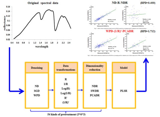
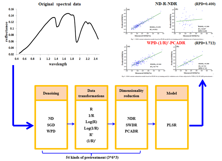
| Pretreatment Method | RMSET (%) | RMSEV (%) | R2T | R2V | RPD | ||
|---|---|---|---|---|---|---|---|
| ND | R | NDR | 0.150 | 1.200 | 0.921 | 0.007 | 0.400 |
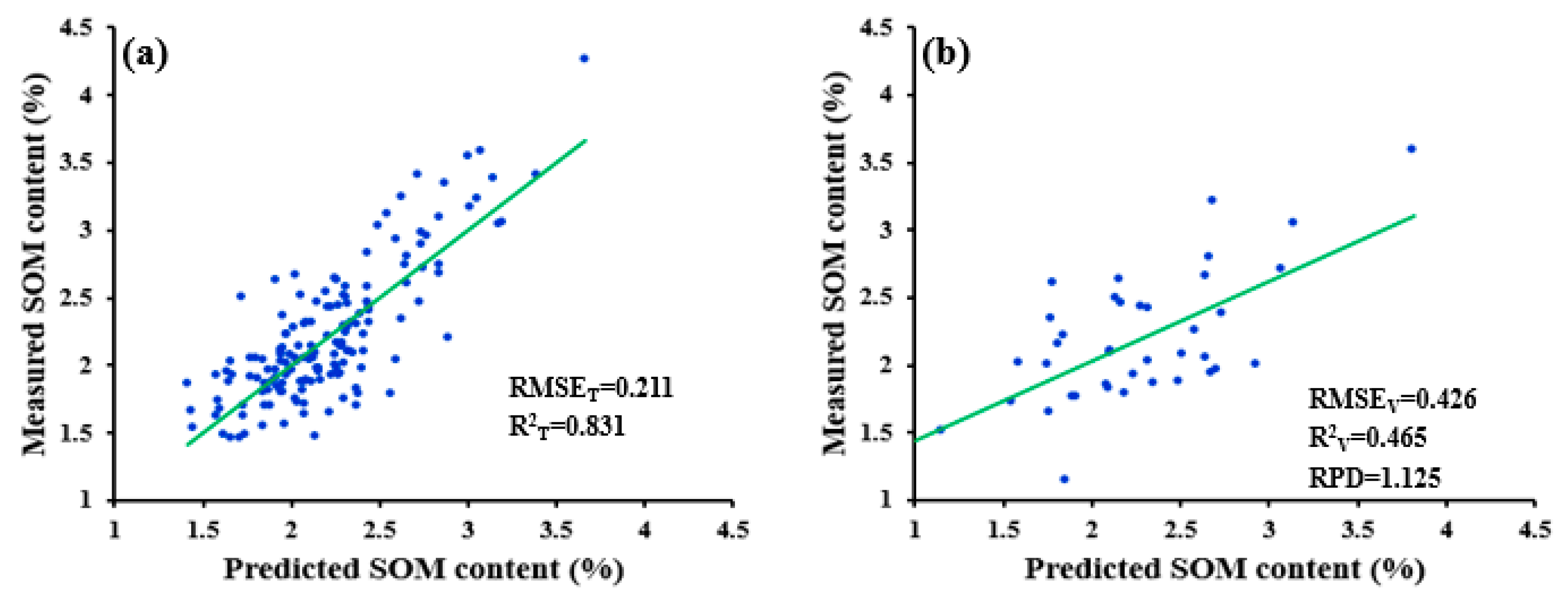
| SWDR | 0.211 | 0.426 | 0.831 | 0.465 | 1.125 | ||
| PCADR | 0.320 | 0.350 | 0.595 | 0.512 | 1.370 | ||
| 1/R | NDR | 0.113 | 0.934 | 0.950 | 0.229 | 0.660 | |
| SWDR | 0.269 | 0.605 | 0.718 | 0.508 | 0.793 | ||
| PCADR | 0.338 | 0.326 | 0.544 | 0.589 | 1.472 | ||
| log(R) | NDR | 0.128 | 0.903 | 0.946 | 0.054 | 0.531 | |
| SWDR | 0.266 | 0.420 | 0.723 | 0.556 | 1.141 | ||
| PCADR | 0.325 | 0.301 | 0.582 | 0.640 | 1.591 | ||
| log(1/R) | NDR | 0.128 | 0.903 | 0.946 | 0.054 | 0.531 | |
| SWDR | 0.266 | 0.420 | 0.723 | 0.556 | 1.141 | ||
| PCADR | 0.325 | 0.301 | 0.582 | 0.640 | 1.591 | ||
| R’ | NDR | 0.150 | 0.200 | 0.921 | 0.007 | 0.400 | |
| SWDR | 0.335 | 0.417 | 0.553 | 0.323 | 1.150 | ||
| PCADR | 0.317 | 0.338 | 0.602 | 0.533 | 1.419 | ||
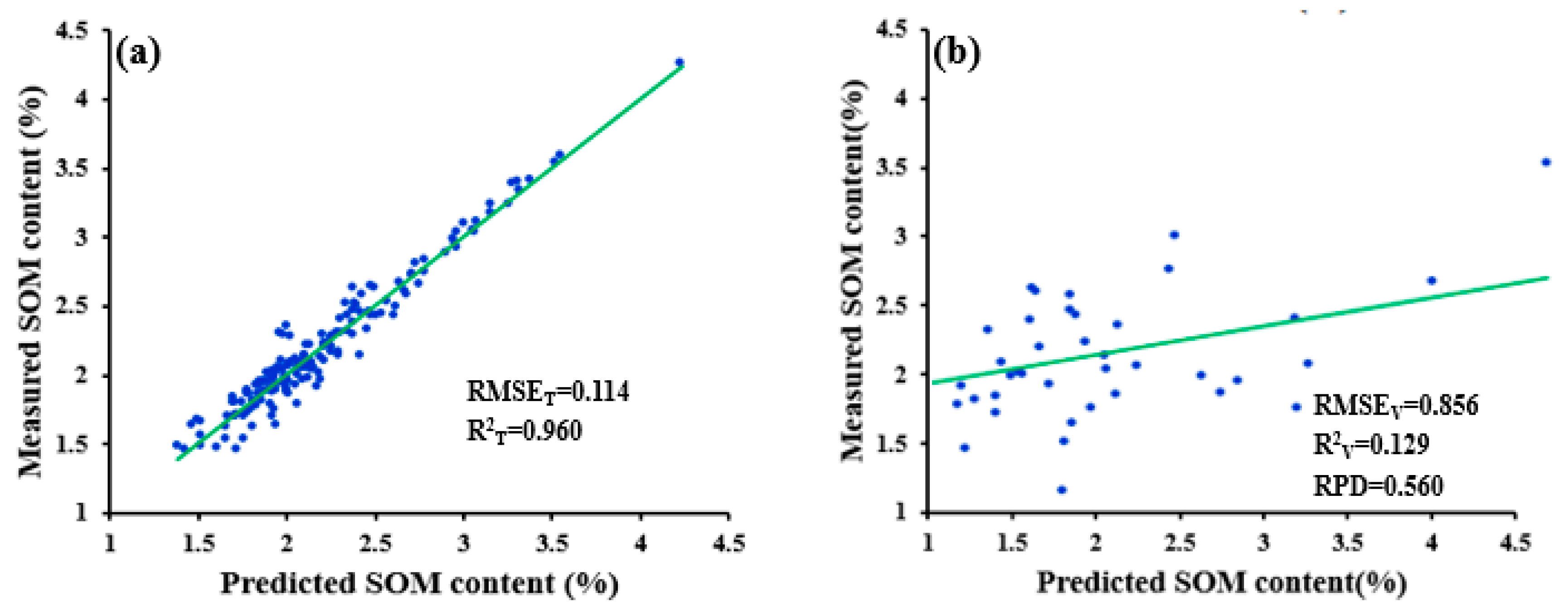
| (1/R)’ | NDR | 0.114 | 0.856 | 0.960 | 0.129 | 0.560 | |
| SWDR | 0.293 | 0.568 | 0.660 | 0.400 | 0.844 | ||
| PCADR | 0.330 | 0.331 | 0.568 | 0.555 | 1.449 | ||
| SGD | R | NDR | 0.208 | 0.817 | 0.836 | 0.110 | 0.586 |
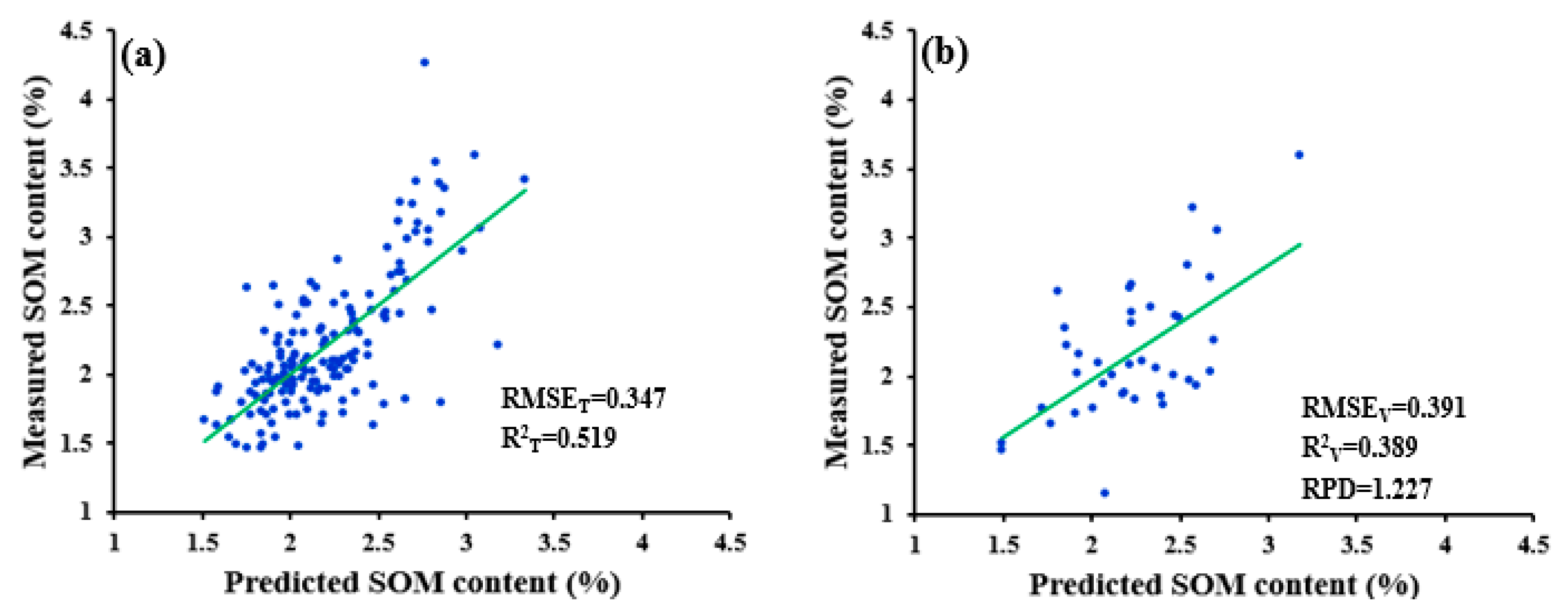
| SWDR | 0.347 | 0.391 | 0.519 | 0.389 | 1.227 | ||
| PCADR | 0.285 | 0.348 | 0.680 | 0.538 | 1.377 | ||
| 1/R | NDR | 0.141 | 1.031 | 0.932 | 0.147 | 0.465 | |
| SWDR | 0.386 | 0.424 | 0.402 | 0.289 | 1.130 | ||
| PCADR | 0.341 | 0.311 | 0.537 | 0.627 | 1.542 | ||
| log(R) | NDR | 0.148 | 1.014 | 0.923 | 0.127 | 0.473 | |
| SWDR | 0.304 | 0.354 | 0.633 | 0.526 | 1.352 | ||
| PCADR | 0.344 | 0.321 | 0.528 | 0.585 | 1.494 | ||
| log(1/R) | NDR | 0.148 | 1.014 | 0.923 | 0.127 | 0.473 | |
| SWDR | 0.304 | 0.354 | 0.633 | 0.526 | 1.352 | ||
| PCADR | 0.344 | 0.321 | 0.528 | 0.585 | 1.494 | ||
| R’ | NDR | 0.204 | 0.710 | 0.842 | 0.176 | 0.675 | |
| SWDR | 0.351 | 0.343 | 0.507 | 0.532 | 1.398 | ||
| PCADR | 0.337 | 0.344 | 0.548 | 0.516 | 1.392 | ||
| (1/R)’ | NDR | 0.141 | 1.032 | 0.932 | 0.147 | 0.465 | |
| SWDR | 0.336 | 0.436 | 0.551 | 0.396 | 1.101 | ||
| PCADR | 0.309 | 0.334 | 0.623 | 0.593 | 1.434 | ||
| WPD | R | NDR | 0.211 | 0.834 | 0.831 | 0.111 | 0.575 |
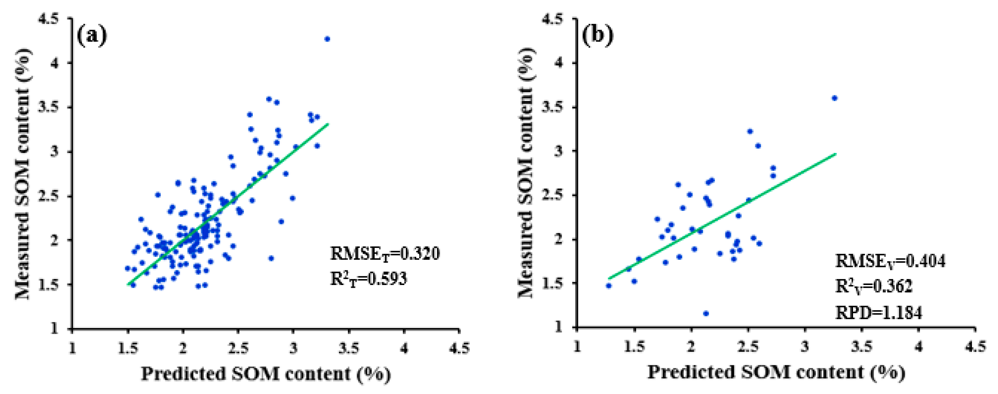
| SWDR | 0.320 | 0.404 | 0.593 | 0.362 | 1.184 | ||
| PCADR | 0.271 | 0.346 | 0.713 | 0.563 | 1.386 | ||
| 1/R | NDR | 0.114 | 0.856 | 0.960 | 0.129 | 0.560 | |
| SWDR | 0.243 | 0.614 | 0.770 | 0.371 | 0.781 | ||
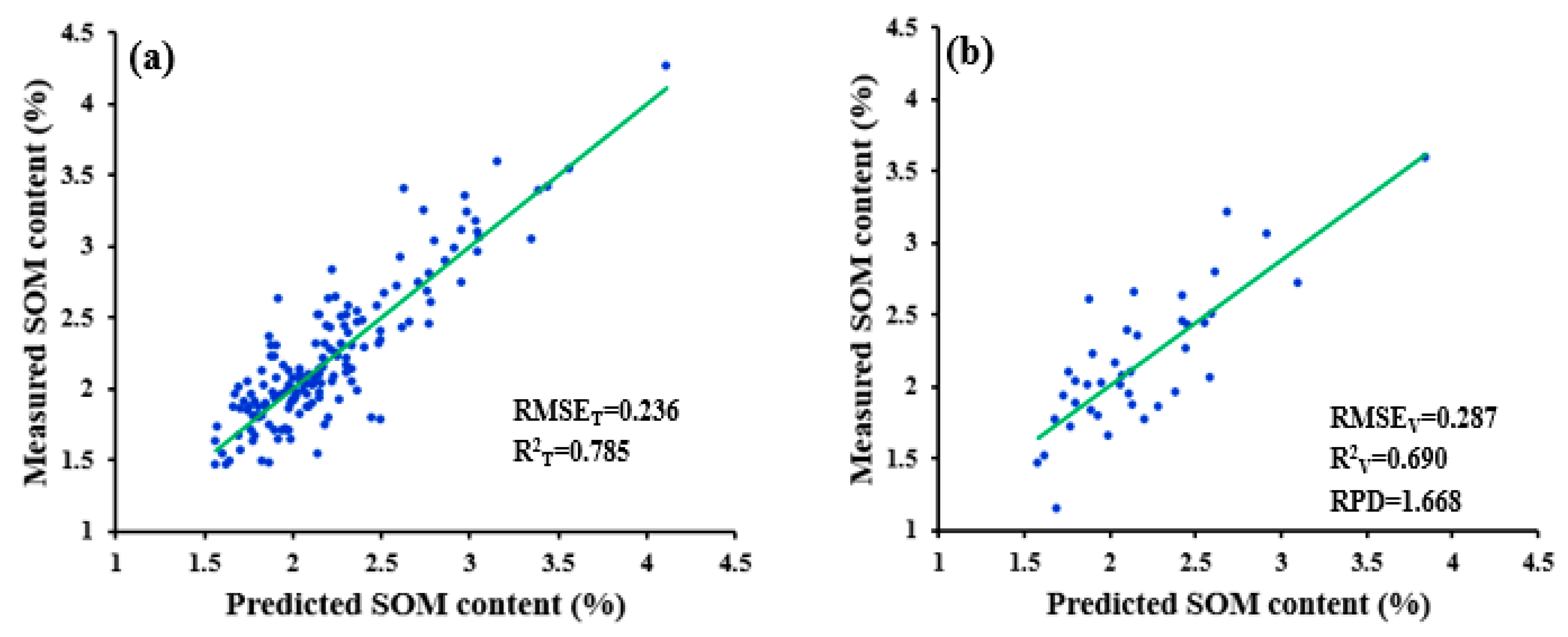
| PCADR | 0.236 | 0.287 | 0.785 | 0.690 | 1.668 | ||
| log(R) | NDR | 0.121 | 1.384 | 0.953 | 0.038 | 0.346 | |
| SWDR | 0.249 | 0.581 | 0.759 | 0.0.279 | 0.825 | ||
| PCADR | 0.239 | 0.306 | 0.780 | 0.642 | 1.569 | ||
| log(1/R) | NDR | 0.121 | 1.384 | 0.953 | 0.038 | 0.346 | |
| SWDR | 0.249 | 0.581 | 0.759 | 0.0.279 | 0.825 | ||
| PCADR | 0.239 | 0.306 | 0.780 | 0.642 | 1.569 | ||
| R’ | NDR | 0.211 | 2.885 | 0.831 | 0.0001 | 0.166 | |
| SWDR | 0.299 | 0.343 | 0.646 | 0.530 | 1.399 | ||
| PCADR | 0.299 | 0.343 | 0.646 | 0.530 | 1.399 | ||
| (1/R)’ | NDR | 0.108 | 2.421 | 0.965 | 0.0004 | 0.198 | |
| SWDR | 0.295 | 0.451 | 0.657 | 0.303 | 1.064 | ||
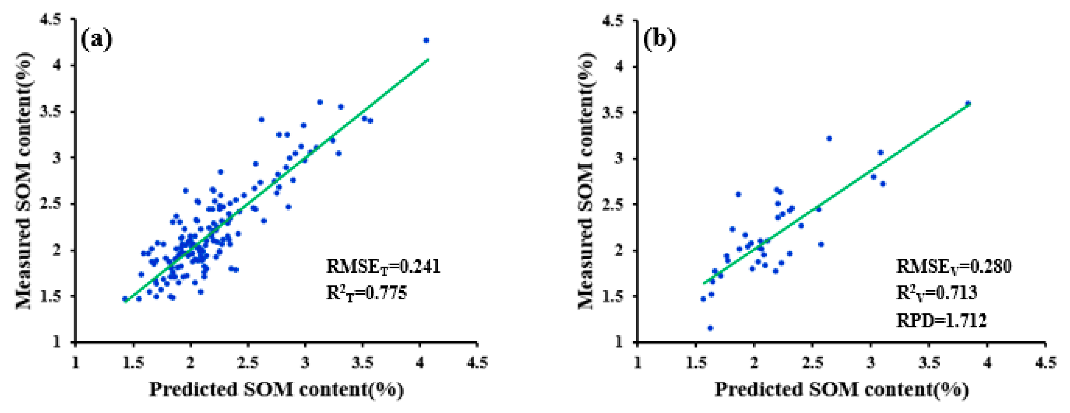
| PCADR | 0.241 | 0.280 | 0.775 | 0.713 | 1.712 | ||
| Pretreatment Method | RMSET (%) | RMSEV (%) | R2T | R2V | RPD |
|---|---|---|---|---|---|
| No pretreatment | 0.150 | 1.200 | 0.921 | 0.007 | 0.400 |
| WPD-(1/R)’-PCADR | 0.241 | 0.280 | 0.775 | 0.713 | 1.712 |
| Pretreatment Method | RMSET (%) | RMSEV (%) | R2T | R2V | RPD |
|---|---|---|---|---|---|
| WPD-1/R-NDR | 0.114 | 0.856 | 0.960 | 0.129 | 0.560 |
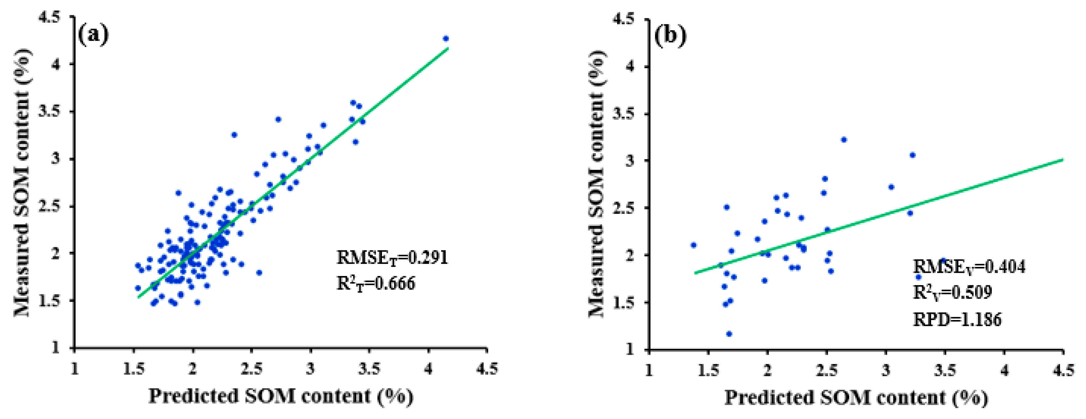
| WPD-1/R-SWDR | 0.291 | 0.404 | 0.666 | 0.509 | 1.186 |
| WPD-1/R-PCADR | 0.236 | 0.287 | 0.785 | 0.690 | 1.668 |
| Pretreatment Method | RMSET (%) | RMSEV (%) | R2T | R2V | RPD |
|---|---|---|---|---|---|
| ND-R-SWDR | 0.211 | 0.426 | 0.831 | 0.465 | 1.125 |
| SGD-R-SWDR | 0.347 | 0.391 | 0.519 | 0.389 | 1.227 |
| WPD-R-SWDR | 0.320 | 0.404 | 0.593 | 0.362 | 1.184 |
© 2020 by the authors. Licensee MDPI, Basel, Switzerland. This article is an open access article distributed under the terms and conditions of the Creative Commons Attribution (CC BY) license (http://creativecommons.org/licenses/by/4.0/).
Share and Cite
Shen, L.; Gao, M.; Yan, J.; Li, Z.-L.; Leng, P.; Yang, Q.; Duan, S.-B. Hyperspectral Estimation of Soil Organic Matter Content using Different Spectral Preprocessing Techniques and PLSR Method. Remote Sens. 2020, 12, 1206. https://doi.org/10.3390/rs12071206
Shen L, Gao M, Yan J, Li Z-L, Leng P, Yang Q, Duan S-B. Hyperspectral Estimation of Soil Organic Matter Content using Different Spectral Preprocessing Techniques and PLSR Method. Remote Sensing. 2020; 12(7):1206. https://doi.org/10.3390/rs12071206
Chicago/Turabian StyleShen, Lanzhi, Maofang Gao, Jingwen Yan, Zhao-Liang Li, Pei Leng, Qiang Yang, and Si-Bo Duan. 2020. "Hyperspectral Estimation of Soil Organic Matter Content using Different Spectral Preprocessing Techniques and PLSR Method" Remote Sensing 12, no. 7: 1206. https://doi.org/10.3390/rs12071206