Article

Use of Uncertainty Inflation in OSTIA to Account for Correlated Errors in Satellite-Retrieved Sea Surface Temperature Data

Met Office, FitzRoy Road, Exeter, Devon EX1 3PB, UK
*
Author to whom correspondence should be addressed.
Remote Sens. 2020, 12(7), 1083; https://doi.org/10.3390/rs12071083
Submission received: 26 February 2020 / Accepted: 21 March 2020 / Published: 27 March 2020

Abstract

:
Sea surface temperature (SST) analysis systems such as the Operational Sea Surface Temperature and Ice Analysis (OSTIA) use statistical methods to combine observations together with a first guess field to create spatially complete maps of SST. These commonly assume that observation errors are uncorrelated, yet some errors (such as due to retrieval issues) can be correlated. Information about errors is used by the analysis system to determine the weighting to apply to the observations, hence this incorrect assumption could degrade the analysis. A common technique to mitigate for this is to inflate the observation uncertainties. Using information on observation error correlations provided with data produced by the European Space Agency (ESA) SST Climate Change Initiative (CCI) project, idealised tests were carried out to determine how this inflation technique can best be applied. These showed that applying inflation in situations where the observation errors are correlated over similar or larger distances to the errors in the background can cause unpredictable and sometimes negative results. However, in situations where the observation error correlation length scale is relatively small, inflation should improve the analysis. These findings were adapted to the OSTIA system and various configurations were tested. It was found that the inflation methods did not affect statistics of differences between the analyses and independent Argo reference data. However, the SST gradients were affected, particularly if some observation uncertainties were inflated but others were not. The results from both the idealised tests and the application to the real system therefore highlight that it is challenging to implement the inflation method in the case of an SST analysis system and show the need for assimilation schemes that can make full use of observation error correlation information.

Graphical Abstract

1. Introduction

Knowledge of sea surface temperature (SST) is essential for many applications, including for use as boundary conditions for numerical weather prediction and reanalyses, and for climate change research. The most popular way that users receive SST data is in the form of gridded, spatially complete products known as level 4 (L4) products [1], such as the Operational Sea Surface Temperature and Sea ice Analysis (OSTIA) [2,3].
The OSTIA system generates daily, global SST analyses, which are provided to users on a 0.05° regular latitude-longitude grid. The system ingests in situ and satellite data that contain gaps, for example due to clouds. These may either be on the original satellite projection (level 2; L2) or regridded (level 3; L3). It then uses statistical methods to combine the observational data and a first guess SST field (the ‘background’) and fill in any remaining gaps in the coverage. In OSTIA’s primary configuration it produces, in near real time, a daily analysis of the foundation sea surface temperature (the SST free of diurnal variability). In situ observations from the Global Telecommunication System (GTS) and satellite data from the Group for High Resolution Sea Surface Temperature (GHRSST) are obtained in near real time and are submitted to quality control. A reference data set, consisting of in situ observations and observations from the Visible Infrared Imaging Radiometer Suite (VIIRS) aboard the Suomi National Polar-orbiting Partnership (Suomi-NPP) satellite, is used to bias correct the other satellite datasets. The background is a forecast produced from the previous day’s analysis by damped persistence of climatological anomalies. The data are used as the boundary condition for numerical weather predictions and are provided to users by the Copernicus Marine Environment Monitoring Service (CMEMS; marine.copernicus.eu). OSTIA also has a climate configuration. This is used within the European Space Agency Sea Surface Temperature Climate Change Initiative (ESA SST CCI) [4,5] and the Copernicus Climate Change Service (C3S; climate.copernicus.eu) to generate climate datasets. These use input satellite data that have been adjusted to represent the temperature at a consistent depth and local time in order to generate analyses that approximate the daily average temperature at 20 cm depth [5].
OSTIA has recently moved from using an optimal interpolation scheme [2] to using the variational data assimilation scheme NEMOVAR [3,6]. NEMOVAR aims to iteratively minimise the value of the incremental cost function J by varying the ocean state x [7]:
J(δx) = ½ δxTB−1 δx + ½ (dH δx)TR−1 (dH δx)
where δx is the increment between the background state and x, B is the background error covariance matrix, R is the observation error covariance matrix, H is the linearised observation operator which interpolates from the model space to the observation space and d is the vector of innovations between the observations and their model equivalents. The data assimilation is run on the extended ORCA12 configuration—a nominally one twelfth degree tripolar grid. The analysis is then interpolated on to a 0.05° regular grid.
The background error covariance matrix, B, is a dense, full rank matrix, and so is defined by a parameterised covariance model rather than being stored explicitly [6]. The background error covariances are decomposed into two spatial scales, one representing errors that are correlated over small-scales and one representing errors that are correlated over large-scales. [7] describes in detail how this dual length scale formulation has been applied in OSTIA. The small and large-scale error variances, which were originally derived by [8], have associated length scales of approximately 15 km and 300 km respectively. The ratio of these two components is determined, with modifications near coasts, near ice and in regions of high SST variability [3]. This ratio of small to large scale determines the resulting effective background error correlation length scale which varies in time and space.
In common with many L4 systems, the assumption is made that observation errors are uncorrelated, so in the context of Equation (1), R is a diagonal matrix. Together, B and R determine how much weight is given to the observation information and how far it is allowed to propagate spatially. With the assumption that observation errors are uncorrelated, and therefore R is diagonal, the spatial influence of an observation is completely determined by the effective background error correlation length scale.
The approach of assuming uncorrelated observation errors is chosen for computational simplicity, and is based on the assumption that (random) instrumental errors dominate other types of observation errors. However, correlated errors in satellite retrievals of SST can originate from retrieval algorithms or from the presence of certain weather systems [9], and when used within a data assimilation scheme the errors in representation of the model field can also be correlated (e.g. [10,11]). The result of not taking these observation error correlations into account is a suboptimal representation of small-scale features [12] and an overfitting of the observations. Studies have shown that if there are correlated errors, there can be a detrimental effect from having a highly dense observing system [13].
Ideally, L4 analysis systems would take full account of correlations in the observations errors as this could yield improvements to the analysis quality [14]. Dense observations can benefit the representation of small scales by the analysis even if there are correlated errors [15]. In practice, it is computationally impractical for systems to process a full observation error covariance matrix due to the number of observations (of the order of 10 million observations per day in the operational OSTIA system) and the unstructured nature of the observation positions. Instead, systems sometimes employ subsampling to help reduce the effects of correlated errors [16]. Indeed, in the OSTIA system, satellite observations are subsampled to approximately the grid resolution of the final output data. Reducing the number of observations inhibits the ability of the analysis to represent small-scale features and so a balance has to be struck between reducing error correlations and adequately representing features. Alternatively, systems may try to partly account for the assumption that observation errors are uncorrelated by inflating observation error variances [12,16]. The amount of inflation is typically an arbitrary amount.
The OSTIA configuration used to generate climate datasets currently makes use of the estimate of total uncertainty provided by the ESA SST CCI project for each SST retrieval. However, the ESA SST CCI project also provides information on observation error correlations. They supply observational uncertainties that have been decomposed depending on the spatial scales over which the errors they represent are correlated [5]. Uncertainty due to errors that are spatially uncorrelated, correlated on synoptic scales (given as approximately 100 km) and correlated on large scales are provided as standard deviations. There is also an uncertainty estimate for the component of the errors due to the adjustment of the SST observations from a skin-SST to a depth-SST—this adjustment has errors that are spatially correlated on a scale of approximately 100 km.
This study aimed to make use of the observation error correlation information provided in the SST CCI observational data by using it to improve upon the standard method of inflating observation error variances by an arbitrary amount, by attempting to determine an ‘optimal’ method for inflating observation error variances. Section 2 details an investigation into the observation error inflation method using a set of idealised tests. Section 3 discusses the translation of the results from Section 2 to the OSTIA system and describes a set of trials that were performed to test the new system. Discussion and conclusions can be found in Section 4.

2. Idealised Tests

2.1. Methods

In this section, idealised tests are described. The aim was to use these to determine a method for applying observation error variance inflation in the OSTIA system. The tests make use of equations from the optimal interpolation method, which is commonly used for SST analyses and was the basis for a previous version of the OSTIA system [2]. Like the variational assimilation methods, it aims to minimise the error variance of the resulting analysis and so can be used to investigate the effect of inflating observation error variances in the NEMOVAR OSTIA system. The equations from optimal interpolation are:
xa = xb + Kd
K = BHT (HBHT + R)−1
where xa and xb are the state vectors of the analysis and the background respectively, K is the Kalman gain or weight matrix and other symbols are as defined previously. Further, given any weighting matrix K, the resulting analysis error covariance matrix A is given by:
A = (IKH)B(IKH)T + KRKT
where I is the identity matrix and other symbols are as previously defined.
Since Equation (4) holds for any K, it can be utilised to test the effect of changes in R on A in the suboptimal situation where the observation errors are assumed uncorrelated. On this basis, idealised experiments were set up to represent a set of gridded observations based on the L3 SST CCI observations used in the climate configuration of OSTIA, which are provided on the same grid as the final OSTIA data. These were positioned randomly and assimilated on to a small model field of size 15 × 15. The assimilation grid spacing was set up to correspond with the typical grid spacing in the OSTIA data: i.e., one twentieth of a degree. As the observations have the same grid as the assimilation grid, H is some submatrix of the identity matrix I, determined by which observations are present. B and R matrices (to represent the hypothetical background and observation fields) were created as follows. For specific regions of the globe, typical background error variances and length scales were estimated. As described in Section 1, OSTIA represents background error correlations using a dual length scale formulation. In practice, an iterative diffusion operator is applied to approximate this within NEMOVAR [7]. The high number of iterations performed when doing this means that a Gaussian distribution is considered a reasonable approximation for the background error distribution [17].
Similarly, for the same regions of the globe, typical observation error variances were estimated from the SST CCI observations. The length scale of the synoptic scale error correlations, which occur due to limitations in representing atmospheric effects in the SST retrievals [5], was given in the files as 100 km. The advice given regarding the distribution of the correlated errors was that they are assumed to be Gaussian (C. Merchant, pers. comm.). Therefore, both background (small- and large-scale) and observation (synoptic scale) error covariances (Cov) were modelled as:
Cov = Var × (1 + d/l) × e−d/l
where d is the (Euclidean) distance between gridpoints, Var is the variance of the error component, and l is the associated correlation length scale.
For specific regions of the globe, B and R were (fully) determined from Equation (5). The areas examined are regions of the Pacific Ocean and allow testing of the impact of differences in sizes of the error variances and the distance over which background errors are correlated [8]. Their associated error variances and length scales are given in Table 1. In the ideal case, a full error covariance matrix, ‘Rfull’, would be used to represent the observation error covariances. This optimal case is modelled by using H, B and Rfull in Equations (3) and 4 to calculate K and therefore A, which gives the associated total analysis error variance in this scenario. By definition, this is the lowest achievable total analysis error variance from any K.
The current method used in OSTIA can be represented by instead using a diagonal R in the calculation of K. We define Rdiag as Rdiag[i,i] = Rfull[i,i], and Rdiag[i,j] = 0 for i =/ j. The resulting K (calculated using Rdiag), and H, B and Rfull, can then be used to calculate A, and hence give the resulting total analysis error variance in this scenario.
In order to test the effect of using an inflated diagonal R matrix, this process was repeated using Rinfl, where Rinfl = Rdiag × infl, where infl is the inflation factor. This represents our proposed method for (partially) accounting for observation error correlations. The ‘optimal inflation’ was determined as that which gave the lowest total analysis error variance. The number of observations assimilated onto the grid was also varied between one and 225 to investigate the relationship between ‘optimal inflation factor’ and the number of nearby observations.

2.2. Results

For the Western Central Pacific (WCP) region, the optimal inflation factor was found to increase approximately linearly with the number of observations present (Figure 1). Figure 1a gives an example of the variation in analysis error variance as the inflation factor is changed, for the situation where there were 100 observations. A clear minimum can be seen at an inflation factor of approximately 40. Figure 1b shows the inflation factors found for a range of different numbers of observations. The linearity of these results is striking, but perhaps intuitive for such local idealised tests: the more observations present, the greater the effect of ignoring correlated errors, therefore the higher the inflation needed to counteract the overuse of observations. In contrast to the WCP region, in the North-West Pacific (NWP) such a linear relationship did not hold (Figure 2). In fact, the optimal inflation factor was consistently diagnosed to be 1 – i.e., no inflation.
In contrast to the WCP and the NWP regions, the optimal inflation factor for the North-East Pacific (NEP) region followed an unpredictable pattern. In this case, further tests were performed in which the background error covariances and length scales were subtly altered. These further experiments demonstrated that the diagnosis of an ‘optimal inflation’ was very sensitive to these background error statistics. For example, Figure 3a shows the relationship between inflation factor and the resulting total analysis error for the NEP when typical background and observation error statistics for the region were used (as in Table 1) for the situation where there are 100 observations. Figure 3b shows the relationship that was found when a small adjustment was made to the background small-scale length scale, decreasing it by 2 km. The minimum in the total analysis error variances has become less pronounced and there is a weak second minimum. A reduction of the length scale by another 2 km (Figure 3c) leads to both minima being almost equal, and the second minimum replaces the first as the one providing the lowest total analysis error variance with a further reduction of 2 km. (Figure 3d). Small differences in the background error distributions can therefore cause large changes in the ‘optimal’ inflation factor. In the first cases, the factor is between 20 and 30, but in the last case it is 2. If using the wrong inflation factor, a suboptimal analysis would be produced.
The reason for the different behaviours must originate from the differences between the regions described in Table 1. The WCP is unique out of the three in that the inflation factor increases linearly with the number of observations. It also has larger background error correlation length scales than the other two regions. Both the NEP and the NWP have the same background and observation error correlation length scales but the associated error variances are larger in the NWP, and its small-scale background error variance is proportionally larger than the large-scale background error variance and the observation error variance compared to the NEP region. This indicates that there is an interplay between the relative sizes of the observation and background error covariances that determine if error variance inflation is an improvement or not.
To explore these findings further, additional idealised tests were performed. The WCP and NWP tests were repeated with the background error covariances represented by a single length scale in order to determine whether the dual length scale approach used in OSTIA is a factor in these results. It was found that a single length scale of 100 km for the WCP and 50 km for the NWP and NEP with the sum of the original small-scale and large-scale components as the background error variance gave similar optimal inflation results to the original tests (Figure 1b and Figure 2b). Given this, further tests use the single length scale formulation as this makes it simpler to relate the background and observation error correlation length scales to each other.
The impact on the optimal inflation from varying the background error correlation length scale was explored for the WCP and NWP regions. The results are shown in Figure 4a. For both regions, if the background error correlation length scale is small, the inflation factor is also small. The optimal inflation factor increases with background error correlation length scale in both regions. For the WCP, there is a weak increase in optimal inflation at low length scales. Optimal inflation rises rapidly with increased length scales between ~35 km and ~75 km and then stabilises at large length scales. For the NWP, there is a small increase in inflation factor for background error correlation length scales at ~90 km but the optimal inflation is limited to less than 4. However, at high length scales there is an abrupt change to the optimal inflation caused by the double minimum effect shown in Figure 3. Based on these results, a conservative approach to applying inflation is to only do so if the background error correlation length scale is the same or larger than the observation error correlation length scale and to limit the factor to a maximum value of 4. To apply larger inflation values, such as those diagnosed for the WCP region, requires further understanding of how the error variances relate to the optimal inflation.
The influence of varying the observation and background error variance on the optimal inflation factor in the WCP region is shown in Figure 4b. This shows that the optimal inflation is very sensitive to the observation error variance for the value that has been assumed in the original setup (which is marked by a cross in the figure). The inflation value is also sensitive to background error variance for values below ~0.2 K2. Although this result implies that it is unsafe to apply observation error inflation in regions with high background error variance, this is not the case if the observation error variance is larger than assumed in the WCP case. For example, if the background error variance is set to 1.0 K2 and the observation error variance to 0.2 K2, the optimal inflation factor is 3.8.
In practice the background and observation error covariances are not known accurately enough to determine when inflation should be applied in cases such as the NEP and NWP, or if large inflation values should be applied as in a WCP-type region. The implication is that the inflation method is only ‘safe’ to use where the observation error correlation length scale is shorter than the background error correlation length scale (referred to from now as the ‘idealised test condition’). Use of the inflation method for observation error correlations that occur over distances similar to or greater than those of the background will lead to unpredictable results. This is distinct from the way the inflation method tends to be used, as inflation is usually applied everywhere.

3. Application to the OSTIA System

3.1. Methods

The remainder of the study considered a case study in which observation error variance inflation was used in the real OSTIA system. The results of the idealised tests were used to inspire the design of a method of observation error variance inflation for this case study, while also taking into account the practical considerations necessary when working with a real assimilation system.
The results of the idealised tests revealed that simply inflating the diagonal of the observation error covariance matrix may not be appropriate for regions which do not satisfy the idealised test condition, and to apply this method in regions where this is not satisfied could actually degrade the analysis. It was found that the appropriateness of this method is very sensitive to the specification of the error statistics. Of course, the idealised tests worked on the concept of knowing the ‘true’ background statistics, and in a real assimilation system the estimated background statistics cannot be assumed to be entirely accurate. This introduces another level of difficulty in the diagnosis of an ‘optimal inflation’. Therefore, a conservative approach to applying this method in the OSTIA system would be to define a conservative version of the idealised test condition, only inflate observation error variances (OEVs) in the cases that pass and to apply no inflation otherwise.
To determine when the idealised test condition is satisfied, one approach would be to directly compare the background and observation effective correlation length scales (CLSs). However, effective CLSs can be dominated by the small component and therefore not necessarily give a full picture of the spread of the error distribution. Instead, the background and observation error correlation functions were considered, and the areas under the functions up to 100 km—the prescribed CLS for the synoptic scale correlated component of uncertainty in the SST CCI observations—were compared. An appropriate representation of the idealised test condition can be given by the condition that the area under the observation error correlation function up to 100 km is less than that for the background. This allows better consideration of the spread of error correlations for the region of interest, and is a practical approach given the assumptions that both background and observation error correlations can be modelled as Gaussian.
In practice, as described in Section 1, within the assimilation step in OSTIA a ratio (0 to 1) is used to weight the small and large-scale components of the background error covariances. The area under the background error correlation function has a linear relationship with this ratio. Calculations revealed that the condition described above is equivalent to the ratio of the small-scale error variance component to the total background error variance being below approximately 0.4. Hereafter this is known as the ‘ratio condition’.
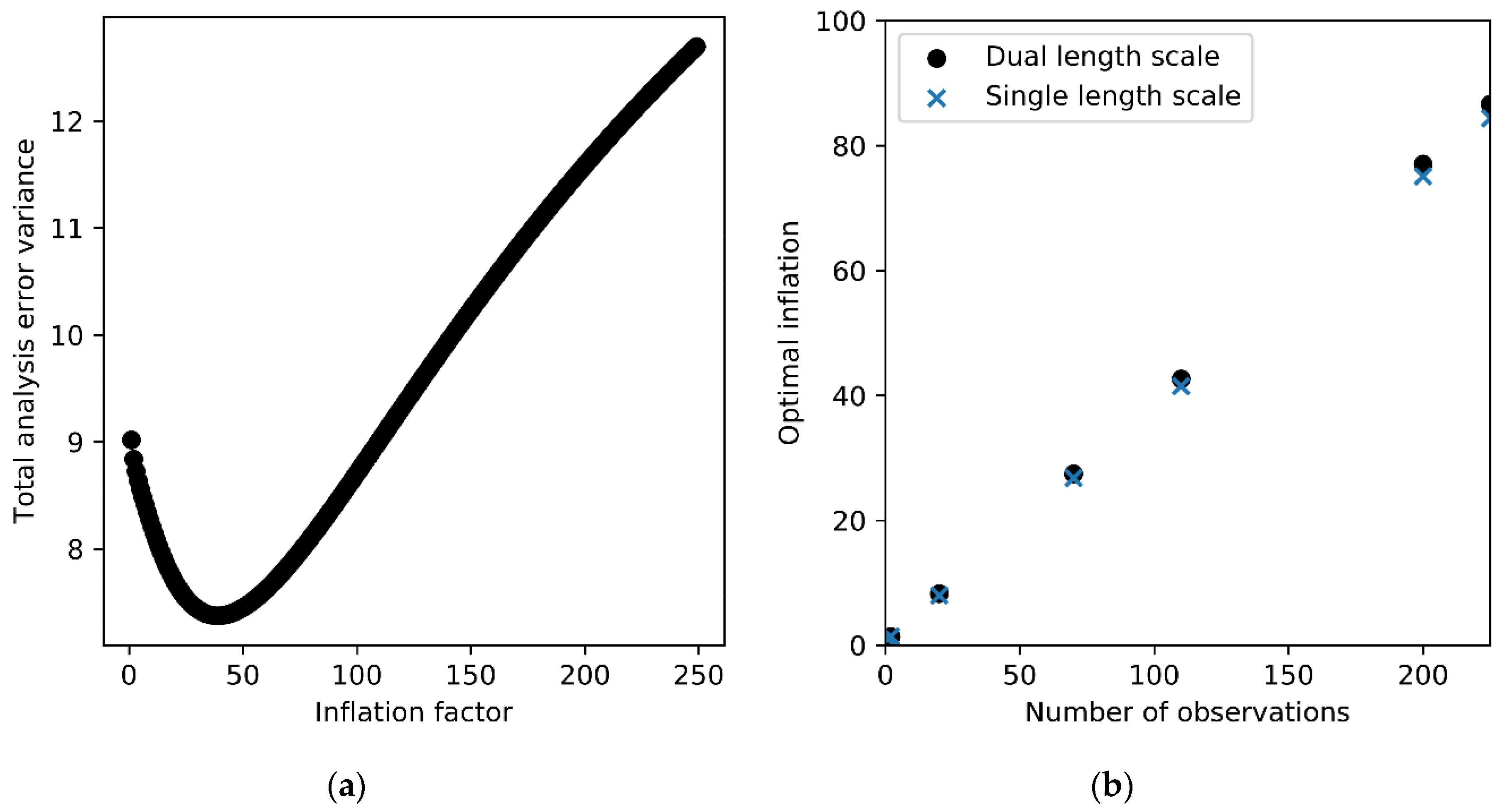
The other main result from the idealised test was that the optimal inflation increases linearly with the number of nearby observations. To be able to apply this concept practically in OSTIA, we define for each observation the ‘observation density’ as the number of other observations from that satellite platform within a radius of 100 km. 100 km, being the length scale of the observation error correlations, was deemed an appropriate way of considering observations to be ‘close’. Tests revealed that the typical maximum ‘observation density’ (by this definition) for each observation type was approximately 1000. In order for the scaling to be coded in a practical way, this was used to define the scaling of the inflation, so that when ‘observation density’ = 1000 the inflation was at its maximum, and when ‘observation density’ = 1 (i.e. no other observations present within 100 km), no inflation is applied.
The results from 
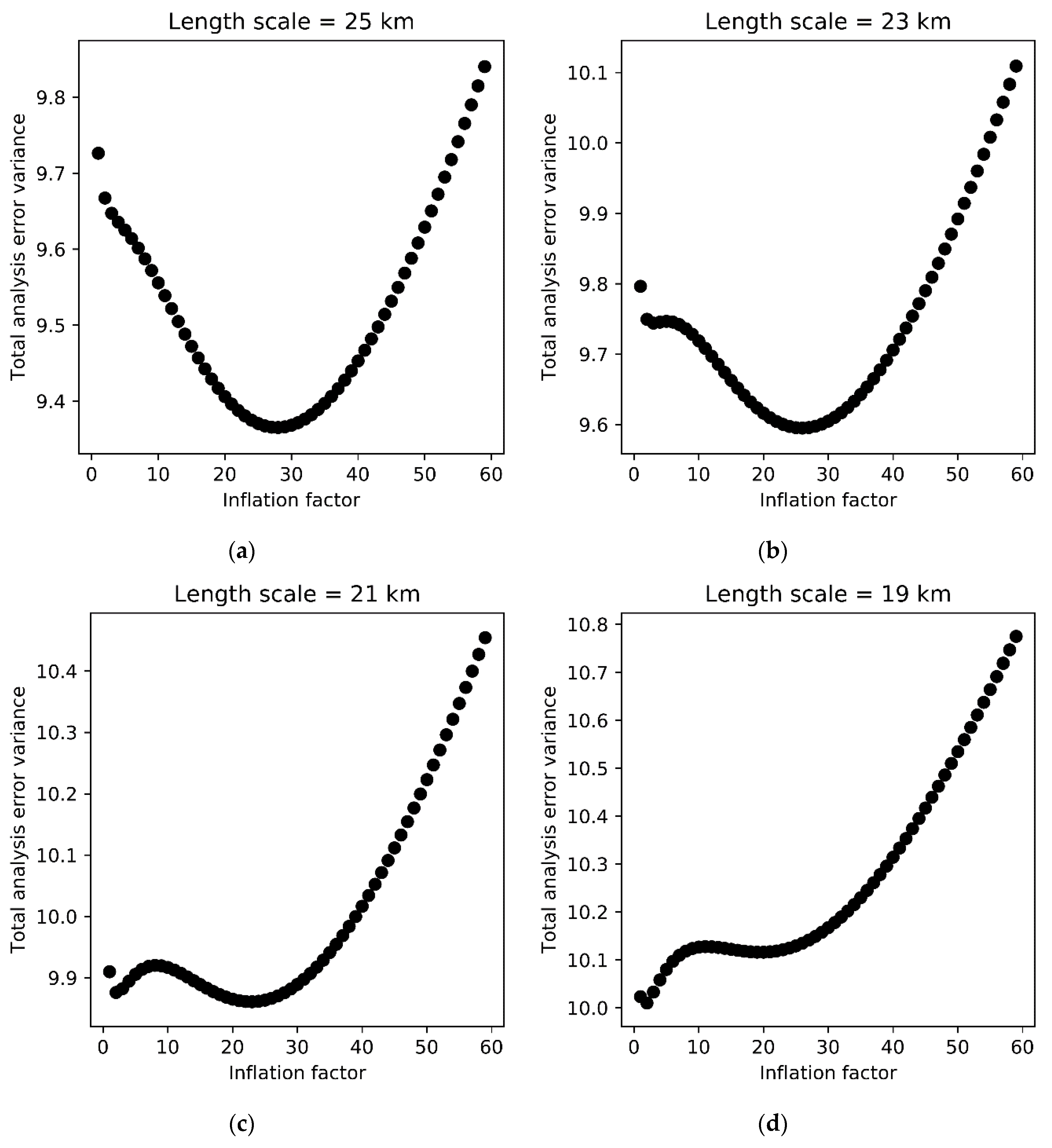
Section 2 clearly show that over-inflating observation error variances can degrade the analysis by a large amount. [18] suggested that an appropriate limit to the inflation factor would be 2–4. A limit of this size is also supported by the results shown in Figure 4. Therefore, a limit of this order should avoid excessive error inflation.
Several OSTIA trials were run for a selected portion of the ESA SST CCI processing described in [5] to investigate the effect of inflating OEVs on the (re)analysis. Each trial was run from January to August 2010, with the first month treated as a spin up period. For this period the available SST CCI observations were from the Advanced Along-Track Scanning Radiometer (AATSR) and the Advanced Very High Resolution Radiometers (AVHRRs) on board the National Oceanic and Atmospheric Administration (NOAA) 17, 18, 19 and MetOp-A platforms.
In the main inflation scheme that was tested (Scheme A), an inflation factor f was applied to OEVs for each satellite as defined in Equations (6)–(8). Inflation was only applied if the ‘ratio condition’ of 0.4 was met.
f = 1  if ratio > 0.4
f = 1 + (m − 1) ρ/ρm  if ratio < 0.36 (i.e., 0.9 × 0.4)
f = 1 + 10 (rc − r) (f* − 1)/rc  if 0.36 ≤ ratio ≤ 0.4
In these equations, r is the ratio (the weighting assigned to the small and large-scale background error covariance components at the observation position), rc is the ratio condition (0.4), ρ is the observation density (defined for each observation as the number of observations within a 100 km radius of itself), ρm is the maximum observation density (1000) above which the maximum inflation is applied, m is the chosen limit to the inflation factor and f* is the f found from Equation (7). The ramping between ratio values of 0.36 and 0.4 is applied in order to avoid a sudden change in OEVs in areas near the boundary of the ratio condition. In summary, the inflation is set to m if the ratio is less than 0.36 and the number of observations within 100 km is at least 1000. The inflation is reduced to 1 as the ratio increases towards 0.4 and number of observations reduces to 1.
An alternative scheme (Scheme B), which did not use the observation density, was also tested. In this scheme, Equation (9) replaces Equation (7).
f = m  if ratio < 0.36 (i.e., 0.9 × 0.4)
Trials were performed as summarised in Table 2. Two sets of trials were defined which were identical except for the observations that were used. In the first set, only AATSR data were used. These trials could give insight into the appropriateness of the inflation methods for a case in which relatively little data are available, for example in an early period. The second set of trials assimilated all available observations, to investigate the more common situation that several observation types are available.
Within each set, control runs were performed in which no inflation was applied, as in the current OSTIA system. There were also cases where the ratio condition was used or not, to evaluate the conclusion from Section 2 that applying inflation everywhere would be detrimental. This is equivalent to assuming the ratio is <0.36 everywhere in Equations (6)–(9). There were also trials aimed at evaluating the use of the observation density to determine inflation (Scheme A compared to Scheme B) and to compare using a maximum inflation of 2, 4, 10 or 50 (note that these are factors applied to the observation error standard deviation).

3.2. Results

3.2.1. Argo Matchups

The outputs from the OSTIA trials were first evaluated by comparing them to Argo data. Matchups to Argo [19] observations from the EN4 database [20] were performed to validate the resulting OSTIA SST fields. Argo observations are not assimilated in OSTIA, so are a valuable independent dataset for validation. Measurements between 3 and 5 m depth have been shown to be representative of foundation SST, but have also been used to evaluate SST CCI L4 outputs [21]. Bilinear interpolation was performed to calculate analysis minus observation statistics for the trial period. This was done for the global ocean and the North Atlantic in the months of June, July and August. This is a region where the ratio condition is met in a significant part in that season, as shown in Figure 5c. This figure also reveals that, in general, the ratio condition is not met in the OSTIA system, i.e., the correlation length scale of the observations errors is sufficiently close to the length scale for the background errors that inflation is unwise.
Results of the Argo matchups are given in Table 3. Differences are very small and hence it is not possible to distinguish between the versions of applying inflation (or not) based on these results. Using AATSR only or all observations does cause a difference in the results, as might be expected. However, the degradation in the standard deviation of differences when using all observations compared to only AATSR is unexpected. It might indicate that there is discrepancy between the AVHRR and AATSR data.
In addition, the control_allobs and infl2_cond_dens_allobs cases were run for the whole of 2010 and global and regional Argo statistics calculated in order to determine if differences would emerge over a longer time period. However, the statistics for the two runs (not shown) contained only minor differences, similar to those seen in the results in Table 3.

3.2.2. Gradients

We now investigate the impact of the inflation method on small-scale features in the analysis since they are expected to be altered [
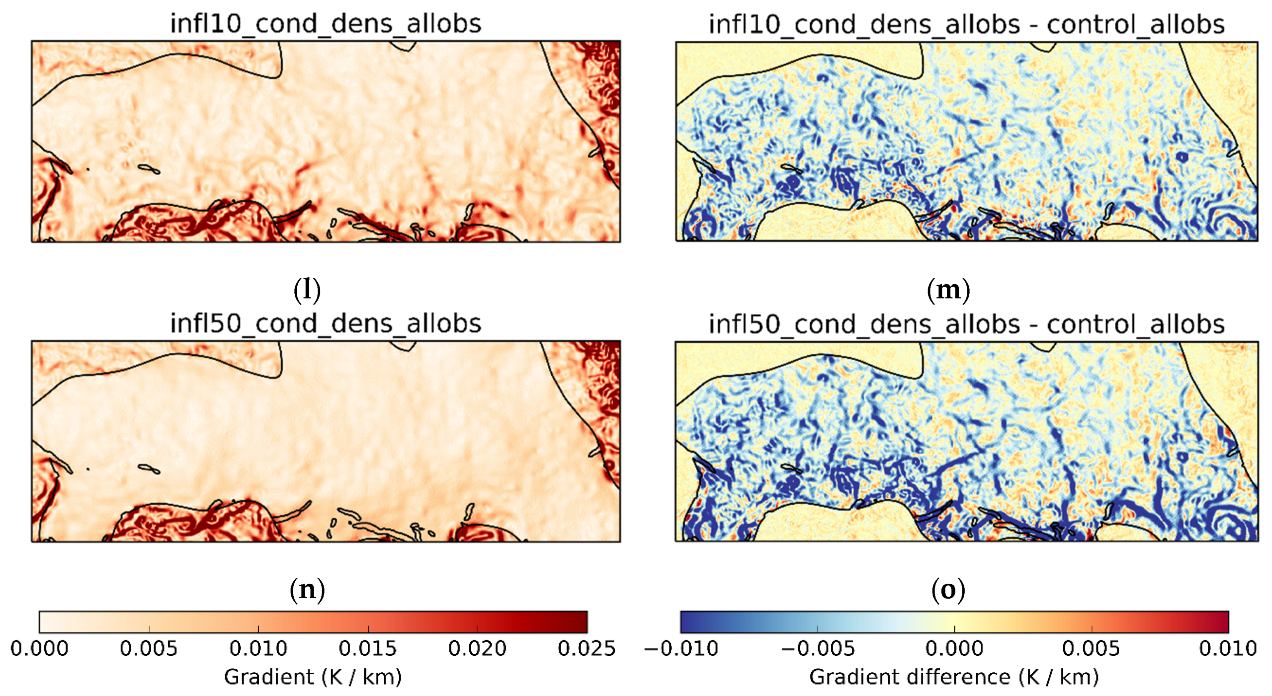
12]. An assimilation that over-fits to observations could result in spurious features in the analysis, so a method that corrects this might be expected to reduce the presence of spurious features. On the other hand, reduced resolution of realistic features in the analyses could point to having under-fitted to observations in the assimilation. Plots of the SST gradients in the region marked by the black box in Figure 5a (−25° to 10° longitude and −30° to −18° latitude) were examined for evidence of these effects. Example outputs are shown in Figure 6. The left column shows an example of the gradients in that region for the cases where all observations were used, and the right column the differences in gradients compared to the control trial. The black contour gives an indication of where the ratio condition is met.
The differences in gradients between the no inflation control case and the case where an inflation factor of 2 is applied everywhere are small, which might suggest that the inflation factor is too low for the quantity of observations that are being assimilated. The case where the density of observations is used to scale the inflation factor has both increases and decreases in gradients compared to the control. This is likely to be because the spreading of observation information spatially has been affected by applying different amounts of inflation in different places. This is particularly evident in the case where inflation has been applied only where the ratio condition is met. Within that region, the gradients are lower than in the case where the inflation was applied everywhere, despite the inflation being the same inside the region. This may be because the observations that are inside the region, which provide the information on small-scale features, are being given less weight in the analysis. Instead, the observations that are outside the region and have not been subjected to inflation have more weight, giving a smoother analysis. However, this requires further investigation. Moving to the case where the density is used to determine inflation where the ratio condition is met largely restores the reduced gradients, but doubling the inflation amount reduces them again. Larger inflation factors further suppress the gradients.

4. Discussion and Conclusions

Correlations in observation errors are generally assumed to be non-existent in L4 SST processing systems such as OSTIA [22]. However, correlations can occur, for example due to retrieval errors. Using information on satellite SST error correlations provided by the ESA SST CCI project, an investigation has been conducted to determine if a commonly used technique to mitigate for these correlations can be improved upon and used in the OSTIA system. This technique involves inflating the observation uncertainties by some amount.
Idealised tests were conducted to determine what the inflation factor should be and how it should be applied. It was found that in some regions the optimal inflation factor varies linearly with the number of observations present. This result could be seen as intuitive—the more observations are present, the greater the effect of ignoring correlated errors, and the higher the inflation needed to counteract the overuse of observations. However, this result was not always applicable to areas where the observation error correlation length scale was less than that for the background errors (known as the ratio condition). Theoretically, applying inflation elsewhere could lead to unpredictable results and a degraded analysis.
The results from the idealised tests were adapted to the OSTIA system and trials run to compare different choices in the inflation algorithm. These were (1) whether the inflation was applied everywhere or only where the observation error correlation length scale was shorter than that for the background errors; (2) whether the inflation should be scaled according to the density of observations; and (3) whether the maximum inflation factor applied to the error standard deviations was 2, 4, 10 or 50. Trials were also run where only AATSR data were assimilated and where all available observations were assimilated and results presented for the globe and for a trial region, which was selected because it mostly met the ratio condition.
The idealised tests indicated that applying inflation, if done correctly, would result in an improvement in the analysis accuracy. However, results from tests comparing the trial data to Argo reference observations were almost identical between all the different trials suggesting no significant advantage or disadvantage to applying the inflation, and no difference whether it was applied everywhere or only where it was thought to be beneficial. This was consistent whether only AATSR was in use or all observations.
Comparison of SST gradients in an example region showed that the choice of inflation algorithm does have an impact on the smoothness of the analysis. The largest impacts were seen when differential inflation was applied, i.e., where the density of observations or the ratio condition was used to control the inflation factor. The greatest impact was seen when only the ratio condition was used as it was found that the analysis became much smoother within the region where the condition applies. This is hypothesised to be because the analysis in those locations was giving extra weight to the observations outside the region where the ratio condition was met rather than the local observations which contain the information on small-scale features. If this is the case, a larger ramping region where the inflation factors are scaled to avoid a ‘shock’ to the analysis system may be beneficial. However, using the density factor and the ratio condition together was found to have a less detrimental impact on the gradients.
These results indicate that, in theory, the inflation method should be beneficial to the OSTIA system and SST analysis systems in general. However, the practical implementation is challenging. Improved understanding of the background and observation error covariances would be the key to applying the method in a broader way than was done in the case studies presented here. For example, the idealised test condition plays a large role in the experiments undertaken, but is based on several assumptions, including that the observation error correlations can be approximated by a Gaussian. This points to the importance of determining the length scale and distribution of the synoptic scale observation error correlations more accurately, for example using techniques such as described by [23]. Another assumption made is that cross-platform observation error correlations are negligible. However, one source of error correlations is the presence of weather systems, whose effect on different platforms may well be correlated. It would be important to determine these correlations, if and where they exist.
Finally, these results point to needing more sophisticated data assimilation methods in the long term, which would allow observation error correlation information to be fully used within analysis systems such as OSTIA.

Author Contributions

Formal analysis, R.R. and S.G.; Methodology, R.R., S.G. and M.J.M.; Software, R.R. and S.G.; Supervision, S.G. and M.J.M.; Visualization, R.R. and S.G.; Writing—original draft, R.R. and S.G.; Writing—review & editing, S.G. and M.J.M. All authors have read and agreed to the published version of the manuscript.

Funding

This work was funded by the ESA as part of the SST CCI Phase 2 project (4000109848/13/I-NB).

Acknowledgments

The authors thank Chris Merchant for his inputs during the study and review of the draft manuscript. We thank the three reviewers and academic editor for their comments, which helped to improve the manuscript. Argo data were collected and made freely available by the International Argo Program and the national programs that contribute to it. (http://www.argo.ucsd.edu, http://argo.jcommops.org). The Argo Program is part of the Global Ocean Observing System.

Conflicts of Interest

The authors declare no conflict of interest. The funders reviewed the work and encouraged its publication.

References

  1. Good, S.A.; Rayner, N. ESA SST CCI Phase 1 User Requirements Document. 2010. Available online: http://www.esa-sst-cci.org/PUG/documents.htm (accessed on 16 March 2020).
  2. Donlon, C.J.; Martin, M.; Stark, J.; Roberts-Jones, J.; Fiedler, E.; Wimmer, W. The Operational Sea Surface Temperature and Sea Ice Analysis (OSTIA) system. Remote Sens. Environ. 2012, 116, 140–158. [Google Scholar] [CrossRef]
  3. Good, S.; Fiedler, E.; Mao, C.; Martin, M.J.; Maycock, A.; Reid, R.; Roberts-Jones, J.; Searle, T.; Waters, J.; While, J.; et al. The Current Configuration of the OSTIA System for Operational Production of Foundation Sea Surface Temperature and Ice Concentration Analyses. Remote Sens. 2020, 12, 720. [Google Scholar] [CrossRef] [Green Version]
  4. Merchant, C.J.; Embury, O.; Roberts-Jones, J.; Fiedler, E.; Bulgin, C.E.; Corlett, G.K.; Good, S.; McLaren, A.; Rayner, N.; Morak-Bozzo, S.; et al. Sea surface temperature datasets for climate applications from Phase 1 of the European Space Agency Climate Change Initiative (SST CCI). Geosci. Data J. 2014, 1, 179–191. [Google Scholar] [CrossRef] [Green Version]
  5. Merchant, C.J.; Embury, O.; Bulgin, C.E.; Block, T.; Corlett, G.K.; Fiedler, E.; Good, S.A.; Mittaz, J.; Rayner, N.A.; Berry, D.; et al. Satellite-based time-series of sea-surface temperature since 1981 for climate applications. Sci. Data 2019, 6, 223. [Google Scholar] [CrossRef] [PubMed] [Green Version]
  6. Waters, J.; Lea, D.J.; Martin, M.J.; Mirouze, I.; Weaver, A.; While, J. Implementing a variational data assimilation system in an operational 1/4 degree global ocean model. Q. J. R. Meteorol. Soc. 2015, 141, 333–349. [Google Scholar] [CrossRef]
  7. Fiedler, E.K.; Mao, C.; Good, S.A.; Waters, J.; Martin, M.J. Improvements to feature resolution in the OSTIA sea surface temperature analysis using the NEMOVAR assimilation scheme. Q. J. R. Meteorol. Soc. 2019, 145, 3609–3625. [Google Scholar] [CrossRef]
  8. Roberts-Jones, J.; Bovis, K.; Martin, M.J.; McLaren, A. Estimating background error covariance parameters and assessing their impact in the OSTIA system. Remote Sens. Environ. 2016, 176, 117–138. [Google Scholar] [CrossRef]
  9. Bulgin, C.E.O.; Embury, O.; Corlett, G.; Merchant, C.J. Independent uncertainty estimates for coefficient based sea surface temperature retrieval from the Along-Track Scanning Radiometer instruments. Remote Sens. Environ. 2016, 178, 213–222. [Google Scholar] [CrossRef] [Green Version]
  10. Oke, P.R.; Sakov, P. Representation Error of Oceanic Observations for Data Assimilation. J. Atmos. Oceanic Technol. 2008, 25, 1004–1017. [Google Scholar] [CrossRef] [Green Version]
  11. Janjić, T.; Bormann, N.; Bocquet, M.; Carton, J.A.; Cohn, S.E.; Dance, S.L.; Losa, S.N.; Nichols, N.K.; Potthast, R.; Waller, J.A.; et al. On the representation error in data assimilation. Q. J. R. Meteorol. Soc. 2018, 144, 257–1278. [Google Scholar] [CrossRef]
  12. Rainwater, S.; Bishop, C.H.; Campbell, W.F. The benefits of correlated observation errors for small scales. Q. J. R. Meteorol. Soc. 2015, 141, 3439–3445. [Google Scholar] [CrossRef]
  13. Liu, Z.; Rabier, F. The potential of high-density observations for numerical weather prediction: A study with simulated observations. Q. J. R. Meteorol. Soc. 2003, 129, 3013–3035. [Google Scholar] [CrossRef]
  14. Miyoshi, T.; Kalnay, E.; Li, H. Estimating and including observation-error correlations in data assimilation. Inverse Probl. Sci. Eng. 2013, 21, 387–398. [Google Scholar] [CrossRef]
  15. Fowler, A.M.; Dance, S.L.; Waller, J.A. On the interaction of observation and prior error correlations in data assimilation. Q. J. R. Meteorol. Soc. 2018, 144, 48–62. [Google Scholar] [CrossRef] [Green Version]
  16. Hoffman, R.N. The Effect of Thinning and Superobservations in a Simple One-Dimensional Data Analysis with Mischaracterized Error. Mon. Wea. Rev. 2018, 146, 1181–1195. [Google Scholar] [CrossRef]
  17. Mirouze, I.; Weaver, A.T. Representation of correlation functions in variational assimilation using an implicit diffusion operator. Q. J. R. Meteorol. Soc. 2010, 136, 1421–1443. [Google Scholar] [CrossRef]
  18. Stewart, L.M.; Dance, S.L.; Nichols, N.K. Data assimilation with correlated observation errors: Experiments with a 1-D shallow water model. Tellus A Dyn. Meteorol. Oceanogr. 2013, 65, 1. [Google Scholar] [CrossRef]
  19. Argo. Argo float data and metadata from Global Data Assembly Centre (Argo GDAC). SEANOE 2020. [Google Scholar] [CrossRef]
  20. Good, S.A.; Martin, M.J.; Rayner, N.A. EN4: Quality controlled ocean temperature and salinity profiles and monthly objective analyses with uncertainty estimates. J. Geophys. Res. Oceans 2013, 118, 6704–6716. [Google Scholar] [CrossRef]
  21. Fiedler, E.K.; McLaren, A.; Banzon, V.; Brasnett, B.; Ishizaki, S.; Kennedy, J.; Rayner, N.; Roberts-Jones, J.; Corlett, G.; Merchant, C.J.; et al. Intercomparison of long-term sea surface temperature analyses using the GHRSST Multi-Product Ensemble (GMPE) system. Remote Sens. Environ. 2019, 222, 18–33. [Google Scholar] [CrossRef] [Green Version]
  22. Martin, M.; Dash, P.; Ignatov, A.; Banzon, V.; Beggs, H.; Brasnett, B.; Cayula, J.F.; Cummings, J.; Donlon, C.; Gentemann, C.; et al. Group for High Resolution Sea Surface temperature (GHRSST) analysis fields inter-comparisons. Part 1: A GHRSST multi-product ensemble (GMPE). Deep Sea Res. Part II Top. Stud. Oceanogr. 2012, 77–80, 21–30. [Google Scholar] [CrossRef]
  23. Waller, J.A.; Dance, S.L.; Nichols, N.K. Theoretical insight into diagnosing observation error correlations using observation-minus-background and observation-minus-analysis statistics. Q. J. R. Meteorol. Soc. 2016, 142, 418–431. [Google Scholar] [CrossRef] [Green Version]
Figure 1. (a) Example plot to demonstrate the diagnosis of the optimal inflation factor showing inflation factor against resulting analysis error variance for the Western Central Pacific case with 100 observations. (b) Optimal observation error variance inflation, calculated in the Western Central Pacific case, for varying numbers of observations and using either a dual length scale or a single length scale to represent the background error correlations.
Remotesensing 12 01083 g001
Figure 2. As Figure 1, but showing results for the North-West Pacific region.
Remotesensing 12 01083 g002
Figure 3. Analysis error variance for varying inflation factors for identical conditions apart from a small change in the length scale associated with errors correlated on small scales. (a) Length scale set to 25 km; (b) length scale set to 23 km; (c) length scale set to 21 km; and (d) length scale set to 19 km.
Remotesensing 12 01083 g003
Figure 4. Impact on the optimal inflation from varying (a) the background error correlation length scale for the Western Central Pacific (WCP) and North-West Pacific (NWP) regions; (b) the background and observation error variances for the WCP. The crosses show the values of the parameters being varied in the original set up.
Remotesensing 12 01083 g004
Figure 5. (a) Example from the Dec-Feb season of the ratios used in the OSTIA system to determine the relative weighting of the small and large-scale covariance components. The blue contour shows where the ratio is 0.4 and the black box indicates an example region, within which the ratio condition is generally met. (b) Mar-May season; (c) Jun-Aug season; (d) Sep-Nov season.
Remotesensing 12 01083 g005
Figure 6. (a,b,d,f,h,j,l,n) horizontal SST gradients between −25° to 10° longitude and −30° to −18° latitude on 19 February, 2010, from each of the trials where all the observations were in use. (c,e,g,i,k,m,o) differences between the control_allobs trial and the other trials.
Remotesensing 12 01083 g006aRemotesensing 12 01083 g006b
Table 1. Regions modelled in the idealised tests.
Area NameObservation Synoptic Error Variance (K2)Observation Synoptic Error Correlation Length Scale (km)Background Small-Scale Error Variance (K2)Background Small-Scale Error Correlation Length Scale (km)Background Large-Scale Error Variance (K2)Background Large-Scale Error Correlation Length Scale (km)
North West Pacific0.141000.7250.35250
West Central Pacific0.041000.05700.05700
North East Pacific0.041000.05250.05250
Table 2. Configuration of Operational Sea Surface Temperature and Ice Analysis (OSTIA) trials.
Name of TrialObservations AssimilatedInflation Applied Everywhere or Within Ratio ConditionInflation Scheme Applied to OEVsMaximum Inflation Factor
control_aatsrAATSR onlyN/ANone1
infl2_all_aatsrAATSR onlyEverywhereB2
infl2_all_dens_aatsrAATSR onlyEverywhereA2
infl2_cond_aatsrAATSR_onlyWithin conditionB2
infl2_cond_dens_aatsrAATSR onlyWithin conditionA2
infl4_cond_dens_aatsrAATSR onlyWithin conditionA4
control_allobsAllN/ANone1
infl2_all_allobsAllEverywhereB2
infl2_all_dens_allobsAllEverywhereA2
infl2_cond_allobsAllWithin conditionB2
infl2_cond_dens_allobsAllWithin conditionA2
infl4_cond_dens_allobsAllWithin conditionA4
infl10_cond_dens_allobsAllWithin conditionA10
infl50_cond_dens_allobsAllWithin conditionA50
Table 3. Statistics from comparing Argo reference data to the outputs from the OSTIA trials.
StatisticTrialGlobeNorth Atlantic
Mean of differences (analysis minus Argo) (K)control_aatsr−0.0440.000
infl2_all_aatsr−0.0420.003
infl2_all_dens_aatsr−0.047−0.002
infl2_cond_aatsr−0.0430.000
infl2_cond_dens_aatsr−0.0440.000
infl4_cond_dens_aatsr−0.0440.000
control_allobs−0.060−0.022
infl2_all_allobs−0.059−0.021
infl2_all_dens_allobs−0.061−0.021
infl2_cond_allobs−0.060−0.020
infl2_cond_dens_allobs−0.060−0.021
infl4_cond_dens_allobs−0.060−0.019
infl10_cond_dens_allobs−0.059−0.015
infl50_cond_dens_allobs−0.058−0.012
Standard deviation of differences (K)control_aatsr0.5510.653
infl2_all_aatsr0.5490.648
infl2_all_dens_aatsr0.5520.657
infl2_cond_aatsr0.5510.654
infl2_cond_dens_aatsr0.5520.654
infl4_cond_dens_aatsr0.5510.654
control_allobs0.5250.612
infl2_all_allobs0.5220.607
infl2_all_dens_allobs0.5250.610
infl2_cond_allobs0.5240.609
infl2_cond_dens_allobs0.5250.611
infl4_cond_dens_allobs0.5250.610
infl10_cond_dens_allobs0.5240.609
infl50_cond_dens_allobs0.5240.608
Number of observationsAll trials171152522

