Article

Deep Relation Network for Hyperspectral Image Few-Shot Classification

1
Information Engineering University, Zhengzhou 450001, China
2
Xi’an Research Institute of Surveying and Mapping, Xi’an 710054, China
*
Author to whom correspondence should be addressed.
Remote Sens. 2020, 12(6), 923; https://doi.org/10.3390/rs12060923
Submission received: 20 February 2020 / Revised: 8 March 2020 / Accepted: 10 March 2020 / Published: 13 March 2020
(This article belongs to the Special Issue Advances in Hyperspectral Data Exploitation)

Abstract

:
Deep learning has achieved great success in hyperspectral image classification. However, when processing new hyperspectral images, the existing deep learning models must be retrained from scratch with sufficient samples, which is inefficient and undesirable in practical tasks. This paper aims to explore how to accurately classify new hyperspectral images with only a few labeled samples, i.e., the hyperspectral images few-shot classification. Specifically, we design a new deep classification model based on relational network and train it with the idea of meta-learning. Firstly, the feature learning module and the relation learning module of the model can make full use of the spatial–spectral information in hyperspectral images and carry out relation learning by comparing the similarity between samples. Secondly, the task-based learning strategy can enable the model to continuously enhance its ability to learn how to learn with a large number of tasks randomly generated from different data sets. Benefitting from the above two points, the proposed method has excellent generalization ability and can obtain satisfactory classification results with only a few labeled samples. In order to verify the performance of the proposed method, experiments were carried out on three public data sets. The results indicate that the proposed method can achieve better classification results than the traditional semisupervised support vector machine and semisupervised deep learning models.

Graphical Abstract

1. Introduction

Hyperspectral remote sensing, as an important means of earth observation, is one of the most important technological advances in the field of remote sensing. Utilizing the imaging spectrometer with very high spectral resolution, hyperspectral remote sensing can obtain abundant spectral information on the observation area so as to produce hyperspectral images (HSI) with a three-dimensional data structure. As HSI have the unique advantage of “spatial–spectral unity” (HSI contain both abundant spectral and spatial information), hyperspectral remote sensing has been widely used in fine agriculture, land-use planning, target detection, and many other fields.
HSI classification is one of the most important steps in HSI analysis and application, the basic task of which is to determine a unique category for each pixel. In early research, the working mode of feature extraction combined with classifiers such as support vector machines (SVM) [1] and random forest (RF) [2] was dominant at the time. Initially, in order to alleviate the Hughes phenomenon caused by band redundancy, researchers introduced a series of feature extraction methods to extract spectral features conducive to classification from abundant spectral information. Common spectral feature extraction methods include principal component analysis (PCA) [3], independent component analysis (ICA) [4], linear discriminant analysis (LDA) [5], and other linear methods, as well as kernel principal component analysis (KPCA) [6], locally linear embedding (LLE) [7], t-distributed stochastic neighbor embedding (t-SNE) [8], and other nonlinear methods. Admittedly, the above feature extraction method can achieve some results, but ignoring spatial structure information in HSI still seriously hinders the increase of classification accuracy. To this end, a series of spatial information utilization methods are introduced, such as extended morphological profile (EMP) [9], local binary patterns (LBP) [10], 3D Gabor features [11], Markov random field (MRF) [12], spatial filtering [13], variants of non-negative matrix underapproximation (NMU) [14], and so on. The extraction and utilization of spatial features can effectively improve classification accuracy. However, due to the separation of feature extraction process and classification in traditional classification mode, the adaptability between them cannot be fully considered [15]. In addition, the classification results of traditional methods largely depend on the accumulated experience and parameter setting, which lacks stability and robustness.
In recent years, with the development of artificial intelligence, deep learning has been applied to the field of remote sensing [16]. Compared to traditional methods, deep learning can automatically learn the required features from the data by establishing a hierarchical framework. Moreover, these features are often more discriminative and more conducive to the classification. Stacked AutoEncoder (SAE) [17], recurrent neural network (RNN) [18,19], and deep belief networks (DBN) [20,21] are first applied to HSI classification. These methods can achieve higher classification accuracy than traditional methods under certain conditions. Nevertheless, some necessary preprocessing must be performed to transform HSI into a one-dimensional vector for feature extraction, which destroys the spatial structure information in HSI. Compared with the above deep learning models, convolutional neural networks (CNNs) are more suitable for HSI processing and feature extraction. At present, 2D-CNN and 3D-CNN are two basic models widely used in HSI classification [22]. By means of two-dimensional and three-dimensional convolution operation, 2D-CNN and 3D-CNN can both fully extract and utilize the spatial–spectral features in HSI. Yue et al. take the lead in exploring the effect of 2D-CNN in HSI classification. Subsequently, many improved models based on 2D-CNN have been proposed and refresh classification accuracy constantly, such as DR-CNN [23], contextual deep CNN [24], DCNN [25], DC-CNN [26], and so on. Most 2D-CNN-based methods use PCA to reduce the dimension of HSI in order to reduce the number of channels in the convolution operation. However, this practice inevitably loses important detail information in HSI. The advantage of 3D-CNN is that it can directly perform three-dimensional convolution operation on HSI without any preprocessing and can make full use of spatial–spectral information to further improve classification accuracy. Chen et al. take the lead in utilizing 3D-CNN for HSI classification and have conducted detailed studies on the number of network layers, number of convolution kernels, size of the neighborhood, and other hyperparameters [27]. On this basis, methods such as residual learning [28], attention mechanism [29], dense network [30], and multiscale convolution [31] are combined with 3D-CNN, resulting in higher classification accuracy. In addition, CNN is combined with other methods such as active learning [32], capsule network [33], superpixel segmentation [34], and so on, which can achieve promising classification results when the training samples are sufficient.
Indeed, deep learning has seen great success in HSI classification. However, there is still a serious contradiction between the huge parameter space of the deep learning model and the limited labeled samples of HSI. In other words, the deep learning model must have enough labeled samples as a guarantee, so as to give full play to the its classification performance. Nevertheless, it is difficult to obtain enough labeled samples in practice, because the acquisition of labeled samples is time-consuming and laborious. In order to improve classification accuracy under the condition of limited labeled samples, semisupervised learning and data augmentation are widely applied. In [35,36], CNN was combined with semisupervised classification. In [37], Kang et al. first extracted PCA, EMP, and edge-preserving features (EPF), then carried out classification by combining semisupervised method and decision confusion strategy. In [27], Chen et al. generated virtual training samples by adding noise to the original labeled samples, while in [38,39], the number of training samples were increased by constructing training sample pairs. In recent years, with the emergence of generative adversarial networks (GANs), many researchers have utilized the synthetic sample generated by GAN to assist in training networks [40,41,42]. It is true that the above methods can improve classification accuracy under the condition of limited labeled samples, but they either further explore the feature of the insufficient labeled samples or utilize the information of unlabeled samples in the HSI being classified to further train the model. In other words, the HSI used to train model are exactly identical to the target HSI used to test the model. This means that when processing a new HSI, the model must be retrained from scratch. However, it is impossible to train a classifier for each HSI, which will incur significant overhead in practice.
Few-shot learning is when a model can effectively distinguish the categories in the new data set with only a very few labeled samples processing a new data set [43]. The availability of very few samples challenges the standard training practice in deep learning [44]. Different from the existing deep learning model, however, humans are very good at few-shot learning, because they can effectively utilize the previous learning experience and have the ability to learn how to learn, which is the concept of meta-learning [45,46]. Therefore, we should effectively utilize transferable knowledge in the collected HSI to further classify other new HSI, so as to reduce cost as much as possible. Different HSI contain different types and quantities of ground objects, so it is difficult for the general transfer learning [47,48] to obtain satisfactory classification accuracy with a few labeled sample. According to the idea of meta-learning, the model not only needs to learn transferable knowledge that is conducive to classification but also needs to learn the ability to learn.
The purpose of this paper is to explore how to accurately classify new HSI which are absolutely different from the HSI used for training with only a few labeled samples (e.g., five labeled samples per class). More specifically, this paper designs a new model based on a relation network [49] for HSI few-shot classification (RN-FSC) and trains it with the idea of meta-learning. The designed model is an end-to-end framework, including two modules: feature learning module and relation learning module, which can effectively simplify the classification process. The feature learning module is responsible for extracting deep features from samples in HSI, while the relation learning module carries on relation learning by comparing the similarity between different samples, that is, the relation score between samples belonging to the same class is high, and the relation score between samples belonging to different class is low. From the perspective of workflow, the proposed RN-FSC method consists of three steps. In the first step, we use the designed network model to carry out meta-learning on the source HSI data set, so that the model can fully learn the transferable feature knowledge and relation comparison ability, i.e., the ability to learn how to learn. In the second step, the network model is fine-tuned with only a few labeled samples in the target HSI data set so that the model can quickly adapt to new classification scenarios. In the third step, the target HSI data sets are used to test the classification performance of the proposed method. It is important to note that the target HSI data set for classification and the source HSI data set for meta-learning are completely different.
The main contributions of this paper are as follows:
  • The RN-FSC method is proposed to carry out classification on the new HSI with only a few labeled samples. The RN-FSC method has the ability to learn how to learn through meta-learning on the source HSI data set, so it can accurately classify the new HSI;
  • The network model containing the feature learning module and relation learning module is designed for HSI classification. Specifically, 3D convolution is utilized for feature extraction to make full use of spatial–spectral information in HSI, and the 2D convolution layer and fully connected layer are utilized to approximate the relationship between sample features in an abstract nonlinear approach;
  • Experiments are conducted on three well-known HSI data sets, which demonstrate that the proposed method can outperform conventional semisupervised methods and the semisupervised deep learning model with a few labeled samples.
The remainder of this paper is structured as follows. In Section 2, HSI few-shot classification is introduced. In Section 3, the design relation network model is described in detail. In Section 4, experimental results and analysis on three public available HSI data sets are presented. Finally, conclusions are provided in Section 5.

2. HSI Few-Shot Classification

In this section, we first explain the definition of few-shot classification, then describe the task-based learning strategy in detail, and finally give the complete process of HSI few-shot classification.

2.1. Definition of Few-Shot Classification

In order to explain the definition of few-shot classification, we must first distinguish several concepts: source data set, target data set, fine-tuning data set, and testing data set. Both the fine-tuning data set and the testing data set are subsets of the target data set, sharing the same label space, while the source data set and the target data set are totally different. With reference to most of the existing deep learning models, we can only utilize the fine-tuning data set to train a classifier. However, the classification performance of this classifier is very poor due to the very small fine-tuning data set. Therefore, we need to use the idea of meta-learning to carry out the classification task (as shown in Figure 1). The model first performs meta-learning on the source data set to extract the transferable feature knowledge and cultivate the ability of learning to learn. After meta-learning, the model can acquire enough generalization knowledge. Then, the model is fine-tuned on the fine-tuning data set to extract individual knowledge, so as to adapt to the new classification scenario quickly. The fine-tuning data set is very small compared to the testing data set, so the process of fine-tuning can be called few-shot learning. If the fine-tuning data set contains C unique classes and each class includes K labeled samples, the classification problem can be called C-way K-shot. Finally, the model is utilized to classify the testing data set.

2.2. Task-Based Learning Strategy

At present, batch-based training strategy is widely used in deep learning models, as shown in Figure 2a. In the training process, each batch contains a certain amount of samples with specific labels. The training process of the model is actually based on samples to calculate the loss and update the network parameters. General transfer learning also uses this strategy for model training.
Meta-learning can also be regarded as a learning process of transferring feature knowledge. The key of meta-learning allowing the model to acquire more outstanding learning ability than general transfer learning is the task-based learning strategy. In meta-learning, tasks are treated as the basic unit for training [45,49]. As shown in Figure 2b, a task contains a support set and a query set. The support set and the query set are sampled randomly from the same data set and share the same label space. The sample x in the support set are clearly labeled by y, while the labels of samples in the query set are regarded as unknown. The model predicts the labels of samples in the query set under the supervision of the support set and calculates the loss by comparing the predictive labels with the real labels, thus realizing the update of parameters.
The model runs on the basis of the task-based learning strategy, whether in the meta-learning phase, the few-shot learning phase, or the classification phase. One task is actually a training iteration. Take meta-learning on a source data set containing C s r c classes as an example. During each iteration, a task is generated by randomly selecting C classes and K samples per class from the source data set. Thus, the support set can be denoted as S = { ( x i , y i ) } i = 1 C × K . Similarly, C × N samples are randomly sampled from the same C classes to form a query set Q = { ( x j , y j ) } j = 1 C × N . It is important to note that there is no intersection between S and Q . In practice, we usually set C < C s r c , which can guarantee the richness of tasks and thus improve the robustness of the model. In theory, N tends to be much larger than K, so as to mimic the actual few-shot classification scenario. In summary, through the above description, a C-way K-shot N-query learning task has been builded on the source data set.

2.3. HSI Few-Shot Classification

In the previous sections, we explained in detail the few-shot classification and its learning strategy. It is not difficult to apply it to HSI classification. We only need to utilize the collected HSI as the source data set, e.g., the Botswana and Houston data sets, and utilize other HSI as the target data set, e.g., the Pavia Center data set. The complete HSI few-shot classification process based on the task-based learning strategy can be summarized as follows.
(1)
In the first phase, learning tasks are built on the source data set, and the model performs meta-learning;
(2)
In the second phase, learning tasks are built on the fine-tuning data set, and the model performs few-shot learning;
(3)
In the third phase, the entire fine-tuning data set is regarded as the support set, and the testing data set is regarded as the query set, so as to build tasks for HSI classification.

3. The Designed Relation Network Model
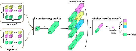
This section introduces the designed relation network model for the HSI few-shot classification. The designed model consists of two core modules, feature learning module and relation learning module, which are introduced in detail. In addition, we explain how the model acquires the ability to learn how to learn from three different perspectives.

3.1. Model Overview

The designed relation network model for HSI few-shot classification consists of three parts: feature learning, feature concatenation, and relation learning, as illustrated in Figure 3. The model is an end-to-end framework, with tasks as inputs and predictive labels as outputs.
Specifically, we select the data cubes belonging to each pixel in HSI as the samples in the task. As defined in Section 2.2, the sample in the support set is denoted as x i , and the sample in the query set is denoted as x j . The feature learning module is equivalent to a nonlinear embedding function f, which maps samples x i and x j in the data space to abstract features f ( x i ) and f ( x j ) in the feature space. Then, features f ( x i ) and f ( x j ) are concatenated in the depth dimension, which can be denoted as C ( f ( x i ) , f ( x j ) ) . Of course, there is more than one way to perform concatenation. It should be noted, however, that each sample feature in the query set should be concatenated to each feature generated by the support set. In addition, in order to simplify the following calculation and improve the robustness of the model, the sample features belonging to the same class in the support set are averaged. Consequently, the number of features generated from the support set is always equal to C. This means that, for the support set S = { ( x i , y i ) } i = 1 C × K and the query set Q = { ( x j , y j ) } j = 1 C × N , C × C × K concatenations would be generated. The relation learning module can also be regarded as a nonlinear function g, which maps each concatenation to a relation score r i , j = g [ C ( f ( x i ) , f ( x j ) ) ] representing the similarity between x i and x j . If samples x i and x j belong to the same class, the relation score will be close to 1, otherwise the relation score will be close to 0. Finally, the maximum score is obtained from the relation score set R = { r l , j } ( l = 1 , , C ) of sample x j , so as to decide the predictive label.
The model is trained with mean square error (MSE) as loss function (Equation (1)). MSE is easy to calculation and sufficient for training. If y i and y j belong to the same class, ( y i = = y j ) is 1, otherwise 0, which can effectively achieve relation learning.
L M S E = i = 1 C × K j = 1 C × N ( r i , j 1 · ( y i = = y j ) ) 2 .

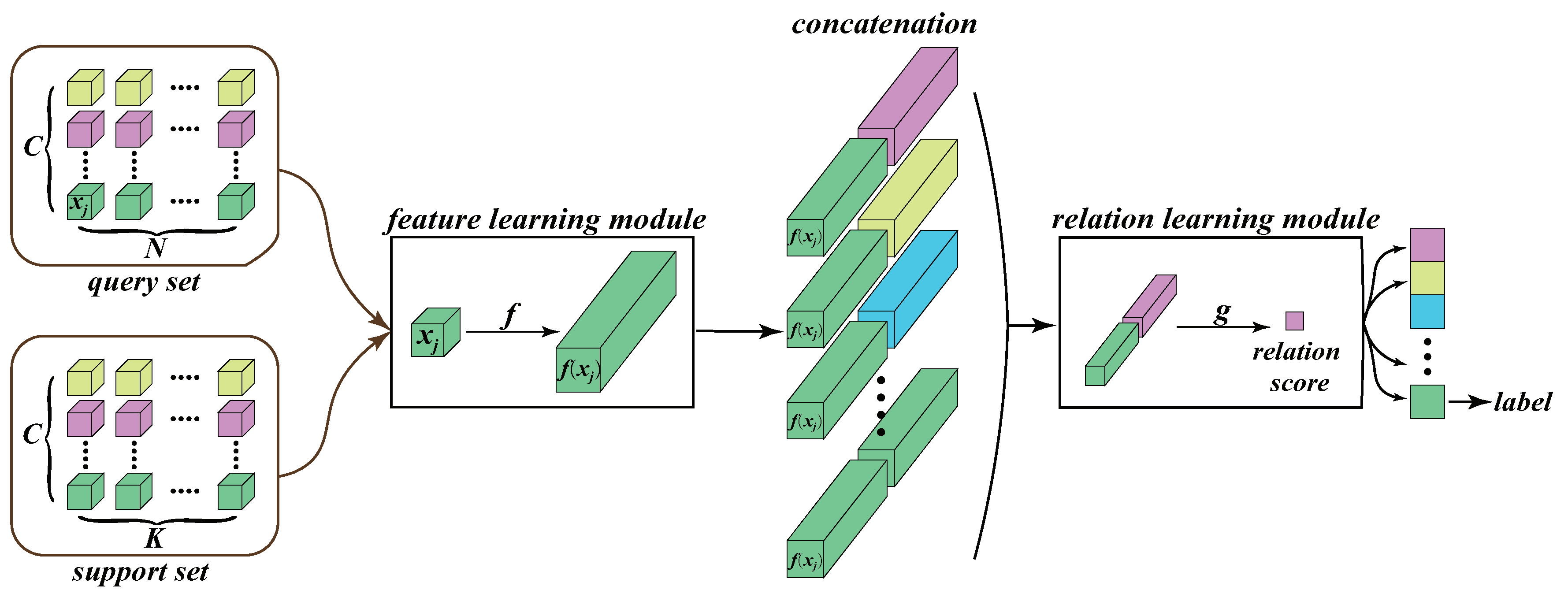
3.2. The Feature Learning Module

The goal of the feature learning module is to extract more discriminative features from the input data cubes. Theoretically, any network structure can be built in this module for feature learning. A large number of studies have shown that 3D convolution is more suitable for the spatial–spectral features extraction because of the close correlation between the spatial domain and spectral domain in HSI. Therefore, we take the 3D convolutional layer as the core and construct the feature learning network as shown in Figure 4.
The feature learning module consists of a 3D convolutional layer, batch normalization layer, Relu activation function, maximum pooling layer, and concatenation operation. 3D convolution can process the input data cubes directly without any preprocessing. Compared with the general 2D convolution, 3D convolution can extract more discriminative spatial–spectral features by cascading spectral information of adjacent bands. Specifically, the 3D convolution kernel is set as 3 × 3 × 3 , and the number of convolution kernel increases from 8 to 32 by multiples, which is consistent with the experience in the field of computer vision. Batch normalization layers are added after each 3D convolutional layer, which can effectively alleviate the problem of vanishing gradient and enhance the generalization ability of the model. Relu activation function, one of the most widely used activation functions in deep learning, can increase the nonlinearity of the model and speed up the convergence. The 3D convolutional layer, batch normalization layer, and Relu layer can be considered as a basic unit. Each unit is connected via maximum pooling layer. Considering the characteristics of HSI, the maximum pooling layer is set to 2 × 2 × 4 to deal with spectral redundancy.
After three convolution operations, the input samples become data cubes with 32 channels. To facilitate the subsequent operation in the feature concatenation phase, we first concatenate the 32 data cubes in the channel dimension. Given that the dimension of the data cubes is ( 32 , H , W , D ) , it becomes ( H , W , D × 32 ) after channel concatenation.

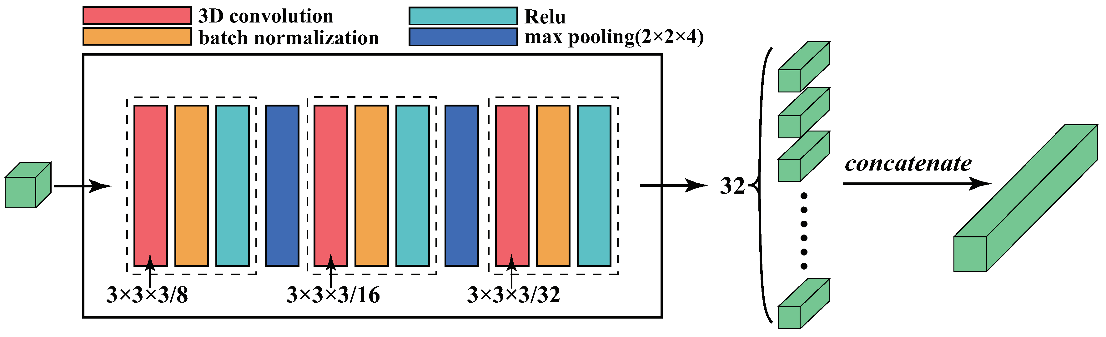
3.3. The Relation Learning Module

Under the combined action of the first two phases, the data cubes are transformed into different concatenations which are the input of the relation learning module (Figure 5). The purpose of the relation learning module is to map each concatenation to a relation score measuring the similarity between the two samples, i.e., the relationship.
In order to speed up computation, 2D convolution is regarded as the core to build the relation learning module. Therefore, the dimension of the concatenations can be regarded as ( H , W , C ) , where C stands for the channel dimension. Considering that the channel dimension is much larger than the spatial dimension, the 1 × 1 2D convolution [50] is first adopted, which can extract the cascaded features across the channel while reducing the dimension effectively. After 1 × 1 convolution, 128 convolution kernels of 3 × 3 are utilized to ensure the diversity of features. In order to fully train the network, the batch normalization layer and Relu activation function are also applied after each convolution. Finally, two fully connected layers of 128 and 1 are added, so as to transform the feature maps into relation scores. Dropout is introduced between the fully connected layer to further enhance the generalization capability. In addition, sigmoid activation function is used to limit the output to the interval [0, 1].
Relation score is not only the final result of relation learning, but also a kind of similarity measure. If the two samples belong to the same class, the relation score is close to 1, otherwise 0. Therefore, the classes of samples in the query set will be determined according to the relation score.

3.4. The Ability of Learning to Learn

Our proposed method, RN-FSC, is essentially a meta-learning-based method for HSI few-shot classification. The core idea of meta-learning is to cultivate the ability of learning to learn. In this section, we expound this ability of RN-FSC from the following three aspects:
(1)
Learning process
General deep learning models are trained based on the unique correspondence between data and labels and can only be trained in one specific task space at a time. However, the proposed method is task-based learning at any phase. The model focuses not on the specific classification task but on the learning ability with many different tasks;
(2)
Scalability
The proposed method performs meta-learning on the source data set to extract the transferable feature knowledge and cultivate the ablitity of learning to learn. From the perspective of knowledge transfer, the richer the categories in the source data set, the stronger the acquired learning ability, which is consistent with the human learning experience. Therefore, we can appropriately extend the source data set to enhance the generalization ability of the model;
(3)
Core mechanism
The proposed method is not to learn how to classify a specific data set, but to learn a deep metric space with the help of many tasks from different data sets, in which relation learning is performed by comparison. In a data-driven way, this metric space is nonlinear and transferrable. By comparing the similarity between the support samples and the query samples in the deep metric space, the classification is realized indirectly.

4. Experiments and Discussion

All experiments were carried out on a laptop with an Intel Core i7-9750H, 2.60 GHz and an Nvidia GeForce RTX 2070. The laptop’s memory is 16 GB. All programs are developed and implemented based on Pytorch library.

4.1. Experimental Data Sets

4.1.1. Source Data Sets

Four publicly available HSI data sets were collected to build the source data sets, which are Houston, Botswana, Kennedy Space Center (KSC), and Chikusei. The four data sets were photographed by different imaging spectrometers on different regions, with different ground sample distance and spectral range (as shown in Table 1). This can ensure the diversity and richness of samples, which is conducive to meta-learning. There are 76 different ground objects contained in the four data sets, and the distribution of their respective labeled samples can be seen in Figure 6, Figure 7, Figure 8 and Figure 9. We exclude the classes with less samples and only select the 54 classes with more than 200 samples to build the source data set. In addition, 100 bands are selected on each data set via the graph-representation-based band selection (GRBS) [51] instead of all bands, so as to reduce spectral redundancy and guarantee the uniformity of the number of bands (Table 2). GRBS, an unsupervised band selection method based on graph representation, can perform better in both accuracy and efficiency. The spatial neighborhood of each pixel is set to 9 × 9 with reference to [25,39,48]. After the above processing, each HSI is transformed into a number of 9 × 9 × 100 data cubes, so as to standardize the data dimensions and optimize the learning process.

4.1.2. Target Data Sets

Three well-known HSI data sets, i.e., the University of Pavia (UP), the Pavia Center (PC), and Salinas, were selected to build the target data sets. Table 3 shows the detailed information. In order to standardize data dimensions, we still used the GRBS method to select 100 bands for each HSI (Table 4) and set the spatial neighborhood as 9 × 9 . Furthermore, five labeled samples per class were selected to build the fine-tuning data set, and the remaining samples were used as the testing data set. Consequently, we used three different HSI to build three different target data sets. The proposed method performs few-shot classification on the three target data sets respectively, so as to verify its effectiveness.
In summary, Houston, Botswana, KSC, and Chikusei were used to build the source data sets, and UP, PC, and Salinas were used to build the target data sets. Therefore, the source data set and the target data set are completely different. In the target data sets, only a few labeled samples (five samples per class) were used to build the fine-tuning data sets to fine-tune the designed model. In order to make a fair comparison with other classification methods, fine-tuning data sets were also used for supervised training in comparison experiments (Section 4.3).

4.2. Experimental Setup

Meta-learning is a very important phase for the proposed method. The main hyperparameters in meta-learning include the number of class in each task C, the number of support samples per class K, and the number of query samples per class N, which are directly related to building the learning task. Therefore, we first carried out experiments to explore the influence of C , K , N on classification results.
The hyperparameters C determine the number of classes in each learning task, i.e., the complexity of the task. As described in Section 4.1, the source data set consists of 54 classes, so we explored the influence of C at 10, 20, 30, and 40. Figure 10 shows the experimental results. It can be seen that on three different target data sets, the model can always obtain the highest classification accuracy when C is 20. This indicates that when the number of classes in task is too small, the model cannot carry on sufficient learning. Given a class contained in the source data sets, if C is too small, this class will appear less often in the task, which reduces the chances of model learning from this class. Otherwise, when C is equal to 30 or 40, the complexity of the task exceeds the representation ability of the model, resulting in a significant decrease in classification accuracy.
K and N together determine the diversity and richness of samples in the task and directly affect the size of the task. With reference to [49], we fixed the size of task as 20 samples per class and explored the influence of K and N on the classification results by trying different combinations. Table 5 shows the experimental results. It can be found that with the increase of K, the classification accuracy decreases gradually. When K is 1, the highest classification accuracy is obtained for all three different data sets. This experimental result verifies the theory described in Section 2.2, i.e., setting K < N in the meta-learning phase can imitate the subsequent few-shot classification process, so as to obtain better classification results.
Through the above experimental exploration, the optimal task setting in the meta-learning phase has been found, i.e, the 20-way 1-shot 19-query learning task. In order to further optimize the meta-learning process, the appropriate value of learning rate is analyzed. With reference to relevant experience, we analyzed the influence of learning rate at 0.01 and 0.001 on the loss function value, as shown in Figure 11. It can be seen that the loss value obviously fluctuates, due to the diversity of source data set and the randomness of task. Nevertheless, after approximately 2000 episodes, the 0.001 learning rate is able to acquire a lower loss value, indicating that the 0.001 learning rate can enable the model to learn fully.
In addition, we utilized UP as the target data set to explore the influence of different network structure settings on classification results. Table 6 lists the specific structures of the feature learning module and the relation learning module and their corresponding classification accuracy. It should be noted that only the changed structure settings are listed in Table 6, while other basic settings, such as the batch normalization layer and Relu activation function, are set in accordance with Section 3. The exploration for network settings can be divided into two parts: NO.1 to NO.4 settings change the feature learning module, and NO.5 to NO.7 settings change the relation learning module. It can be found that NO.2 network settings can achieve the best classification effect, the specific structure of which is consistent with the description in Section 3.2 and Section 3.3. According to the experimental results in the table, it is not difficult to obtain the following three observations:
(1)
The number of convolutional layers has an important influence on the classification results. From NO.4 to NO.1, the number of convolutional layers in the feature learning module increases gradually, and the corresponding classification accuracy increases first and then decreases gradually. This indicates that the appropriate number of convolutional layers can obtain the best classification results, while too much or too little will reduce the effect of feature learning. In addition, a comparison between NO.2 and NO.5 can also verify a similar conclusion;
(2)
By comparing NO.2 and NO.6 network settings, it can be found that the 1 × 1 convolution in the relation learning module can effectively improve the classification accuracy by 3.57%. The 1 × 1 convolution is mainly used to extract cross-channel cascaded features and reduce the dimension of concatenations, which is conducive to relation learning;
(3)
The experimental results of NO.7 setting show that the classification effect of only applying the fully connected layer in the relational learning module is very poor, which directly proves the importance of the convolutional layer in relation learning.
In addition to the hyperparameters explored above, other basic experimental settings are given directly by referring to the existing deep learning model. We used A d a m as the optimization algorithm and set the number of episodes in the meta-learning phase to 10,000, and the number of episodes in the few-shot learning phase to 1000. In the Dropout layer, the probability of random discard is 50%. All convolution kernels are initialized by Xavier [52].

4.3. Comparison and Analysis
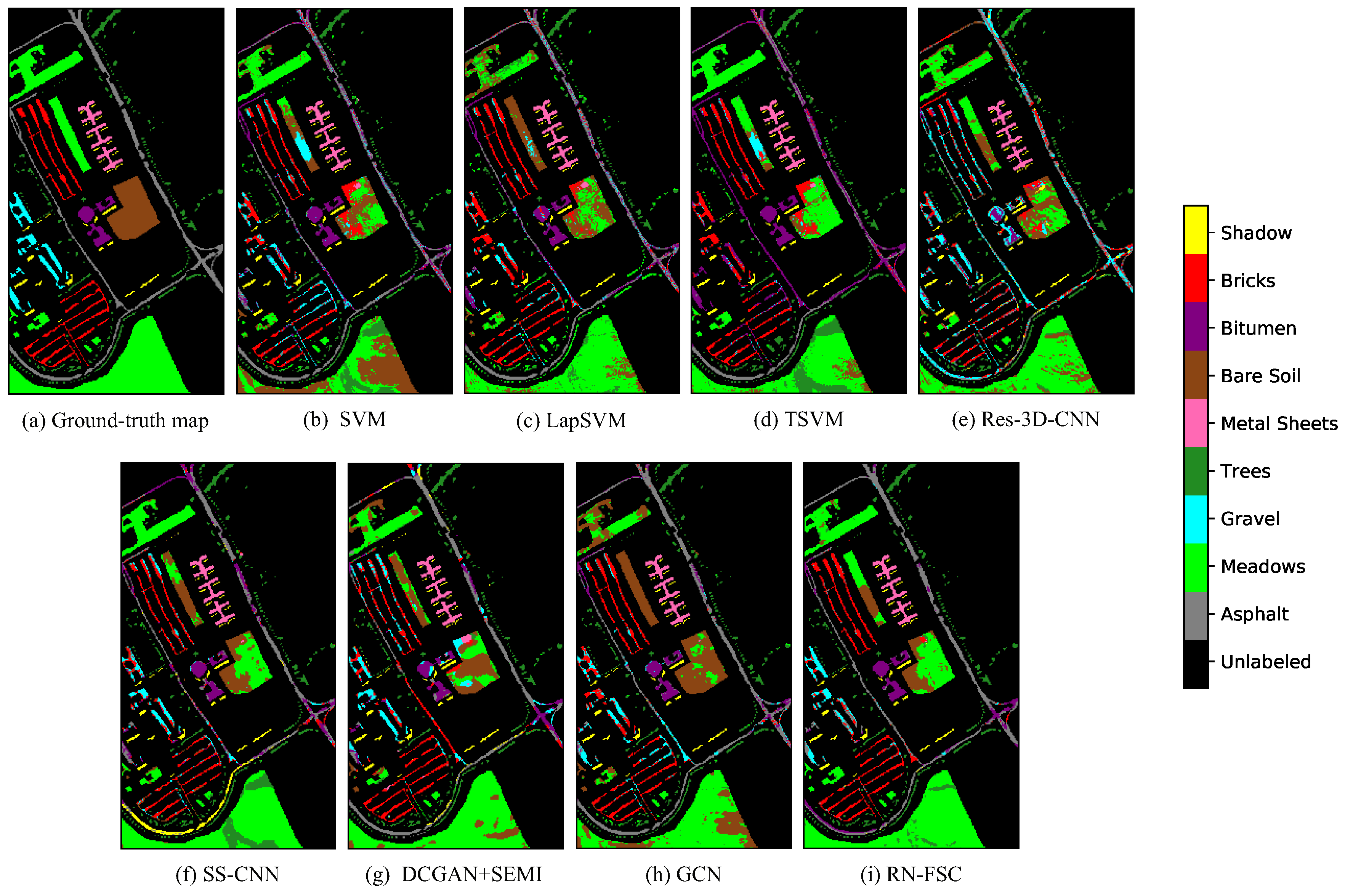
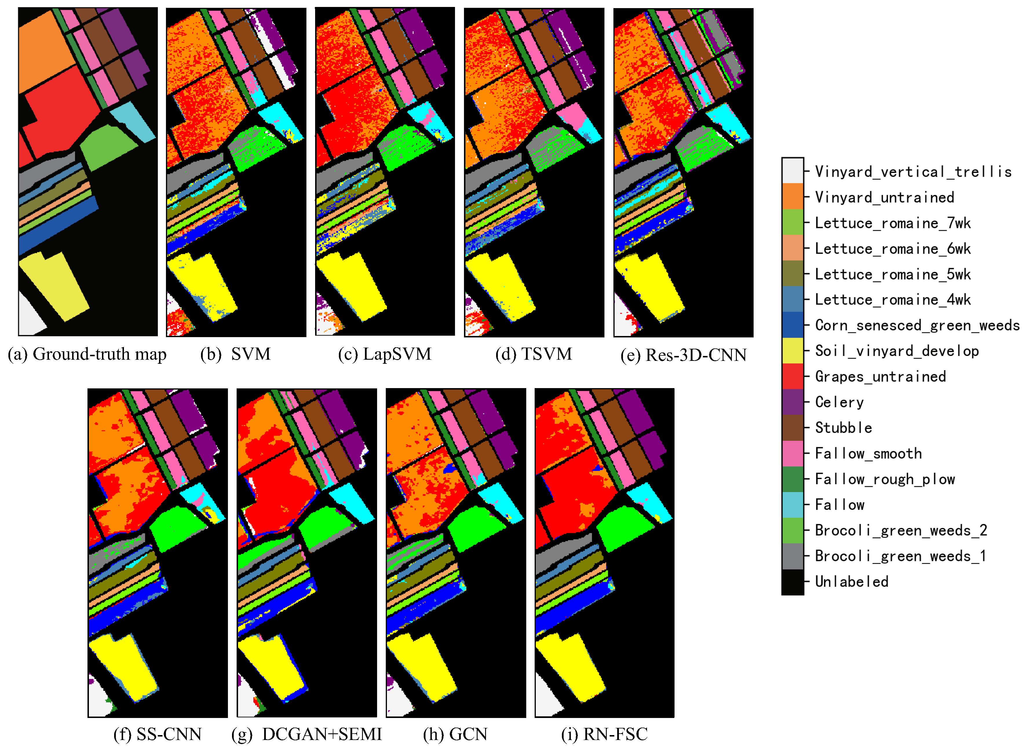
In order to verify the effectiveness of the proposed method in HSI few-shot classification, we compared the experimental results of RN-FSC with the widely used SVM, two classical semisupervised methods LapSVM and TSVM provided in [53], the deep learning model Res-3D-CNN [54], two semisupervised deep models SS-CNN [35] and DCGAN+SEMI [55], and the graph convolutional network (GCN) [56] model. SVM can map nonlinear data to linearly separable high-dimensional feature spaces utilizing the kernel method, so it can obtain a better classification effect than other traditional classifiers when processing high-dimensional HSI. LapSVM and TSVM are both classical semisupervised support vector machines. Res-3D-CNN constructs a deep classification model with the 3D convolutional layer and residual structure, which can make full use of the spatial–spectral information in HSI. By combining CNN and DCGAN with semisupervised learning, respectively, SS-CNN and DCGAN+SEMI can use the information of unlabeled samples for classification. GCN is also an advanced semisupervised classification model.
In order to quantitatively compare the classification performance of the above different methods, the overall accuracy (OA), classification accuracy per class, average accuracy (AA), and K a p p a coefficient are used as evaluation indicators. The overall accuracy is the percentage of samples classified correctly in all samples, and the average accuracy is the average of classification accuracy per class. It should be noted that for RN-FSC, five labeled samples per class in the target data set were used for fine-tuning, and for other methods, five labeled samples per class were used for training. Table 7, Table 8 and Table 9 summarize the experimental results on the three different target data sets, from which the following five observations can be obtained:
(1)
In general, the performance of the traditional SVM classifier is better than that of the supervised deep learning model. Deep learning models need sufficient training samples for parameter optimization. However, in the HSI few-shot classification problem, limited labeled samples cannot provide guarantee for enough training, so the performance of supervised deep learning models is worse than that of SVM. For example, the OA of SVM is 6.04% higher than that of Res-3D-CNN on the Salinas data set;
(2)
By comparing SVM and semisupervised SVM, Res-3D-CNN, and other semisupervised deep models, it can be found that the classification performance of the methods trained with only the labeled samples is poor. In this case, the semisupervised method can further improve the classification accuracy by utilizing the information of unlabeled samples;
(3)
The classification performance of the semisupervised deep model is always better than that of the traditional semisupervised SVM. Deep learning models can extract more discriminative features from labeled and unlabeled samples by building an end-to-end hierarchical framework, so they can obtain better classification results;
(4)
Compared with other methods, RN-FSC has the best classification performance, with the highest OA, AA, and K a p p a in all target data sets. The OA of RN-FSC is about 8.5%, 5%, and 6% higher than DCGAN+SEMI and GCN, which have similar performances on the three data sets. The most significant difference between RN-FSC and other methods is that other methods only perform training and classification on specific target data sets, while RN-FSC performs meta-learning on the collected source data sets through a large number of different tasks. Therefore, when processing new target data sets, RN-FSC has stronger generalization ability and can obtain better classification results with only a few labeled samples;
(5)
For the classes that other methods do not recognize accurately, RN-FSC can obtain better results, such as Bricks, Bare Soil and Gravel in UP, and Corn_senesced_green_weeds, Fallow in Salinas. Benefitting from meta-learning and network design, RN-FSC can acquire the ability to learn how to learn in the form of comparison. By comparing similarities between samples in the deep metric space, RN-FSC can take advantage of more abstract features. Therefore, RN-FSC can accurately recognize the uneasily distinguished classes.
In order to better compare and analyze the classification results of the above methods, Figure 12, Figure 13 and Figure 14 respectively show their classification maps on the three target data sets. With the continuous improvement of the classification accuracy, the noise and misclassification phenomena gradually decrease, and the classification map gradually approaches the ground-truth map. In fact, the results of Figure 12, Figure 13 and Figure 14 and Table 7, Table 8 and Table 9 are the same, both of which can prove the effectiveness of the proposed method.
In order to further verify that the observed increase in classification accuracy is statistically significant, we repeated the experiment 20 times for different methods and carried out the paired t-test on OA. The paired t-test is a widely used statistical method to verify whether there is a significant difference between the two groups of related samples [17,39]. In our test, if the result t is greater than 3.57, it indicates that there is a significant difference between the two groups of samples at the 99.9% confidence level. As seen from Table 10, all the results are greater than 3.57, indicating that the increase in classification accuracy is statistically significant.

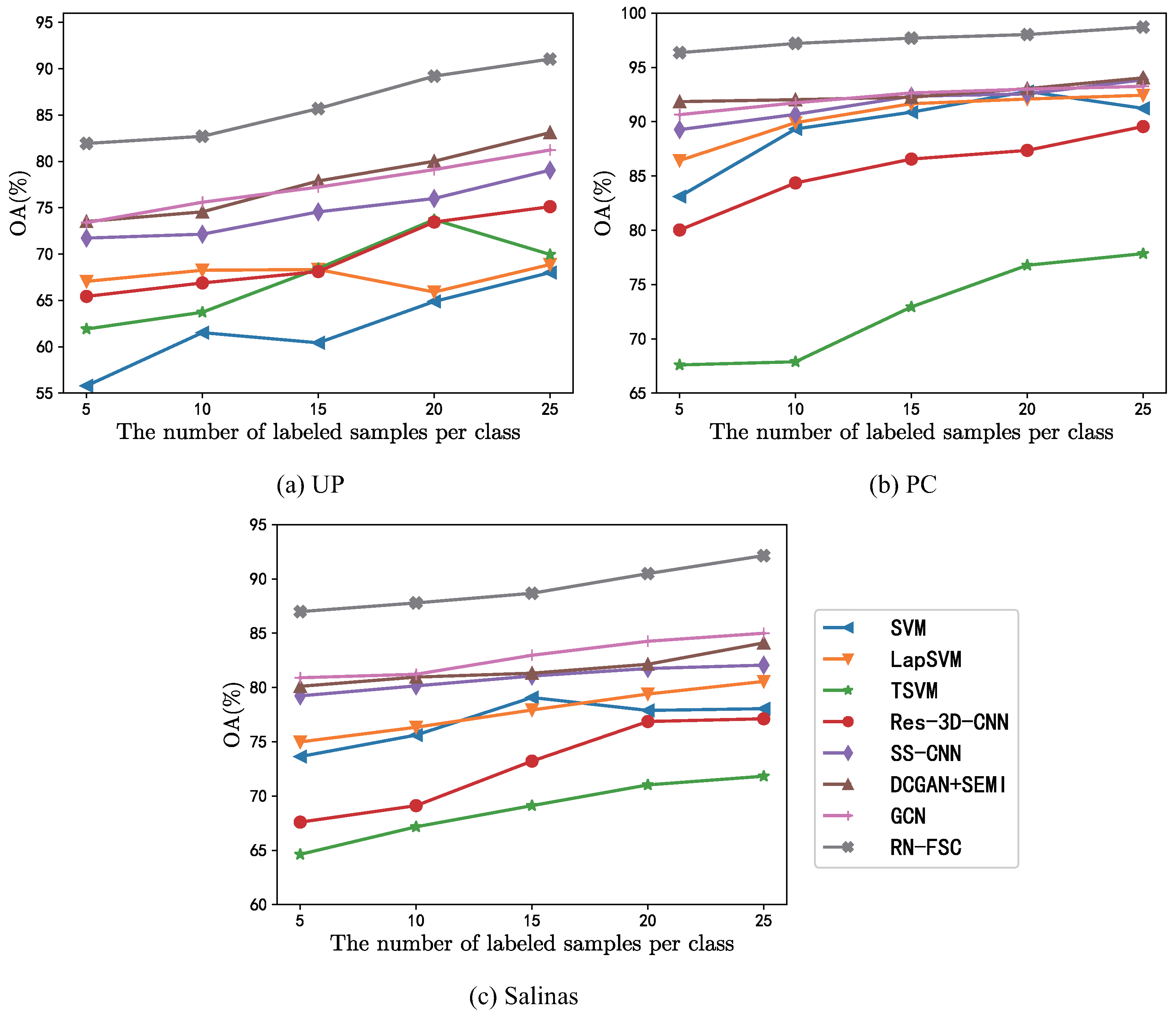
4.4. Influence of the Number of Labeled Samples

The objective of the experiments is to verify the classification effect of the proposed method on new HSI with only a few labeled samples. Therefore, it is necessary to explore the classification effect of the proposed method under different numbers of labeled samples. To this end, we randomly selected 5, 10, 15, 20, and 25 labeled samples per class to build the fine-tuning data set. Accordingly, we explored the classification results of other methods with 5, 10, 15, 20, and 25 labeled samples per class for training. Figure 15 shows the experimental results. It can be seen that the OA of all methods presents an increasing trend with the increase in the number of labeled samples. RN-FSC always has the highest classification accuracy, which indicates that it has the best adaptability to the number of labeled samples.
Experimental results from Table 7, Table 8 and Table 9 and Figure 15 have shown that the proposed method can achieve better classification results when classifying new HSI with only a few labeled samples. In order to further explore the influence of the number of labeled samples on the classification effect of RN-FSC, we conducted comparative experiments on Salinas and Indian Pines data sets with reference to [57,58,59]. The Indian Pines data set, containing 16 classes of the Indian Pine test site in Northwestern Indiana, was collected by AVIRIS. Salinas and Indian Pines both contain 16 classes, and Indian Pines contains 4 small classes with less than 100 labeled samples, which can further verify the effectiveness of the classification method. In the experiments, 10% and 2% labeled samples were randomly selected to build the fine-tuning data set (1083 labeled samples for Salinas and 1025 labeled samples for Indian Pines), which is far more than that of the previous experiments. It should be noted that the selection of labeled samples per class is exactly the same as in [57,58,59]. EPF-B-g, EPF-B-c, EPF-G-g, EPF-G-c, and IEPF-G-g provided in [57,58,59] were selected to make a comparison with the proposed method. Table 11 shows the experimental results. In the Salinas data set, the OA and AA of RN-FSC are higher than those of other methods. In the Indian Pines data set, the classification results of IEPF-G-g are the best, followed by those of RN-FSC. Overall, when the labeled samples are further increased (approximately 1000–1100 labeled samples for each data set), the proposed method can still obtain satisfactory results.

4.5. Exploration on the Effectiveness of Meta-Learning

The learning process of the proposed method, RN-FSC, can be divided into two phases: meta-learning on the source data set and few-shot learning on the fine-tuning data set. As mentioned in the previous sections, the reason RN-FSC has a better classification effect in the HSI few-shot classification is that it has acquired a large amount of feature knowledge and mastered the ability to learn how to learn through meta-learning. To verify this point, we carried out experiments to explore the influence of the meta-learning phase on the final classification results. Table 12 lists the overall accuracy with and without meta-learning with a different number of labeled samples. The model without meta-learning can only perform supervised training with a few labeled samples in the fine-tuning data set, so its classification results are poor. On the UP, PC, and Salinas data sets, the meta-learning phase can increase the classification accuracy by 20.20%, 10.73%, and 15.91%, respectively, when L = 5 , which fully proves the effectiveness of meta-learning in HSI few-shot classification. In addition, it can be found that with the increase in the number of labeled samples, the difference between the results with and without meta-learning shows a decreasing trend. For example, on the UP data set, the difference is 20.20% when L = 5 , and 10.83% when L = 25 .

4.6. Execution Time Analysis

The execution time of general deep learning models usually consists of training time and testing time. As described in Section 2.3, the proposed method consists of three phases: meta-learning, few-shot learning, and classification. The biggest difference between RN-FSC and other general deep models for HSI classification is that it first performs meta-learning on the previously collected source data sets and then classifies the new HSI data sets, which are absolutely different from the source data sets. In other words, only performing meta-learning in advance one time, RN-FSC can quickly classify all other new data sets, which is of great significance in practical applications. In our experiment, it takes approximately 12.83 h for the model to perform meta-learning. In practice, the model used to perform the classification task should have completed meta-learning. Therefore, the model needs only to perform few-shot learning and classification when processing the target HSI. Table 13 lists the execution times of DCGAN+SEMI, GCN, and RN-FSC on three different target data sets, because they present better classification results than other methods. DCGAN+SEMI and GCN include training and testing time, while RN-FSC includes few-shot learning time and classification time. DCGAN+SEMI needs to train the generator and the discriminator, respectively, while GCN utilizes all the labeled samples for graph construction, so their training time is longer. RN-FSC only utilizes a few labeled samples for fine-tuning, so the few-shot learning time is shorter. However, since RN-FSC needs to calculate the relation score through comparison, its classification time is longer. Generally speaking, the execution time of RN-FSC is shorter than that of DCGAN+SEMI and GCN, which indicates RN-FSC has better work efficiency.

4.7. Discussion

It is difficult for deep learning models to be fully trained and achieve promising classification results with a few labeled samples. At the same time, for complex and diverse HSI, the working mode that general deep learning models need to be trained from scratch every time is very inefficient and not desirable in practice. However, our method can obtain better classification results with only a few labeled samples (five samples per class) when processing new HSI. The root cause is the implementation of meta-learning, the core of which is the ability to learn how to learn. In our method, this ability is demonstrated in the form of comparison. Firstly, the model maps the data space to a deep metric space, where it performs relation learning by comparing the similarity of sample features, i.e., the similarity between samples belonging to the same class is high and the relation score is high, whereas the similarity between samples belonging to the different class is low and the relation score is low. In fact, the form of the ability to learn how to learn is not unique in the field of meta-learning, which largely depends on the specific network structure and loss function.
The task-based learning strategy is key to performing meta-learning. Lots of randomly generated tasks from different HSI can effectively enhance the generalization ability of the model, because the model learns how to compare with different tasks instead of how to classify a specific data set. To acquire the best learning effect, we explored the optimal task setting, including the number of classes, the number of support samples, and the number of query samples in the task. Experiments showed that the support samples should be much fewer than the query samples, so as to fully simulate the situation of HSI few-shot classification. In addition, experiments were conducted to explore the influence of learning rate to further optimize the meta-learning process. At the same time, the network structure can directly affect the classification results. A new deep model based on relation network was designed for HSI few-shot classification. In the feature learning module, the 3D convolutional layer can effectively utilize the spatial–spectral information to extract the highly discriminant features. In addition, we found that the convolutional layer is necessary in the relation learning module, which can guarantee the comparison ability of the model to some extent.
Through detailed comparison and analysis, it can be demonstrated that the proposed method outperforms SVM, semisupervised SVM, and several supervised and semisupervised deep learning models with a few labeled samples. Moreover, the proposed method has better adaptability to the number of samples. The paired t-test shows that the increase in classification accuracy is statistically significant and not accidental. In addition, by comparing the results of the model with and without meta-learning, the importance of the meta-learning phase is directly proved again. Finally, the efficiency of different methods was compared, indicating the potential value of the proposed method in practical application.

5. Conclusions

Although the deep learning model has achieved great success in HSI classification, it still faces great difficulties in classifying new HSI with a few labeled samples. To this end, this paper proposes a new classification method based on a relation network for HSI few-shot classification. Meta-learning is the core of this method, and the network settings realize the ability to learn how to learn in the form of comparison in deep metric space, that is, the relation score between samples belonging to the same class is high, while the relation score between samples belonging to different classes is low. Benefitting from a large number of tasks generated from different data sets, the generalization ability of the model is constantly enhanced. Experiments on three different target data sets show that the proposed method outperforms traditional semisupervised SVM and semisupervised deep learning methods when only a few labeled samples are available.

Author Contributions

Methodology, K.G. and B.L.; investigation, X.Y., J.Q., and P.Z.; resources, X.Y., P.Z., and X.T.; writing—original draft preparation, K.G.; writing—review and editing, K.G. and B.L.; visualization, J.Q. and X.T.; supervision, X.Y., P.Z., and X.T. All authors have read and agreed to the published version of the manuscript.

Funding

This research was funded by National Natural Science Foundation of China under Grant 41801388.

Acknowledgments

The authors would like to thank Yokoya for providing the data used in this study. The authors would also like to thank all the professionals for kindly providing the codes associated with the experiments.

Conflicts of Interest

The authors declare no conflict of interest.

References

  1. Sun, S.; Zhong, P.; Xiao, H.; Liu, F.; Wang, R. An active learning method based on SVM classifier for hyperspectral images classification. In Proceedings of the 7th Workshop on Hyperspectral Image and Signal Processing: Evolution in Remote Sensing (WHISPERS), Tokyo, Japan, 2–5 June 2015; pp. 1–4. [Google Scholar] [CrossRef]
  2. Yuemei, R.; Yanning, Z.; Wei, W.; Lei, L. A spectral-spatial hyperspectral data classification approach using random forest with label constraints. In Proceedings of the IEEE Workshop on Electronics, Computer and Applications, Ottawa, ON, Canada, 8–9 May 2014; pp. 344–347. [Google Scholar] [CrossRef]
  3. Agarwal, A.; El-Ghazawi, T.; El-Askary, H.; Le-Moigne, J. Efficient Hierarchical-PCA Dimension Reduction for Hyperspectral Imagery. In Proceedings of the IEEE International Symposium on Signal Processing and Information Technology, Cairo, Egypt, 15–18 December 2007; pp. 353–356. [Google Scholar] [CrossRef]
  4. Falco, N.; Bruzzone, L.; Benediktsson, J.A. An ICA based approach to hyperspectral image feature reduction. In Proceedings of the IEEE Geoscience and Remote Sensing Symposium, Quebec City, QC, Canada, 13–18 July 2014; pp. 3470–3473. [Google Scholar] [CrossRef]
  5. Li, C.; Chu, H.; Kuo, B.; Lin, C. Hyperspectral image classification using spectral and spatial information based linear discriminant analysis. In Proceedings of the IEEE International Geoscience and Remote Sensing Symposium, Vancouver, BC, Canada, 4–29 July 2011; pp. 1716–1719. [Google Scholar] [CrossRef]
  6. Liao, W.; Pizurica, A.; Philips, W.; Pi, Y. A fast iterative kernel PCA feature extraction for hyperspectral images. In Proceedings of the IEEE International Conference on Image Processing, Hong Kong, China, 26–29 September 2010; pp. 1317–1320. [Google Scholar] [CrossRef]
  7. Chen, Y.; Qu, C.; Lin, Z. Supervised Locally Linear Embedding based dimension reduction for hyperspectral image classification. In Proceedings of the IEEE International Geoscience and Remote Sensing Symposium—IGARSS, Melbourne, Australia, 21–26 July 2013; pp. 3578–3581. [Google Scholar] [CrossRef]
  8. Gao, L.; Gu, D.; Zhuang, L.; Ren, J.; Yang, D.; Zhang, B. Combining t-Distributed Stochastic Neighbor Embedding With Convolutional Neural Networks for Hyperspectral Image Classification. IEEE Geosci. Remote Sens. Lett. 2019, 1–5. [Google Scholar] [CrossRef]
  9. Quesada-Barriuso, P.; Argüello, F.; Heras, D.B. Spectral–Spatial Classification of Hyperspectral Images Using Wavelets and Extended Morphological Profiles. IEEE J. Sel. Topics Appl. Earth Obs. Remote Sens. 2014, 7, 1177–1185. [Google Scholar] [CrossRef]
  10. Jia, S.; Hu, J.; Zhu, J.; Jia, X.; Li, Q. Three-Dimensional Local Binary Patterns for Hyperspectral Imagery Classification. IEEE Trans. Geosci. Remote Sens. 2017, 55, 2399–2413. [Google Scholar] [CrossRef]
  11. Bau, T.C.; Sarkar, S.; Healey, G. Hyperspectral Region Classification Using a Three-Dimensional Gabor Filterbank. IEEE Trans. Geosci. Remote Sens. 2010, 48, 3457–3464. [Google Scholar] [CrossRef]
  12. Xu, Y.; Wu, Z.; Wei, Z. Markov random field with homogeneous areas priors for hyperspectral image classification. In Proceedings of the IEEE Geoscience and Remote Sensing Symposium, Quebec City, QC, Canada, 13–18 July 2014; pp. 3426–3429. [Google Scholar] [CrossRef]
  13. He, L.; Chen, X. A three-dimensional filtering method for spectral-spatial hyperspectral image classification. In Proceedings of the IEEE International Geoscience and Remote Sensing Symposium (IGARSS), Beijing, China, 10–15 July 2016; pp. 2746–2748. [Google Scholar] [CrossRef]
  14. Casalino, G.; Gillis, N. Sequential dimensionality reduction for extracting localized features. Pattern Recognit. 2017, 63, 15–29. [Google Scholar] [CrossRef] [Green Version]
  15. Yin, J.; Li, S.; Zhu, H.; Luo, X. Hyperspectral Image Classification Using CapsNet With Well-Initialized Shallow Layers. IEEE Geosci. Remote Sens. Lett. 2019, 16, 1095–1099. [Google Scholar] [CrossRef]
  16. Zhang, L.; Zhang, L.; Du, B. Deep Learning for Remote Sensing Data: A Technical Tutorial on the State of the Art. IEEE Geosci. Remote Sens. Mag. 2016, 4, 22–40. [Google Scholar] [CrossRef]
  17. Chen, Y.; Lin, Z.; Zhao, X.; Wang, G.; Gu, Y. Deep Learning-Based Classification of Hyperspectral Data. IEEE J. Sel.Topics Appl. Earth Obs. Remote Sens. 2014, 7, 2094–2107. [Google Scholar] [CrossRef]
  18. Mou, L.; Ghamisi, P.; Zhu, X.X. Deep Recurrent Neural Networks for Hyperspectral Image Classification. IEEE Trans. Geosci. Remote Sens. 2017, 55, 3639–3655. [Google Scholar] [CrossRef] [Green Version]
  19. Hang, R.; Liu, Q.; Hong, D.; Ghamisi, P. Cascaded Recurrent Neural Networks for Hyperspectral Image Classification. IEEE Trans. Geosci. Remote Sens. 2019, 57, 5384–5394. [Google Scholar] [CrossRef] [Green Version]
  20. Chen, Y.; Zhao, X.; Jia, X. Spectral–Spatial Classification of Hyperspectral Data Based on Deep Belief Network. IEEE J. Sel. Topics Appl. Earth Obs. Remote Sens. 2015, 8, 2381–2392. [Google Scholar] [CrossRef]
  21. Mughees, A.; Tao, L. Multiple deep-belief-network-based spectral-spatial classification of hyperspectral images. Tsinghua Sci. Technol. 2019, 24, 183–194. [Google Scholar] [CrossRef]
  22. He, L.; Li, J.; Liu, C.; Li, S. Recent Advances on Spectral–Spatial Hyperspectral Image Classification: An Overview and New Guidelines. IEEE Trans. Geosci. Remote Sens. 2018, 56, 1579–1597. [Google Scholar] [CrossRef]
  23. Zhang, M.; Li, W.; Du, Q. Diverse Region-Based CNN for Hyperspectral Image Classification. IEEE Trans. Image Process. 2018, 27, 2623–2634. [Google Scholar] [CrossRef]
  24. Lee, H.; Kwon, H. Going Deeper With Contextual CNN for Hyperspectral Image Classification. IEEE Trans. Image Process. 2017, 26, 4843–4855. [Google Scholar] [CrossRef] [Green Version]
  25. Zhi, L.; Yu, X.; Liu, B.; Wei, X. A dense convolutional neural network for hyperspectral image classification. Remote Sens. Lett. 2019, 10, 59–66. [Google Scholar] [CrossRef]
  26. Zhang, H.; Li, Y.; Zhang, Y.; Shen, Q. Spectral-spatial classification of hyperspectral imagery using a dual-channel convolutional neural network. Remote Sens. Lett. 2017, 8, 438–447. [Google Scholar] [CrossRef] [Green Version]
  27. Chen, Y.; Jiang, H.; Li, C.; Jia, X.; Ghamisi, P. Deep Feature Extraction and Classification of Hyperspectral Images Based on Convolutional Neural Networks. IEEE Trans. Geosci. Remote Sens. 2016, 54, 6232–6251. [Google Scholar] [CrossRef] [Green Version]
  28. Zhong, Z.; Li, J.; Luo, Z.; Chapman, M. Spectral–Spatial Residual Network for Hyperspectral Image Classification: A 3-D Deep Learning Framework. IEEE Trans. Geosci. Remote Sens. 2018, 56, 847–858. [Google Scholar] [CrossRef]
  29. Fang, B.; Li, Y.; Zhang, H.; Chan, J. Hyperspectral Images Classification Based on Dense Convolutional Networks with Spectral-Wise Attention Mechanism. Remote Sens. 2019, 11, 159. [Google Scholar] [CrossRef] [Green Version]
  30. Li, A.; Shang, Z. A new Spectral-Spatial Pseudo-3D Dense Network for Hyperspectral Image Classification. In Proceedings of the International Joint Conference on Neural Networks (IJCNN), Budapest, Hungary, 14–19 July 2019; pp. 1–7. [Google Scholar] [CrossRef]
  31. Xu, Q.; Xiao, Y.; Wang, D.; Luo, B. CSA-MSO3DCNN: Multiscale Octave 3D CNN with Channel and Spatial Attention for Hyperspectral Image Classification. Remote Sens. 2020, 12, 188. [Google Scholar] [CrossRef] [Green Version]
  32. Jamshidpour, N.; Aria, E.H.; Safari, A.; Homayouni, S. Adaptive Self-Learned Active Learning Framework for Hyperspectral Classification. In Proceedings of the 10th Workshop on Hyperspectral Imaging and Signal Processing: Evolution in Remote Sensing (WHISPERS), Amsterdam, The Netherlands, 24–26 September 2019; pp. 1–5. [Google Scholar] [CrossRef]
  33. Paoletti, M.E.; Haut, J.M.; Fernandez-Beltran, R.; Plaza, J.; Plaza, A.; Li, J.; Pla, F. Capsule Networks for Hyperspectral Image Classification. IEEE Trans. Geosci. Remote Sens. 2019, 57, 2145–2160. [Google Scholar] [CrossRef]
  34. Fan, J.; Tan, H.L.; Toomik, M.; Lu, S. Spectral-spatial hyperspectral image classification using super-pixel-based spatial pyramid representation. In Image and Signal Processing for Remote Sensing XXII; Bruzzone, L., Bovolo, F., Eds.; International Society for Optics and Photonics, SPIE: San Francisco, CA, USA, 2016; Volume 10004, pp. 315–321. [Google Scholar] [CrossRef]
  35. Liu, B.; Yu, X.; Zhang, P.; Tan, X.; Yu, A.; Xue, Z. A semi-supervised convolutional neural network for hyperspectral image classification. Remote Sens. Lett. 2017, 8, 839–848. [Google Scholar] [CrossRef]
  36. Wu, Y.; Mu, G.; Qin, C.; Miao, Q.; Ma, W.; Zhang, X. Semi-Supervised Hyperspectral Image Classification via Spatial-Regulated Self-Training. Remote Sens. 2020, 12, 159. [Google Scholar] [CrossRef] [Green Version]
  37. Kang, X.; Zhuo, B.; Duan, P. Semi-supervised deep learning for hyperspectral image classification. Remote Sens. Lett. 2019, 10, 353–362. [Google Scholar] [CrossRef]
  38. Li, W.; Wu, G.; Zhang, F.; Du, Q. Hyperspectral Image Classification Using Deep Pixel-Pair Features. IEEE Trans. Geosci. Remote Sens. 2017, 55, 844–853. [Google Scholar] [CrossRef]
  39. Liu, B.; Yu, X.; Zhang, P.; Yu, A.; Fu, Q.; Wei, X. Supervised Deep Feature Extraction for Hyperspectral Image Classification. IEEE Trans. Geosci. Remote Sens. 2018, 56, 1909–1921. [Google Scholar] [CrossRef]
  40. Xu, S.; Mu, X.; Chai, D.; Zhang, X. Remote sensing image scene classification based on generative adversarial networks. Remote Sens. Lett. 2018, 9, 617–626. [Google Scholar] [CrossRef]
  41. Qin, J.; Zhan, Y.; Wu, K.; Liu, W.; Yang, Z.; Yao, W.; Medjadba, Y.; Zhang, Y.; Yu, X. Semi-Supervised Classification of Hyperspectral Data for Geologic Body Based on Generative Adversarial Networks at Tianshan Area. In Proceedings of the IGARSS 2018—2018 IEEE International Geoscience and Remote Sensing Symposium, Valencia, Spain, 22–27 July 2018; pp. 4776–4779. [Google Scholar] [CrossRef]
  42. Wang, H.; Tao, C.; Qi, J.; Li, H.; Tang, Y. Semi-Supervised Variational Generative Adversarial Networks for Hyperspectral Image Classification. In Proceedings of the IGARSS 2019—2019 IEEE International Geoscience and Remote Sensing Symposium, Yokohama, Japan, 28 July–2 August 2019; pp. 9792–9794. [Google Scholar] [CrossRef]
  43. Ren, M.; Triantafillou, E.; Ravi, S.; Snell, J.; Swersky, K.; Tenenbaum, J.; Larochelle, H.; Zemel, R. Meta-Learning for Semi-Supervised Few-Shot Classification. arXiv 2018, arXiv:1803.00676. [Google Scholar]
  44. Finn, C.; Abbeel, P.; Levine, S. Model-Agnostic Meta-Learning for Fast Adaptation of Deep Networks. arXiv 2017, arXiv:1703.03400. [Google Scholar]
  45. Andrychowicz, M.; Denil, M.; Gómez, S.; Hoffman, M.; Pfau, D.; Schaul, T.; Freitas, N. Learning to learn by gradient descent by gradient descent. arXiv 2016, arXiv:1606.04474. [Google Scholar]
  46. Li, Z.; Zhou, F.; Chen, F.; Li, H. Meta-SGD: Learning to Learn Quickly for Few Shot Learning. arXiv 2017, arXiv:1707.09835. [Google Scholar]
  47. Liang, H.; Fu, W.; Yi, F. A Survey of Recent Advances in Transfer Learning. In Proceedings of the IEEE 19th International Conference on Communication Technology (ICCT), Xi’an, China, 16–19 October 2019; pp. 1516–1523. [Google Scholar] [CrossRef]
  48. Liu, B.; Yu, X.; Yu, A.; Wan, G. Deep convolutional recurrent neural network with transfer learning for hyperspectral image classification. J. Appl. Remote Sens. 2018, 12, 1. [Google Scholar] [CrossRef]
  49. Sung, F.; Yang, Y.; Zhang, L.; Xiang, T.; Torr, P.; Hospedales, T. Learning to Compare: Relation Network for Few-Shot Learning. In Proceedings of the IEEE/CVF Conference on Computer Vision and Pattern Recognition, Salt Lake City, UT, USA, 18–23 June 2018; pp. 1199–1208. [Google Scholar] [CrossRef] [Green Version]
  50. Lin, M.; Chen, Q.; Yan, S. Network In Network. arXiv 2013, arXiv:1312.4400. [Google Scholar]
  51. Sun, V.; Geng, X.; Chen, J.; Ji, L.; Tang, H.; Zhao, Y.; Xu, M. A robust and efficient band selection method using graph representation for hyperspectral imagery. Int. J. Remote Sens. 2016, 37, 4874–4889. [Google Scholar] [CrossRef]
  52. Glorot, X.; Bengio, Y. Understanding the difficulty of training deep feedforward neural networks. J. Mach. Learn. Res. Proc. Track 2010, 9, 249–256. [Google Scholar]
  53. Wang, L.; Hao, S.; Wang, Q.; Wang, Y. Semi-supervised classification for hyperspectral imagery based on spatial-spectral Label Propagation. ISPRS J. Photogramm. Remote Sens. 2014, 97, 123–137. [Google Scholar] [CrossRef]
  54. Liu, B.; Yu, X.; Zhang, P.; Tan, X. Deep 3D convolutional network combined with spatial-spectral features for hyperspectral image classification. Cehui Xuebao/Acta Geodaetica et Cartographica Sinica 2019, 48, 53–63. [Google Scholar] [CrossRef]
  55. Salimans, T.; Goodfellow, I.; Zaremba, W.; Cheung, V.; Radford, A.; Chen, X. Improved Techniques for Training GANs. arXiv 2016, arXiv:1606.03498. [Google Scholar]
  56. Kipf, T.; Welling, M. Semi-Supervised Classification with Graph Convolutional Networks. arXiv 2016, arXiv:1609.02907. [Google Scholar]
  57. Kang, X.; Li, S.; Benediktsson, J.A. Spectral-Spatial Hyperspectral Image Classification With Edge-Preserving Filtering. IEEE Transm Geoscim Remote Sens. 2014, 52, 2666–2677. [Google Scholar] [CrossRef]
  58. Zhong, S.; Chang, C.I.; Zhang, Y. Iterative Edge Preserving Filtering Approach to Hyperspectral Image Classification. IEEE Geosci. Remote Sens. Lett. 2018. [Google Scholar] [CrossRef]
  59. Zhong, S.; Chang, C.; Li, J.; Shang, X.; Chen, S.; Song, M.; Zhang, Y. Class Feature Weighted Hyperspectral Image Classification. IEEE J. Sel. Topics Appl. Earth Obs. Remote Sens. 2019, 12, 4728–4745. [Google Scholar] [CrossRef]
Figure 1. Definition of few-shot classification.
Remotesensing 12 00923 g001
Figure 2. Different training and learning strategy where color represents class. (a) Batch-based training strategy used widely in deep learning. (b) Task-based learning strategy used in meta-learning.
Remotesensing 12 00923 g002
Figure 3. Visual representation of the designed relation network model for HSI few-shot classification.
Remotesensing 12 00923 g003
Figure 4. Visual representation of the feature learning module.
Remotesensing 12 00923 g004
Figure 5. Visual representation of the relation learning module.
Remotesensing 12 00923 g005
Figure 6. Houston data set. (a) Pseudocolor image. (b) Ground-truth map.
Remotesensing 12 00923 g006
Figure 7. Botswana data set. (a) Pseudocolor image. (b) Ground-truth map.
Remotesensing 12 00923 g007
Figure 8. Kennedy Space Center (KSC) data set. (a) Pseudocolor image. (b) Ground-truth map.
Remotesensing 12 00923 g008
Figure 9. Chikusei data set. (a) Pseudocolor image. (b) Ground-truth map.
Remotesensing 12 00923 g009
Figure 10. Overall accuracy under different C.
Remotesensing 12 00923 g010
Figure 11. Loss value under different learning rates.
Remotesensing 12 00923 g011
Figure 12. Classification maps resulting from different methods on the UP data set.
Remotesensing 12 00923 g012
Figure 13. Classification maps resulting from different methods on the PC data set.
Remotesensing 12 00923 g013
Figure 14. Classification maps resulting from different methods on the SA data set.
Remotesensing 12 00923 g014
Figure 15. Classification accuracy under different number of labeled samples on three target data sets.
Remotesensing 12 00923 g015
Table 1. Detailsof the source data sets. Kennedy Space Center (KSC), ground sample distance (GSD)(m), spatial size (pixel), spectral range (nm), airborne visible infrared imaging spectrometer (AVIRIS).
HoustonBotswanaKSCChikusei
Spatial size 349 × 1905 1476 × 256 512 × 614 2517 × 2335
Spectral range380–1050400–2500400–2500363–1018
No. of bands144145176128
GSD2.530182.5
Sensor typeITRES-CASI 1500EO-1AVIRISHyperspec-VNIR-C
AreasHoustonBotswanaFloridaChikusei
No. of classes30141319
Labeled samples15,0293248521177,592
Table 2. The selected bands on the source data sets via graph-representation-based band selection (GRBS). Kennedy Space Center (KSC).
The Selected Bands
Houston2 3 4 5 6 7 8 9 10 11 12 13 14 15 16 17 18 19 20 21 22 23 24 25 26 27 28 29 30 31 32 33 34 35 36 37 38 39 40 41 42 43 44 45 46 47 48 49 51 52 53 54 55 56 57 58 59 60 61 62 63 64 65 66 67 68 69 70 71 72 77 107 109 110 111 112 113 114 115 116 117 118 119 120 121 122 123 124 125 126 127 128 129 130 132 133 134 135 143 144
Botswana2 3 4 5 6 7 8 9 10 11 12 13 14 15 16 17 18 19 20 21 22 23 24 25 26 27 28 29 30 31 32 33 34 35 36 37 38 39 40 41 42 43 44 45 46 47 48 49 50 51 52 53 55 56 57 58 59 60 61 62 63 64 65 66 67 68 69 70 71 72 73 88 110 111 112 113 114 115 116 117 118 119 120 121 122 123 124 125 126 127 128 137 138 139 140 141 142 143 144 145
KSC2 3 4 5 6 7 8 9 10 11 12 13 14 15 16 17 18 19 20 21 22 23 24 25 26 28 29 31 32 33 35 36 37 39 40 41 42 43 44 45 46 47 48 49 50 51 52 53 54 55 56 57 58 59 60 61 62 63 64 65 66 67 68 71 72 73 74 75 76 77 78 79 80 81 82 83 84 85 86 87 88 89 90 95 101 120 132 143 144 145 146 147 148 149 150 151 155 167 175 176
Chikusei1 2 3 4 5 6 7 8 9 10 11 12 13 14 15 16 17 18 19 20 21 22 23 24 25 26 27 28 29 30 31 32 33 34 35 36 37 38 39 40 41 42 43 44 45 46 47 48 49 50 51 52 53 54 55 56 57 58 59 60 61 62 63 65 66 67 94 95 96 97 98 99 100 101 102 103 104 105 106 107 108 109 110 111 112 113 114 116 117 118 119 120 121 122 123 124 125 126 127 128
Table 3. Details of three target data sets. University of Pavia (UP), Pavia Center (PC), ground sample distance (GSD) (m), spatial size (pixel), spectral range (nm), reflective optics system imaging spectrometer (ROSIS), airborne visible infrared imaging spectrometer (AVIRIS).
UPPCSalinas
Spatial size 610 × 340 1096 × 715 512 × 217
Spectral range430–860430–860400–2500
No. of bands103102204
GSD1.31.33.7
Sensor typeROSISROSISAVIRIS
AreasPaviaPaviaCalifornia
No. of classes9916
Labeled samples42,776148,15254,129
Table 4. The selected bands on the target data sets via GRBS. University of Pavia (UP), Pavia Center (PC).
The Selected Bands
UP2 3 4 5 6 7 8 9 10 11 12 13 14 15 16 17 18 19 20 21 23 24 25 26 27 28 29 30 31 32 33 34 35 36 37 38 39 40 41 42 43 44 45 46 47 48 49 50 51 53 54 55 56 57 58 59 60 61 62 63 64 65 66 67 68 69 70 71 72 73 74 75 76 77 78 79 80 81 82 83 84 85 86 87 88 89 90 91 92 93 94 95 96 97 98 99 100 101 102 103
PC1 2 3 4 5 6 7 8 9 10 11 12 13 14 15 16 17 18 19 21 22 23 24 25 26 27 28 29 30 31 32 33 34 35 36 37 38 39 40 41 42 43 44 45 46 47 48 49 50 51 52 53 54 55 56 57 58 60 61 62 63 64 65 66 67 68 69 70 71 72 73 74 75 76 77 78 79 80 81 82 83 84 85 86 87 88 89 90 91 92 93 94 95 96 97 98 99 100 101 102
Salinas2 3 4 5 6 7 8 9 10 11 12 13 14 15 16 17 18 19 20 21 22 23 24 25 26 27 28 29 31 33 34 35 36 37 38 39 40 41 42 43 44 45 46 47 48 49 50 51 52 53 54 55 56 57 58 59 60 61 62 63 64 65 66 67 68 69 70 71 72 73 74 75 76 77 78 79 80 81 82 83 84 85 86 87 88 89 90 91 92 93 94 95 96 97 98 99 100 126 139 204
Table 5. Overall accuracy (%) with different combinations of K and N.
K = 1, N = 19K = 5, N = 15K = 10, N = 10K = 15, N = 5
UP 81.94 78.84 76.26 74.55
PC 96.36 96.03 95.53 94.89
Salinas 86.99 85.97 84.61 82.95
Table 6. Overall classification accuracy (OA, %) on the UP data set under different network structure settings. The feature learning module (FLM), the relation learning module (RLM), max pooling (MP), fully connected layer (FC).
No.1234567
FLM 3 × 3 × 3 ( 8 ) 3 × 3 × 3 ( 16 ) 2 × 2 × 4 MP 3 × 3 × 3 ( 32 ) 3 × 3 × 3 ( 64 ) 2 × 2 × 4 MP 3 × 3 × 3 ( 8 ) 2 × 2 × 4 MP 3 × 3 × 3 ( 16 ) 2 × 2 × 4 MP 3 × 3 × 3 ( 32 ) 3 × 3 × 3 ( 8 ) 2 × 2 × 4 MP 3 × 3 × 3 ( 16 ) 2 × 2 × 4 MP 3 × 3 × 3 ( 8 ) 4 × 4 × 8 MP 3 × 3 × 3 ( 8 ) 2 × 2 × 4 MP 3 × 3 × 3 ( 16 ) 2 × 2 × 4 MP 3 × 3 × 3 ( 32 ) 3 × 3 × 3 ( 8 ) 2 × 2 × 4 MP 3 × 3 × 3 ( 16 ) 2 × 2 × 4 MP 3 × 3 × 3 ( 32 ) 3 × 3 × 3 ( 8 ) 2 × 2 × 4 MP 3 × 3 × 3 ( 16 ) 2 × 2 × 4 MP 3 × 3 × 3 ( 32 )
RLM 1 × 1 ( 64 ) 3 × 3 ( 128 ) 2 × 2 MP 128 FC 1 FC 1 × 1 ( 64 ) 3 × 3 ( 128 ) 2 × 2 MP 128 FC 1 FC 1 × 1 ( 64 ) 3 × 3 ( 128 ) 2 × 2 MP 128 FC 1 FC 1 × 1 ( 64 ) 3 × 3 ( 128 ) 2 × 2 MP 128 FC 1 FC 1 × 1 ( 64 ) 3 × 3 ( 128 ) 3 × 3 ( 256 ) 2 × 2 MP 128 FC 1 FC 3 × 3 ( 128 ) 2 × 2 MP 128 F C 1 FC 1024 FC 512 FC 1 FC
OA80.3781.9479.5075.4377.8378.3726.55
Table 7. Classification results of the different methods on the UP data set (5 samples per class in the fine-tuning data set for RN-FSC; 5 samples per class are used for training for other methods; bold values represent the best results among these methods).
ClassSVMLapSVMTSVMRes-3D-CNNSS-CNNDCGAN+SEMIGCNRN-FSC
Asphalt94.0898.1296.5571.6789.8992.1896.0087.28
Meadows79.0381.5780.4788.9684.4090.3293.3984.33
Gravel27.6730.9711.1123.3059.9441.8050.7190.42
Trees57.7162.4748.7188.8657.9486.3995.8578.09
Metal Sheets91.6791.3994.9289.3997.1183.3099.1999.56
Bare Soil21.1037.7837.9137.8853.0143.6337.5463.25
Bitumen35.3337.6720.5038.6236.1544.5457.2652.09
Bricks57.3160.4755.3642.5972.7062.1173.3184.81
Shadow99.7999.8999.8963.1348.6566.3398.1395.94
OA55.7967.0661.9265.4471.7373.5273.4081.94
AA62.6366.7060.6060.4966.6467.8477.9381.75
K a p p a 46.6057.9051.4455.6363.3766.0766.9675.84
Table 8. Classification results of the different methods on the PC data set (5 samples per class in the fine-tuning data set for RN-FSC; 5 samples per class are used for training for other methods; bold values represent the best results among these methods).
ClassSVMLapSVMTSVMRes-3D-CNNSS-CNNDCGAN+SEMIGCNRN-FSC
Water99.9599.9995.1299.9999.1798.1399.74100.00
Trees94.6894.7592.2274.1793.3498.1599.3699.53
Meadows40.8660.8440.1280.2475.1765.8161.5367.60
Bricks56.4714.578.1227.1168.8555.6468.2272.43
Bare Soil19.5165.4727.1523.0838.2553.4242.7796.91
Asphalt63.6661.8546.8767.6981.4284.2181.6285.86
Bitumen78.2192.831.3877.3875.8299.3791.6185.55
Tile88.6694.5597.1498.8899.5799.0299.0699.94
Shadow99.7699.8693.1787.6195.6077.4698.0091.87
OA83.1186.4367.6080.0389.2791.8590.6596.36
AA71.3176.0855.7070.6980.8081.2482.4388.86
K a p p a 76.6281.2256.6073.1688.3091.0289.7995.98
Table 9. Classification results of the different methods on the Salinas data set (5 samples per class in the fine-tuning data set for RN-FSC; 5 samples per class are used for training for other methods; bold values represent the best results among these methods).
ClassSVMLapSVMTSVMRes-3D-CNNSS-CNNDCGAN+SEMIGCNRN-FSC
Brocoli_green_weeds_185.6078.5980.5039.4793.0256.94100.0099.26
Brocoli_green_weeds_298.5498.9998.0874.0292.5171.5381.95100.00
Fallow65.3882.9665.1949.3384.3187.4483.5097.87
Fallow_rough_plow95.8296.6495.4688.7186.4376.4596.9999.50
Fallow_smooth95.8388.0964.2577.5090.9194.9596.9697.81
Stubble99.92100.0099.9597.5299.5599.4799.8299.35
Celery95.2989.6185.1061.5397.5489.6394.66100.00
Grapes_untrained57.0063.8744.2968.9373.5270.9386.0066.24
Soil_vinyard_develop90.6479.4974.0692.8393.8192.8995.6597.34
Corn_senesced_green_weeds85.8756.5564.7169.3377.2163.5881.3193.66
Lettuce_romaine_4wk38.3238.0247.5659.0742.3783.8160.0573.96
Lettuce_romaine_5wk87.5692.7192.5670.5995.8597.3395.6599.84
Lettuce_romaine_6wk88.6646.8847.8775.3899.2397.5389.39100.00
Lettuce_romaine_7wk87.8793.2686.8189.1292.9887.0986.4196.39
Vinyard_untrained33.1849.8432.3147.6250.3774.7851.0068.85
Vinyard_vertical_trellis81.6491.0054.2488.9080.5477.1795.0799.89
OA73.6474.9964.6367.6079.2380.1180.9086.99
AA80.4577.9170.8171.8784.3882.6097.1593.12
K a p p a 70.7072.0560.9564.2877.0477.8678.9585.44
Table 10. Results of the paired t-test on three target data sets.
University of PaviaPavia CenterSalinas
t/significant?t/significant?t/significant?
RN-FSC vs. SVM
75.53/yes26.34/yes34.40/yes
RN-FSC vs. LapSVM
24.36/yes34.79/yes33.75/yes
RN-FSC vs. TSVM
47.44/yes71.68/yes37.29/yes
RN-FSC vs. Res-3D-CNN
35.62/yes30.08/yes29.19/yes
RN-FSC vs. SS-CNN
27.17/yes22.60/yes19.33/yes
RN-FSC vs. DCGAN+SEMI
23.56/yes19.88/yes16.86/yes
RN-FSC vs. GCN
21.05/yes20.05/yes15.98/yes
Table 11. Classification results of the different methods on Salinas and Indian Pines.
The Target Data Set EPF-B-gEPF-B-cEPF-G-gEPF-G-cIEPF-G-gRN-FSC
SalinasOA
AA
96.46
98.17
96.23
98.08
96.61
98.24
97.11
98.56
98.36
99.19
98.86
99.26
Indian PinesOA
AA
94.82
95.96
95.30
95.44
93.94
96.64
94.87
96.52
98.19
98.67
97.46
96.68
Table 12. Influence of the meta-learning phase on classification accuracy (OA, %). L is the number of labeled samples per class.
Target
Data Set
Meta-Learning L = 5 L = 10 L = 15 L = 20 L = 25
UPyes81.9482.7185.7089.2091.05
not61.7469.5674.1278.9380.22
PCyes96.3697.2197.7098.0398.72
not85.6386.4687.4190.5392.10
Salinasyes86.9987.7988.6890.4992.15
not71.0874.0875.9677.3480.45
Table 13. Execution times on three target data sets (5 samples per class are used as labeled samples).
Target
Data Set
DCGAN+SEMIGCNRN-FSC
UP1355.86 ( s ) + 2.57 ( s ) 1915.29 ( s ) + 0.98 ( s ) 217.27 ( s ) + 72.57 ( s )
PC1401.31 ( s ) + 8.13 ( s ) 3042.18 ( s ) + 1.44 ( s ) 214.98 ( s ) + 198.09 ( s )
Salinas2386.74 ( s ) + 3.03 ( s ) 1224.03 ( s ) + 1.10 ( s ) 632.98 ( s ) + 81.23 ( s )

