GF-5 Hyperspectral Data for Species Mapping of Mangrove in Mai Po, Hong Kong

Abstract

Hyperspectral data has been widely used in species discrimination of plants with rich spectral information in hundreds of spectral bands, while the availability of hyperspectral data has hindered its applications in many specific cases. The successful operation of the Chinese satellite, Gaofen-5 (GF-5), provides potentially promising new hyperspectral dataset with 330 spectral bands in visible and near infrared range. Therefore, there is much demand for assessing the effectiveness and superiority of GF-5 hyperspectral data in plants species mapping, particularly mangrove species mapping, to better support the efficient mangrove management. In this study, mangrove forest in Mai Po Nature Reserve (MPNR), Hong Kong was selected as the study area. Four dominant native mangrove species were investigated in this study according to the field surveys. Two machine learning methods, Random Forests and Support Vector Machines, were employed to classify mangrove species with Landsat 8, Simulated Hyperion and GF-5 data sets. The results showed that 97 more bands of GF-5 over Hyperion brought a higher over accuracy of 87.12%, in comparison with 86.82% from Hyperion and 73.89% from Landsat 8. The higher spectral resolution of 5 nm in GF-5 was identified as making the major contribution, especially for the mapping of Aegiceras corniculatum. Therefore, GF-5 is likely to improve the classification accuracy of mangrove species mapping via enhancing spectral resolution and thus has promising potential to improve mangrove monitoring at species level to support mangrove management.

1. Introduction

Mangrove forests are tropical and subtropical ecosystems, growing in inter-tidal areas, being the interface of land and oceans [1]. They can provide coastal protection, economic benefit from aquaculture, and significant eco-services, such as habitat provision and carbon sequestration [2,3]. However, mangrove forests have been suffering great habitat loss due to human activities and global climate change [4], which urge us to monitor mangrove at various scales. Monitoring mangrove at species level can provide essential information on biodiversity, which may support mangrove management and protection in terms of biodiversity conservation, ecological succession analysis, biomass and carbon estimation etc.

Remote sensing has been widely used as a cost-effective way to monitor mangrove forests, especially for large-scale observation, with focus on area quantification, structure complexity analysis, and above-ground biomass estimation [5,6,7,8]. Nevertheless, mangrove species’ discrimination with remote sensing is still a challenge [9]. For instance, spectral similarity between different mangrove species makes discrimination difficult, and high plant density with overlap intensifies the difficulty [10].

In general, the remote sensing data including multiple spectral, hyperspectral and synthetic aperture radar (SAR) are adapted for species discrimination. SAR data provides surface roughness, which has been successfully used for two mangrove species separation [11]. Nevertheless, SAR data is recommended to be integrated with optical data for species discrimination [12].

The increase in spatial resolution provides more spatial information, making mangrove species discrimination with multi spectral data possible, such as IKONOS [13], SPOT [14], QuickBird [15], WorldView [6], Pleiades-1 [16], GeoEye [17], etc. Texture information is used to capture the spatial features to improve mangrove species discrimination [18]. Besides, some approaches, like fuzzy classification [15] and object-based classification [19] incorporate more spatial information to determine the classes via taking into account the affinity of a pixel and its neighbors. However, for high spatial resolution remote sensing data, their spectral resolution is generally lower due to energy conservation. As a result, other information, like dynamic features from time-series data, were incorporated to make up the lack of spectral information [17]. However, it makes more demands for data in terms of collection and processing.

Hyperspectral data with more accurate and affluent spectral information can output better results than multispectral data in term of species mapping [20]. The major sources of hyperspectral data for mangrove species discrimination are portal, airborne, and space-borne spectral radiometer. For example, in-situ measurement from portal spectral radiometer were usually conducted for the assessment of spectral differences among mangrove species and for the validation of spectral information obtained via space-borne spectral radiometer [21,22,23,24,25], which cannot be applied over large scale. Airborne platform can overcome the limitation of large coverage to some extent when compared to in-situ measurement, such as CASI [26] and AVIRIS [27], but the shortage of battery endurance makes it difficult to monitor mangrove over larger areas. Moreover, the requirement of professional operators and application for airspace is another problem, especially for the administration boundary, like the Mai Po Nature Reserve (MPNR) over which the permission of airspace from mainland China and Hong Kong are necessary. The space-borne platform can get rid of the aforementioned problems, but it causes a problem regarding data sources. The existing works on mangrove species mapping using space-borne data mainly focused on Hyperion. It was firstly applied to seven mangrove species mapping in the Mai Po [28]. To offset the spatial resolution of Hyperion, high spatial resolution images were assisted in mangrove species mapping in the same area [14]. Although high spectral resolution can sufficiently improve the ability of object mapping, for mangrove forests with extra-species spectral similarity and high inter-species spectral variation, the confusion still exists [29].

Gaofen-5 (GF-5) is a satellite aiming at comprehensive observation with six types of payloads, including visible and short-wave infra hyperspectral camera, spectral imager, greenhouse gas detector, atmospheric environment infrared detector, differential absorption spectrometer, and multi-angle polarization detector [30,31]. The visible and short-wave infra hyperspectral camera from GF-5 cover the spectral range from 400 to 2500 nm, which means that it will be an important data source of hyperspectral images following Hyperion. More importantly, the higher spectral resolution of 5 nm in visible and short-wave infra makes further improvement in accurate mapping possible. Therefore, in this study, we aim to assess the efficiency of GF-5 hyperspectral data on mangrove mapping at species level through the comparison of Landsat 8 and Hyperion, and to answer two questions: 1) how does the GF-5 hyperspectral data apply to mangrove species discrimination; and 2) whether the increase in spectral resolution can improve the capacity of mangrove discrimination. We expect that this information will support mangrove management and biodiversity protection via continuous monitoring. As result, we want to provide a referred example for the application of GF-5 in forestry and ecosystems.

2. Materials and Methods

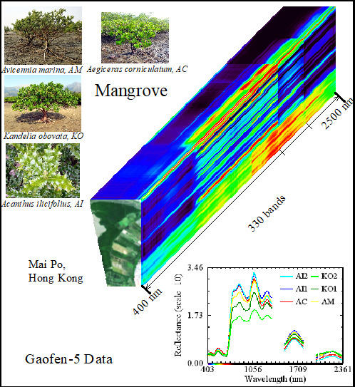
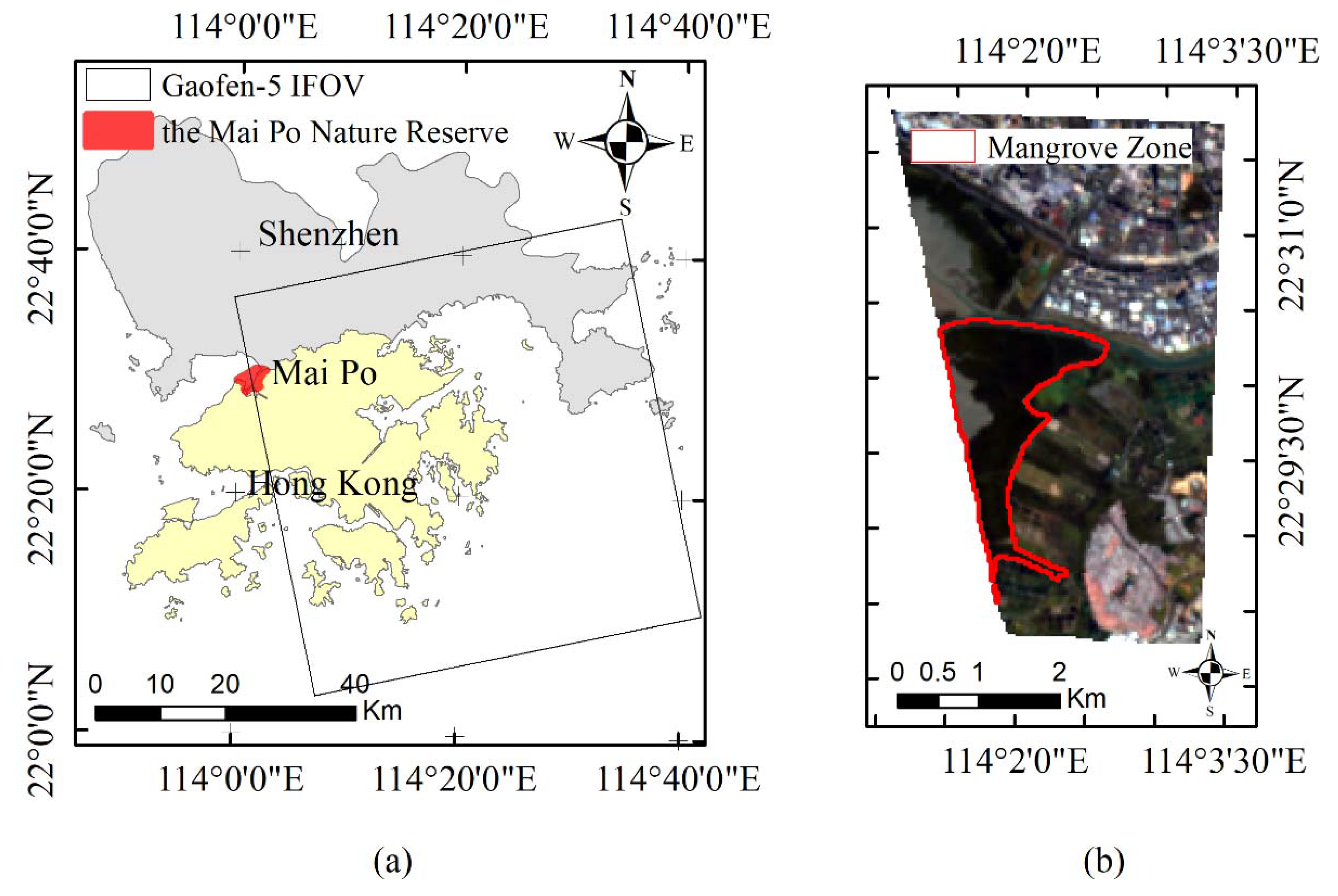
2.1. Study Site

The Mai Po Nature Reserve (MPNR, 113°59’E–114°03´E, 22°28´N–22°32´N) is located in the mouth of Shenzhen River, the northwest of Hong Kong, opposite to the Futian Nature Reserve, Shenzhen (Figure 1a). The reserve comprises of Geiwai, freshwater ponds, inter-tidal mudflats, mangroves, reed beds and fishponds, providing habitats for various wildlife (World Wild Fund for Nature - Hong Kong, WWF-HK 2016). Being a key station of the East Asian-Australasian Flyway (EAAF), it services million migratory birds every year. Due to the special location and significant eco-services provision, the reserve has been listed as restricted area via Wild Animals Protection Ordinance in 1975 and designated as a Site of Special Scientific Importance (SSSI) in 1976. In 1983, the nature reserve was developed and run by WWF-HK; it was further designated as a Ramsar Site in 1995.

The mangrove forest in the Mai Po is the largest one in Hong Kong with an area of around 319 ha [14], mainly occupying the core zone of the reserve. Six native and two exotic mangrove species have been found in the reserve. Specifically, Kandelia obovate (KO), Avicennia marina (AM), Aegiceras corniculatum (AC), and Acanthus ilicifolius (AI) are dominant, while Bruguiera gymnorrhiza and Excoecaria agallocha are less seen. It is believed that two exotic species including Sonneratia caseolaris and Sonneratia apetala are floating from the Futian Nature Reserve, and they are treated as invasive species and annually removed by Agriculture, Fisheries and Conservation Department (AFCD) due to potential threats to local species.

2.2. Dataset and Preprocessing

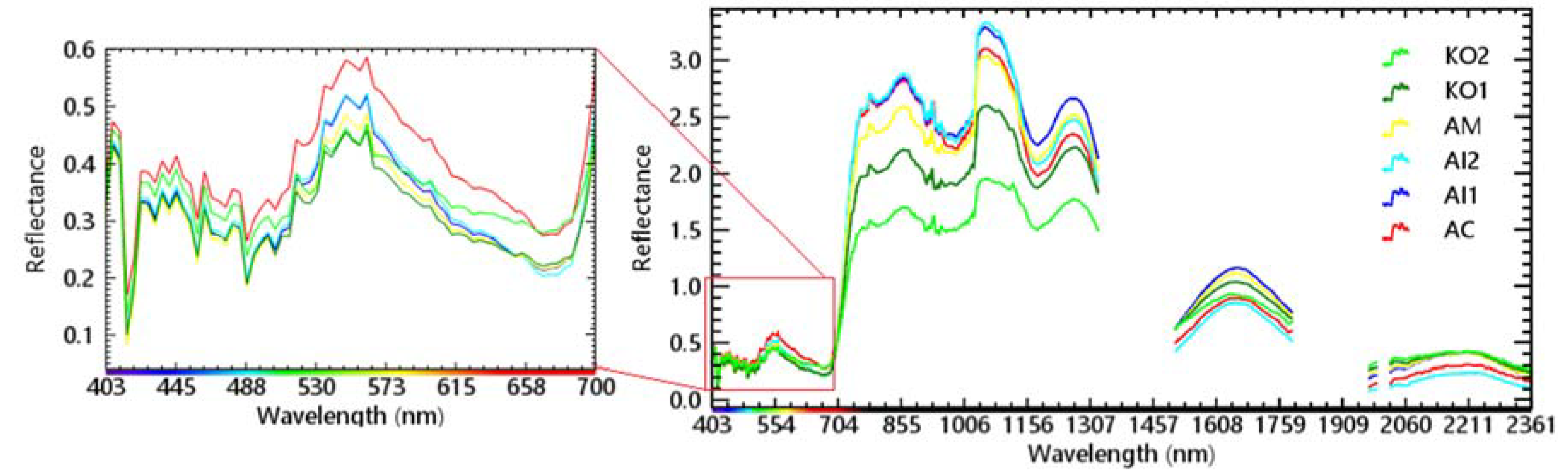
2.2.1. Hyperspectral Data and Preprocessing

The hyperspectral data adopted in this study was acquired by Advanced Hyperspectral Imager (AHSI) loaded by GF-5 satellite at 1:40 pm on 5 October, 2018. It provides Visible/Near-infrared (VNIR) and Shortwave infrared (SWIR) data with spectral range from 400–2500nm. Similar to Hyperion, the spatial resolution of GF-5 hyperspectral data is 30 m and the spectral resolution in SWIR is 10 nm. Due to the higher spectral resolution of 5 nm in VNIR, GF-5 hyperspectral data has double bands in VNIR and provides 330 bands in total (

Table 1. The characteristics of hyperspectral data from GF-5 satellite and Hyperion data.

Data	Band	Spectral Range (nm)	Spectral Resolution (nm)	Spatial Resolution (m)	Bands
GF-5	VNIR	390.324–1029.18	5	30	150
	SWIR	1004.77–2513.25	10	30	180
Hyperion	VNIR	355.59–1057.68	10	30	70
	SWIR	851.9–2577.08	10	30	172

).

The data was delivered as a Level 1 product, which has been preprocessed with radiometric calibration and noise removal by the China Centre for Resources Satellite Data and Application (CRESDA), China (http://www.cresda.com/). The radiometric calibration was conducted with a linear model with absolute coefficients calculated via laboratory experiments by CRESDA, China. After removing the bands without calibration or those contaminated by strips (

Table 2. Excluded bands of hyperspectral data from GF-5 satellite (* the absorption was referred to [28]).

Data Quality	Band N.O.	Bands
No Calibration	SWIR: 43–50, 96–112	25
Strip contamination	VNIR: 1–3; SWIR: 40–42, 51–60, 95, 113–115, 119–121, 163–180	41
Absorption*	VNIR: 128–132; SWIR: 15–19, 43–57, 96–115	45
Spectral Overlap in SWIR	SWIR: 1–4	4

), we conducted atmospheric correction using FLAASH module in ENVI 5.3.1 [28]. For the spectral overlap between VNIR (1006.68–1028.98nm) and SWIR (1004..57–1029.85nm), we kept the overlapped data in VNIR rather than SWIR to conserve accurate spectral information. Finally, we obtained 250 bands for GF-5 hyperspectral data (the details can be referred to the Appendix A).

To save the costs on computation, a region covering the MPNR maximumly was cropped from the Gaofen-5 hyperspectral image (Figure 1b), and fifteen ground control points were picked up from the cropped image for geometric correction with a result of Root Mean Square (RMS) of 0.048068. Because we focus on mangroves, the remaining objects like urban areas were firstly masked by manually outlining the initial region containing mangrove forests. The mudflat and water body were then removed from the initial region by thresholding Normalized Difference Vegetation Index (NDVI), which is calculated as a ratio between a red band around 660 nm and a near infrared band around 860 nm and widely used for primary separation vegetation from non-vegetation or mangrove from non-mangrove [32].

2.2.2. Field Survey and Sample Data

To investigate the real distribution of mangrove species in MPNR, a field survey was conducted along the floating bridge in the Mai Po on November 10, 2015. Based on the field survey, samples were manually identified with visual interpretation of a very high resolution WorldView-3 imagery with 1.6 m resolution in multispectral bands and 0.4 m resolution in the panchromatic band. Initially, 416 samples of six mangrove species containing the information on mangrove species and Global Positioning System (GPS) location were obtained [18]. To reduce the effect of the difference of date acquisition between hyperspectral data and samples on results, we identified the altered areas by comparing two very high spatial resolution images in two periods and removed the samples located in the changed areas. Finally, we added extra samples and obtained 293 samples of six classes (

Table 3. The description and sample number of six mangrove species collected in MPNR.

Species	Species Code	Description [6,33]	Sample Number (pixel)
Kandelia obovate	KO1	locate at the landward side, tend to be high	87
	KO2	locate at the seaward side; tend to be low	26
Avicennia marina	AM	locates in the central part of the Mai Po	70
Acanthus ilicifolius	AI1	locates at the landward side; tend to be with serrated leaves	49
	AI2	locates at the seaward side; tend to be with smooth leaves	42
Aegiceras corniculatum	AC	usually found as undergrowth	19

). In particular, AI was further divided into two subclasses (AI₁ and AI₂) according to whether leaves had smooth or serrated edges, and KO was also refined with two subsets of KO₁ and KO₂ according to the difference of tree height and leaf density [6,18,28], which may be related to the seaward or landward location [33]. Sonneratia was not selected as samples because of difficult percept of small patches from hyperspectral data after removal by AFCD. These samples were divided into training and testing samples with proportion of 70% and 30% respectively using the strategy of stratified random sampling. Based on the samples, the mean reflectance spectra of six mangrove species can be presented in Figure 2.

2.3. Methods

We designed a comparison experiment to assess the performance of GF-5 hyperspectral data in mangrove species mapping. Hyperion from EO-1 may be for benchmark since its global coverage with high quality and free charge. However, the available Hyperion covering the Mai Po is in 2008 and no more Hyperion data is provided after EO-1 decommission in 2017. The date difference of available Hyperion and Gaofen-5 hyperspectral data makes the comparison between them impossible. To overcome the limitation of available hyperspectral data for comparison with GF-5 hyperspectral data, we Simulated Hyperion (SH) data according to the spectral positions and bandwidth of Hyperion satellite based on GF-5 hyperspectral data with a simulation model. Besides, we also added another benchmark of Landsat 8 to be representative of multispectral data. Specifically, the Landsat 8 image closed to the date when GF-5 hyperspectral data was acquired and without cloud coverage was selected for comparison. The panchromatic band, cirrus band and thermal infrared bands were removed due to irrelevance to vegetation. Detailed experiment design is listed in

Table 4. The band number and bandwidth of five different datasets for comparison.

Data	Bandwidth (nm)	Bands
Landsat 81	430-450, 450-510, 530-590, 630-670, 850-880, 1570-1650, 2110-2290	7
Simulated Hyperion (SH)	The value of 1 in ‘Note’ field (See Appendix A)	144
SH + extra bands in VNIR of GF-5 (SH-GF5VN)	The value of 1 and 2 in ‘Note’ field (See Appendix A)	234
SH + extra bands in SWIR of GF-5 (SH-GF5SW)	The value of 1 and 3 in ‘Note’ field (See Appendix A)	160
GF5	403–929, 955–1029, 1038–1325, 1511–1788, 1974–1990, 2024–2361	250

¹ Landsat 8 was acquired on May 28, 2018.

.

2.3.1. Generation of Simulated Hyperion Data

EO-1 Hyperion data contains 242 bands, including VNIR of 70 bands and SWIR 172 bands, with spectral resolution of 10 nm and spatial resolution of 30 m. With same range from 400 to 2500 nm, GF-5 hyperspectral data has more bands since the spectral resolution was improved from 10 nm to 5 nm in VNIR. Regardless of the response difference for two spectra with an interval of less 5 nm, Hyperion can be viewed as the subset of GF-5 hyperspectral data. Consequently, simulating Hyperion from GF-5 can be regarded as the subset construction. Namely, the band of simulated Hyperion $b_i^{SH}$ with wavelength of i can be described with the band from GF-5 hyperspectral data ($b_j^{GF5}$) with wavelength of j if the difference between their wavelength is minimum and less than 5 nm, which can be formulated in Equation (1).

$$b_i^{SH}\approx b_j^{GF5}, \underset{j\in F}{\min }\left|j-i\right| where j\ne i and \left|j-i\right|<5$$

(1)

where F is the set of wavelengths of the valid bands from GF-5 hyperspectral data.

2.3.2. Mangrove Species Classification with Machine Learning Methods

More spectral features provided by Hyperspectral data make better performance possible. Meanwhile, they also promote a high requirement of classifiers due to high dimension [34,35]. Since this study aims to assess the efficiency of spectra, common approaches of dimension reduction, such as Principal Component Analysis (PCA) and Minimum Noise Fraction (MNF) will, because of their spectral characteristics, not apply to our purposes, because the contribution of the original spectral features cannot be tracked after applying the transformation from PCA or MNF. Therefore, the approaches which can inherently handle high-dimension features will be considered.

Random Forests adopts the principle of ensemble learning to vote the results from multiple weaker decision trees [36]. On the one hand, Random Forests randomly select a subset of features from all the features to split tree nodes, so they can deal with high-dimension features as well as maintain the robustness to noises. On the other hand, Random Forests randomly select a subset of samples from all the training samples to construct individual decision tree. When constructing a decision tree, around 63% of the samples are selected for training the tree while the rest (also named out-of-bag, OOB) for calculating an OOB error; and m features are randomly picked up from p features (total number of features). These m most distinguished features are selected for node splitting based on the measurement of Gini coefficient [37]. This procedure iterates until it reaches one of the stopping criteria, such as approaching maximum depth, minimum error threshold and maximum member of decision trees. Therefore, the tree number and feature number m are important for Random Forests construction. In principle, m was set to be $\sqrt{p}$ [38].

Support Vector Machine (SVM) is another approach which is not sensitive to feature dimension and well adapted to process hyperspectral data [39,40]. Based on structural risk minimization, SVM searches a hyperplane which can maximally separate two parts by projecting the data into a high-dimension linear space. For the case of nonlinearity, a kernel function is used to project the data into a higher dimensional space where the projected data become linearly distributed. Moreover, slack variable and penalty factors are introduced to control the bias and make them approximately separated. For the multiclass tasks of mapping multiple mangrove species, the “one-against-one” approach was used to construct many binary SVMs for each possible pair of two classes for training, while a voting strategy selected the class with maximum number of votes for classifying the new data. The details can be referred to in [41]. Kernel function has significant influence on the performance of SVM. In general, linear kernel and Radial Basis Function (RBF) kernel are widely used due to them having fewer parameter settings. We chose RBF for this study in consideration that linear kernel is a special case of RBF [42], for which the Gamma coefficient was set to be the reciprocal of dimension of input feature (HARRIS 2019).

2.3.3. Accuracy Assessment

Confusion matrix is employed to analyze the details on the classification of different classes over the samples, from which overall accuracy, Kappa coefficient, user accuracy and producer accuracy are derived for accuracy assessment in different aspects. In this study, we also adopted the overall accuracy and Kappa coefficient for accuracy assessment [43].

3. Results

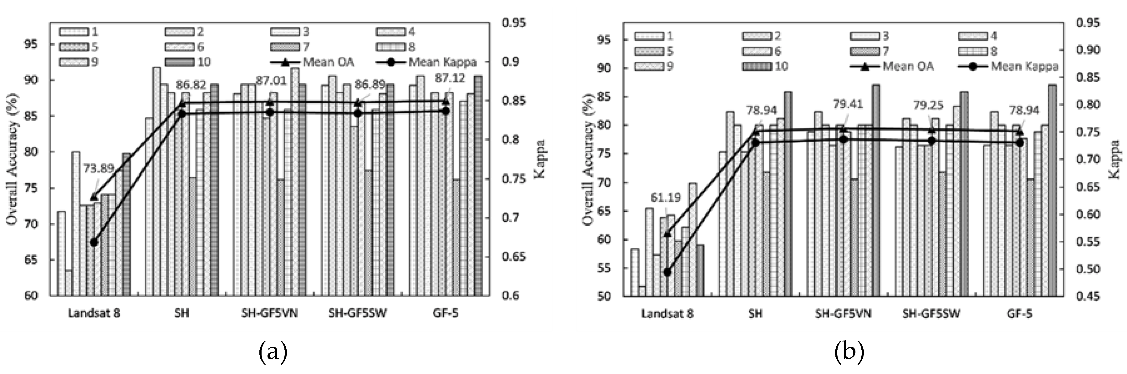
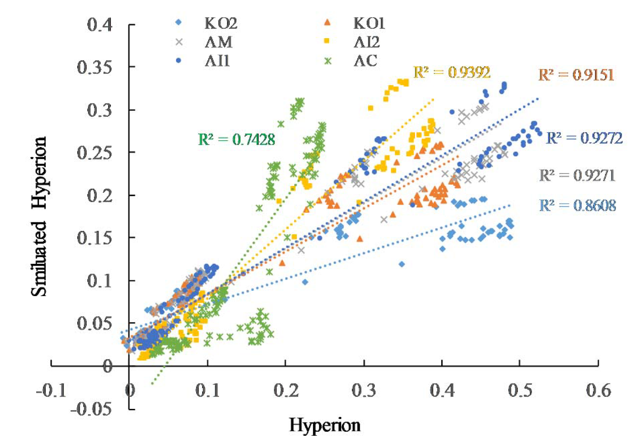
3.1. Comparison of Simulated Hyprion and GF-5

To better simulate the Hyperion, we adopted the valid bands from the available data acquired in 2008 [28] and got 153 bands for Hyperion. Due to sensors differences, nine bands with wavelength near 1336.87nm, 1346.97nm, 1488.29nm, 1498.4nm, 2002.8nm, 2012.9nm, 2375.98nm, 2386.08nm, 2396.18 nm are not available in GF-5 hyperspectral data. Therefore, 144 bands including 52 VNIR bands and 92 SWIR bands were simulated. Compared to simulated Hyperion, GF-5 hyperspectral data has nearly three times valid bands (142) in VNIR, while has 108 valid bands in SWIR. The details of simulated Hyperion can be seen in to the Appendix A.

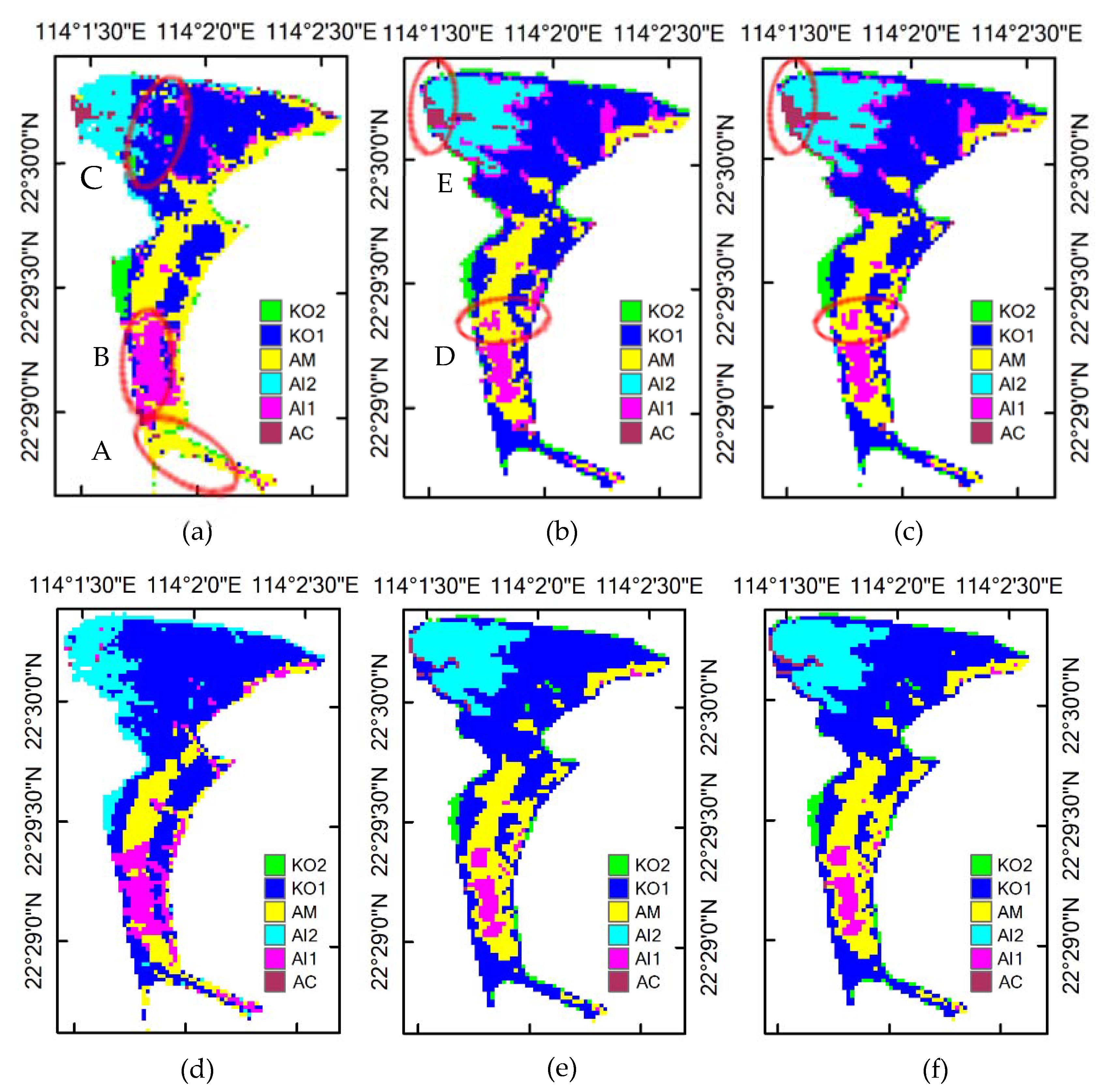
3.2. Mangrove Species Mapping with Accuracy Assessment

According to the data availability of GF-5 hyperspectral data and simulated Hyperion, the bands of experiment data including SH, SH-GF5VN, SH-GF5SW, GF-5 are 144, 234, 160 and 250 individually. Together with Landsat 8, these data are fed into both Random Forests and SVM for comparison. The number of decision trees for random forests was set 100, and the penalty factor for SVM with RBF kernel was set 100. To reduce the bias of sample division for training, we generated ten groups of training and testing samples through random selection with proportion of 70% and 30% respectively for ten times. As a result, we can obtain ten overall accuracies and mean overall accuracy for each dataset. The results using SVM and Random Forests can be seen from Figure 3.

Compared to multispectral data of Landsat 8, hyperspectral data including GF-5 and simulated Hyperion demonstrated significant advantage in mangrove species mapping with improvement in mean overall accuracy by 13%-17% and mean Kappa coefficient by 0.16-0.24 using two classifiers. Against simulated Hyperion, the increase in spectral resolution in VNIR (namely SH-GF5VN) or appended data in SWIR (SH-GF5SW) can make contribution to mangrove species mapping, showing growth of mean overall accuracy by 0.19% and 0.07% with Random Forests, while 0.47% and 0.31% with SVM. The mean Kappa coefficient of 0.835 over 0.834 (Random Forests) and 0.74 over 0.73 (SVM) for SH-GF5VN and SH-GF5SW also shows that the improvement from the increase in spectral resolution in VNIR is more significant than that from addictive bands in SWIR. Surprisingly, GF-5 hyperspectral, namely simultaneous enhancement in VNIR and SWIR based on simulated Hyperion, boosts further growth only with Random Forests, while it lowers the overall accuracy with SVM. The influence from classifiers on mangrove species mapping with remote sensing data can also be revealed from the comparison between Random Forests and SVM with same input data. In general, the overall accuracy resulted from Random Forests (Figure 3a) is higher than that resulted from SVM (Figure 3b) (73.89% VS 61.19%, 86.82% VS 78.94%, 87.01% VS 79.25%, 86.89% VS 79.25%, 87.12% VS 78.94%). Furthermore, we calculated the T-test between simulated Hyperion and GF-5 hyperspectral data, and the results show that the growth raised from the increase of spectral resolution in VNIR is not significant (

Table 5. The T-test of simulated Hyperion and GF-5.

P-Value (<0.05)	SH, SH-GF5VN	SH, SH-GF5SW	SH, GF-5
Random Forests	0.76283	0.91744	0.61711
SVM	0.37322	0.38491	0.99998

).

The average confusion matrixes for the classification with Landsat 8, SH, and SH-GF5VN were calculated for insight into influence of spectral resolution increasement on mangrove species mapping (

Table 6. The mean confusion matrix of mangrove species mapping using Random Forests with different datasets.

Data		KO2	KO1	AM	AI2	AI1	AC	Total	User Acc (%)
Landsat 8	unclassified	0.5	0.3	0	0	0	0	0.3
	KO2	5.9	0.2	0	0	0	0	6.1	96.72
	KO1	0	17.7	4.7	0.8	1.6	0.1	24.9	71.08
	AM	0	4.6	14.9	0.1	2.3	0	21.9	68.04
	AI2	0.3	0.6	0	10	0	1	11.9	84.03
	AI1	0	2.6	1.4	0	10.1	0	14.1	71.63
	AC	0	0	0	1	0	3.9	4.9	79.59
	Total	6.7	26	21	11.9	14	5	84.6
	Prod Acc (%)	88.06	68.08	70.95	84.03	72.14	78.00
SH	unclassified	0	0.3	0	0	0	0	0.3
	KO2	6.5	0.7	0	0	0	0	7.2	90.28
	KO1	0.5	22.1	1.3	0	0.4	0	24.3	90.95
	AM	0	2.9	18.3	0	2.2	0	23.4	78.21
	AI2	0	0	0	11.6	0	1.1	12.7	91.34
	AI1	0	0	1.4	0	11.4	0	12.8	89.06
	AC	0	0	0	0.4	0	3.9	4.3	90.70
	Total	7	26	21	12	14	5	85
	Prod Acc (%)	92.86	85.00	87.14	96.67	81.43	78.00
SH-GF5VN	unclassified	0	0.3	0	0	0	0	0.3
	KO2	6.3	0.6	0	0	0	0	6.9	91.30
	KO1	0.7	22.2	1.3	0	0.4	0	24.6	90.24
	AM	0	2.9	18	0	2.2	0	23.1	77.92
	AI2	0	0	0	11.6	0	0.7	12.3	94.31
	AI1	0	0	1.7	0	11.4	0.1	13.2	86.36
	AC	0	0	0	0.4	0	4.2	4.6	91.30
	Total	7	26	21	12	14	5	85
	Prod Acc (%)	90.00	85.38	85.71	96.67	81.43	84.00

). From the producer accuracy derived from Landsat 8, we can observe that KO₁ is difficult to be classify correctly with accuracy of 68.08%, and the confusion between AM and other species is serious with user accuracy of 68.04%, especially with KO₁. This situation will be improved with hyperspectral data (simulated Hyperion and SH-GF5VN), showing growth of around 17% and 10% in producer accuracy for KO₁ and user accuracy for AM. For the classification with simulated Hyperion and SH-GF5VN, the major difference comes from AC mapping. With the help of high spectral resolution in VNIR (SH-GF5VN), AC can be classified with higher accuracy of 84.00% against 78.00% from SH.

Visually, the misclassification and confusion can be also observed from the mapping (Figure 4). In the south part of study area (area A in Figure 4a), the majority of KO₁ was misclassified into AM, which is consistence with low producer accuracy of 68.08% in KO₁. In the area B where narrow zonation of AM was between AI₁ and KO₁, the confusion happens when using Landsat 8 (low user accuracy of 68.04%); while for area C, AI₁ and AM are confused. For the distribution of mangrove species resulting from simulated Hyperion and GF-5 hyperspectral data, they present a similar pattern with a minor difference in area D and E, where a small amount of AM was misclassified into AI₁ and more AC were correctly identified. Similarly, the results from SVM with datasets from Landsat 8 (Figure 4d), SH (Figure 4e) to SH-GF5VN (Figure 4f) show the major changes in AI₁ and AI₂. More specifically, the classification of AI₁ and AI₂ were refined with fine particles when using hyperspectral data (SH and SH-GF5VN). In contrast, fewer ACs were found from the mangrove species mapping using SVM, and KO located at the seaward side cannot be identified unless SH and SH-GF5VN are used.

Finally, we calculated the areas for each mangrove species in the study area using Random Forests with SH-GF5VN. The results show that the most dominant species is KO₁ with area of 103.95±3.56 ha (46% of the mangrove forests in the study area), followed by AM, AI₂, AI₁, and KO₂. The AC species are rare with an area of 6.93±1.07 ha, occupying only 3% of the mangrove forests in the study area. The details can be found in

Table 7. The areas of six mangrove species in the Mai Po estimated using Random Forests with SH-GF5VN.

Species	KO1	AM	AI2	AI1	KO2	AC
Area (ha)	103.95±3.56	45.15±2.87	34.28±1.82	22.42±2.23	14.36±1.02	6.93±1.07
Percentage (%)	46	20	15	10	6	3

.

4. Discussion

4.1. Quality Assessment of Simulated Hyprion

Simulated Hyperion based on GF-5 hyperspectral data is formulated by subset extraction, which hypothesizes that the deviation from two different sensors is minor for mangrove species mapping. To assess the quality of simulated Hyperion, we collected the spectral characteristics of six mangrove species based on shared samples which were picked up from the stable area without human interference in simulated Hyperion and true Hyperion data in 2008. Consequently, the spectral characteristics from two data sets should be similar with only a difference in growth, which can be viewed as intra-class variation. The correlation analysis of two spectra of six mangrove species indicates that it is reasonable to simulate Hyperion based on GF-5 hyperspectral data (Figure 5). Except for AC species, the Simulated Hyperion has low correlation with true Hyperion, which is possibly because AC grows at the outmost of mangrove forests where mixed pixels with mudflats are easily encountered. The reflectance of the rest simulated from GF-5 data is highly correlated with that of true Hyperion. Therefore, the Simulated Hyperion can be an alternative for comparison if Hyperion is not available.

4.2. Classifier Selection

According to the aforementioned findings, we learned that for the same input Random Forests outperform SVM if there is no feature selection. The contribution from extra minor information may be masked by abundant information due to high-dimension features with dependency when using SVM, which may explain the reason why further improvement was not expected with SVM but did with Random Forests. In another words, SVM may perform better with feature selection, which was also indicated in [39]. It should be noted that no feature selection was conducted in this study, because we did not aim for classifier optimization but for the contribution from the extra spectra on mangrove species mapping, and feature selection may lead to information loss.

4.3. Contribution of the Increase in Spectral Resolution in VNIR

We have learned from the confusion matrixes that the advantage of simulated Hyperion over Landsat 8 is to improve the accuracy of identification of many species including KO, AM, and AI, while, in contrast, simulated Hyperion GF-5 hyperspectral data shows metrics on the AC identification. From the Figure 2, we can see that the spectra of different species ranging from 403 nm to 740 nm (where most spectra of Landsat 8 lie) are similar. In contrast, most spectra from 780 nm to 1300 nm show distinguished differences. That is why the hyperspectral data (GF-5 and simulated Hyperion) can outperform Landsat 8 in mangrove species mapping with great improvement. In visible spectra, KO, AI and AC are with slight differences in reflectance, and the reflectance of AM lying between KO and AI are more similar to KO₁ and AI₁. This may explain the confusion of AM, KO₁ and AI₁ resulting in low accuracies in classification. In VNIR, KO has distinct features from others, and AM can be easily separated from one other with spectra ranging from 750 to 960nm, while AC and AI have similar spectra. This reveals that the increase in spectral resolution (from Landsat 8 to simulated Hyperion) can better discriminate mangrove species, and increasing the spectral resolution for hyperspectral data (from simulated Hyperion to GF-5 hyperspectral data) can better discriminate species with minor differences, which does make sense. The side effect of accuracy drop in KO and AM, which should have been easily separated with distinct features difference, is possibly because the introduced high-resolution spectra enlarge the intra-class variation for them. The similar problem of intra-class enlargement can be seen when increasing the spatial resolution. This may be resolved through individual processing by category, which was also used to exclude inter-class variation first to improve the results of mangrove biomass estimation [44]. This means that the effect of the additional spectra due to increase in spectral resolution should be explored in a new way.

4.4. Limitation of the Study

Due to a lack of true Hyperion data for comparison, a simulated Hyperion in this study was generated based on GF-5 hyperspectral in formulation of subset extraction. However, there is not always a solution for Equation (1). For example, the spectra in 1340–1520 nm for Hyperion cannot be simulated due to the differences of invalid bands between two sensors. The spectral loss (see Section 3.1 from simulated Hyperion should be analyzed, although there are only nine bands and they are close to the absorption windows of water vapor. Similarly, the work to which spectral features contribute most for one certain mangrove species should be analyzed. This may be useful for mangrove species discrimination in other sites. Another limitation is the sample number, especially for AC with small patches. More data will make the results more robust and convincing. Due to the small and narrow areas of each mangrove species, the GF-5 hyperspectral data with spatial resolution of 30 m cannot capture many pixels for each species, which makes it hard to collect more samples from the GF-5 hyperspectral data in the study area. Compared to the samples used in [6,14,18], we accepted the repeated use of our samples.

5. Conclusions

To date, GF-5 as the latest satellite which, in commission with hyperspectral data provision, offers potential opportunities for accurate observation due to higher spectral resolution in VNIR. In our study, we used GF-5 hyperspectral data for accurate mapping of mangroves in the Mai Po at species level. Our aim was to assess the performance of GF-5 hyperspectral data on mangrove species discrimination. We simulated Hyperion for the control hyperspectral data. Together with Landsat 8, various data with different spectral resolution is compared using Random Forests and SVM. According to the aforementioned results, we can draw the conclusions that follow.

1. GF-5 hyperspectral data can be used for accurately mapping six mangrove species in the Mai Po with accuracy of 87.12%;

2. GF-5 shows an advantage over Landsat 8 and Hyperion in mangrove species mapping due to an increase in spectral resolution in VNIR. Therefore, it is recommended to include more specific bands in VNIR for future satellites with the aims of mangrove species discrimination.

3. Extra spectra from GF-5 hyperspectral data with higher spectral resolution in VNIR acts on AC mapping;

4. Random Forests are preferred to SVM for mapping mangrove species when using GF-5 hyperspectral data without feature selection for spectral features.

References

1. Wang, L.; Jia, M.; Yin, D.; Tian, J. A review of remote sensing for mangrove forests: 1956–2018. Remote Sens. Environ. 2019, 231, 111223. [Google Scholar] [CrossRef]
2. Giri, C.; Ochieng, E.; Tieszen, L.L.; Zhu, Z.; Singh, A.; Loveland, T.; Masek, J.; Duke, N. Status and distribution of mangrove forests of the world using earth observation satellite data. Glob. Ecol. Biogeogr. 2011, 20, 154–159. [Google Scholar] [CrossRef]
3. Hamilton, S.E.; Casey, D. Creation of a high spatio-temporal resolution global database of continuous mangrove forest cover for the 21st century (CGMFC-21). Glob. Ecol. Biogeogr. 2016, 25, 729–738. [Google Scholar] [CrossRef]
4. Duke, N.C.; Meynecke, J.O.; Dittmann, S.; Ellison, A.M.; Anger, K.; Berger, U.; Cannicci, S.; Diele, K.; Ewel, K.C.; Field, C.D.; et al. A World Without Mangroves? Science 2007, 317, 41. [Google Scholar] [CrossRef] [Green Version]
5. Kovacs, J.M.; Wang, J.; Flores-Verdugo, F. Mapping mangrove leaf area index at the species level using IKONOS and LAI-2000 sensors for the Agua Brava Lagoon, Mexican Pacific. Estuar. Coast. Shelf Sci. 2005, 62, 377–384. [Google Scholar] [CrossRef]
6. Wang, T.; Zhang, H.S.; Lin, H.; Fang, C.Y. Textural-Spectral Feature-Based Species Classification of Mangroves in Mai Po Nature Reserve from Worldview-3 Imagery. Remote Sens. 2016, 8, 24. [Google Scholar] [CrossRef] [Green Version]
7. Fatoyinbo, T.; Feliciano, E.A.; Lagomasino, D.; Lee, S.K.; Trettin, C. Estimating mangrove aboveground biomass from airborne LiDAR data: A case study from the Zambezi River delta. Environ. Res. Lett. 2018, 13. [Google Scholar] [CrossRef] [Green Version]
8. Liu, M.; Zhang, H.; Lin, G.; Lin, H.; Tang, D. Zonation and Directional Dynamics of Mangrove Forests Derived from Time-Series Satellite Imagery in Mai Po, Hong Kong. Sustainability 2018, 10, 1913. [Google Scholar] [CrossRef] [Green Version]
9. Pham, T.D.; Yokoya, N.; Bui, D.T.; Yoshino, K.; Friess, D.A. Remote Sensing Approaches for Monitoring Mangrove Species, Structure, and Biomass: Opportunities and Challenges. Remote Sens. 2019, 11, 230. [Google Scholar] [CrossRef] [Green Version]
10. Yin, D.M.; Wang, L. Individual mangrove tree measurement using UAV-based LiDAR data: Possibilities and challenges. Remote Sens. Environ. 2019, 223, 34–49. [Google Scholar] [CrossRef]
11. Pham, T.D.; Bui, D.T.; Yoshino, K.; Le, N.N. Optimized rule-based logistic model tree algorithm for mapping mangrove species using ALOS PALSAR imagery and GIS in the tropical region. Environ. Earth Sci. 2018, 77. [Google Scholar] [CrossRef]
12. Zhang, H.; Li, J.; Wang, T.; Lin, H.; Zheng, Z.; Li, Y.; Lu, Y. A manifold learning approach to urban land cover classification with optical and radar data. Landsc. Urban Plan. 2018, 172, 11–24. [Google Scholar] [CrossRef]
13. Wang, L.; Sousa, W.P.; Gong, P. Integration of object-based and pixel-based classification for mapping mangroves with IKONOS imagery. Int. J. Remote Sens. 2004, 25, 5655–5668. [Google Scholar] [CrossRef]
14. Jia, M.M.; Zhang, Y.Z.; Wang, Z.M.; Song, K.S.; Ren, C.Y. Mapping the distribution of mangrove species in the Core Zone of Mai Po Marshes Nature Reserve, Hong Kong, using hyperspectral data and high-resolution data. Int. J. Appl. Earth Observ. Geoinf. 2014, 33, 226–231. [Google Scholar] [CrossRef]
15. Neukermans, G.; Dahdouh-Guebas, F.; Kairo, J.G.; Koedam, N. Mangrove species and stand mapping in GAzi bay (Kenya) using Quickbird satellite imagery. J. Spat. Sci. 2008, 53, 75–86. [Google Scholar] [CrossRef]
16. Wang, D.Z.; Wan, B.; Qiu, P.H.; Su, Y.J.; Guo, Q.H.; Wu, X.C. Artificial Mangrove Species Mapping Using Pleiades-1: An Evaluation of Pixel-Based and Object-Based Classifications with Selected Machine Learning Algorithms. Remote Sens. 2018, 10, 294. [Google Scholar] [CrossRef] [Green Version]
17. Viennois, G.; Proisy, C.; Feret, J.B.; Prosperi, J.; Sidik, F.; Suhardjono; Rahmania, R.; Longepe, N.; Germain, O.; Gaspar, P. Multitemporal Analysis of High-Spatial-Resolution Optical Satellite Imagery for Mangrove Species Mapping in Bali, Indonesia. IEEE J. Sel. Top. Appl. Earth Observ. Remote Sens. 2016, 9, 3680–3686. [Google Scholar] [CrossRef]
18. Wan, L.; Zhang, H.; Wang, T.; Li, G.; Lin, H. Mangrove Species Discrimination from Very High Resolution Imagery Using Gaussian Markov Random Field Model. Wetlands 2018, 38, 861–874. [Google Scholar] [CrossRef]
19. Kamal, M.; Phinn, S.; Johansen, K. Object-Based Approach for Multi-Scale Mangrove Composition Mapping Using Multi-Resolution Image Datasets. Remote Sens. 2015, 7, 4753–4783. [Google Scholar] [CrossRef] [Green Version]
20. Wang, L.; Sousa, W.P.; Gong, P.; Biging, G.S. Comparison of IKONOS and QuickBird images for mapping mangrove species on the Caribbean coast of Panama. Remote Sens. Environ. 2004, 91, 432–440. [Google Scholar] [CrossRef]
21. Vaiphasa, C.; Ongsomwang, S.; Vaiphasa, T.; Skidmore, A.K. Tropical mangrove species discrimination using hyperspectral data: A laboratory study. Estuar. Coast. Shelf Sci. 2005, 65, 371–379. [Google Scholar] [CrossRef]
22. Wang, L.; Sousa, W.P. Distinguishing mangrove species with laboratory measurements of hyperspectral leaf reflectance. Int. J. Remote Sens. 2009, 30, 1267–1281. [Google Scholar] [CrossRef]
23. Manjunath, K.R.; Kumar, T.; Kundu, N.; Panigrahy, S. Discrimination of mangrove species and mudflat classes using in situ hyperspectral data: A case study of Indian Sundarbans. Gisci. Remote Sens. 2013, 50, 400–417. [Google Scholar] [CrossRef]
24. Zhang, C.H.; Kovacs, J.M.; Liu, Y.L.; Flores-Verdugo, F.; Flores-de-Santiago, F. Separating Mangrove Species and Conditions Using Laboratory Hyperspectral Data: A Case Study of a Degraded Mangrove Forest of the Mexican Pacific. Remote Sens. 2014, 6, 11673–11688. [Google Scholar] [CrossRef] [Green Version]
25. Cao, J.J.; Liu, K.; Liu, L.; Zhu, Y.H.; Li, J.; He, Z. Identifying Mangrove Species Using Field Close-Range Snapshot Hyperspectral Imaging and Machine-Learning Techniques. Remote Sens. 2018, 10, 2047. [Google Scholar] [CrossRef] [Green Version]
26. Held, A.; Ticehurst, C.; Lymburner, L.; Williams, N. High resolution mapping of tropical mangrove ecosystems using hyperspectral and radar remote sensing. Int. J. Remote Sens. 2003, 24, 2739–2759. [Google Scholar] [CrossRef]
27. Chaube, N.R.; Lele, N.; Misra, A.; Murthy, T.V.R.; Manna, S.; Hazra, S.; Panda, M.; Samal, R.N. Mangrove species discrimination and health assessment using AVIRIS-NG hyperspectral data. Curr. Sci. 2019, 116, 1136–1142. [Google Scholar] [CrossRef]
28. Wong, K.K. Mangrove Species Mapping and Leaf Area Index Modeling Using Optical and Microwave Remote Sensing Technologies in Hong Kong. Phd, The Chinese University of Hong Kong, Hong Kong, 2012.
29. Koedsin, W.; Vaiphasa, C. Discrimination of Tropical Mangroves at the Species Level with EO-1 Hyperion Data. Remote Sens. 2013, 5, 3562. [Google Scholar] [CrossRef] [Green Version]
30. Krebs, G. Gaofen 5 (GF 5). Available online: https://space.skyrocket.de/doc_sdat/gf-5.htm (accessed on 23 December 2019).
31. Liu, Y.; Sun, D.; Hu, X.; Ye, X.; Li, Y.; Liu, S.; Cao, K.; Chai, M.; Zhou, W.; Zhang, J.; et al. The Advanced Hyperspectral Imager: Aboard China’s GaoFen-5 Satellite. IEEE Geosci. Remote Sens. Mag. 2019, 7, 23–32. [Google Scholar] [CrossRef]
32. Kuenzer, C.; Bluemel, A.; Gebhardt, S.; Quoc, T.V.; Dech, S. Remote Sensing of Mangrove Ecosystems: A Review. Remote Sens. 2011, 3, 878–928. [Google Scholar] [CrossRef] [Green Version]
33. Wong, F.K.; Fung, T. Combining EO-1 Hyperion and Envisat ASAR data for mangrove species classification in Mai Po Ramsar Site, Hong Kong. Int. J. Remote Sens. 2014, 35, 7828–7856. [Google Scholar] [CrossRef]
34. Tong, Q.; Zhang, B.; Zhang, L. Current progress of hyperspectral remote sensing in China. J. Remote Sens. 2016, 20, 689–707. [Google Scholar] [CrossRef]
35. Zhang, B. Advancement of hyperspectral image processing and information extraction. J. Remote Sens. 2016, 20, 1062–1090. [Google Scholar] [CrossRef]
36. Breiman, L. Random forests. Mach. Learn. 2001, 45, 5–32. [Google Scholar] [CrossRef] [Green Version]
37. Zhang, Y.Z.; Zhang, H.S.; Lin, H. Improving the impervious surface estimation with combined use of optical and SAR remote sensing images. Remote Sens. Environ. 2014, 141, 155–167. [Google Scholar] [CrossRef]
38. Liaw, A.; Wiener, M. Classification and regression by randomForest. R News 2002, 2, 18–22. [Google Scholar]
39. Cortes, C.; Vapnik, V. Support-vector networks. Mach. Learn. 1995, 20, 273–297. [Google Scholar] [CrossRef]
40. Pal, M.; Foody, G.M. Feature Selection for Classification of Hyperspectral Data by SVM. IEEE Trans. Geosci. Remote Sens. 2010, 48, 2297–2307. [Google Scholar] [CrossRef] [Green Version]
41. Chang, C.-C.; Lin, C.-J. LIBSVM: A library for support vector machines. ACM Trans. Intell. Syst. Technol. 2011, 2, 1–27. [Google Scholar] [CrossRef]
42. Hsu, C.-W.; Chang, C.-C.; Lin, C.-J. A Practical Guide to Support Vector Classification. Available online: https://www.csie.ntu.edu.tw/~cjlin/papers/guide/guide.pdf (accessed on 24 May 2019).
43. Congalton, R.G. Assessing Landsat Classification Accuracy Using Discrete Multivariate Analysis Statistical Techniques. Photogramm. Eng. Remote Sens. 1983, 49, 1671–1678. [Google Scholar]
44. Pham, L.T.H.; Brabyn, L. Monitoring mangrove biomass change in Vietnam using SPOT images and an object-based approach combined with machine learning algorithms. Isprs J. Photogramm. Remote Sens. 2017, 128, 86–97. [Google Scholar] [CrossRef]
Figure 1. The geographical location of the Mai Po Nature Reserve (MPNR, with red polygon) and Gaofen-5 instantaneous field of view (IFOV, in black rectangle) covering part of the Reserve (a), a scene of Gaofen-5 hyperspectral image was cropped to cover the Reserve (Red=698.166 nm, Green=544.196 nm, Blue=437.193 nm) and the mangrove zone was outlined with a red polygon (b).
Remotesensing 12 00656 g001
Figure 2. The mean reflectance spectra of six mangrove species (the scale was set to be 10 for demonstration).
Remotesensing 12 00656 g002
Figure 3. The overall accuracy of mangrove species mapping using Random Forests (a) and Support Vector Machine (SVM) (b) with different datasets and ten different groups of training and testing samples (number 1-10) through stratified random sampling with proportion of 70% and 30% respectively; the mean Overall Accuracy (OA) and mean Kappa coefficient were also shown in lines.
Remotesensing 12 00656 g003
Figure 4. Mangrove mapping using Random Forests with Landsat 8 (a), Simulated Hyperion (SH) (b) and SH-GF5VN (c), and the results using SVM with Landsat 8 (d), SH (e) and SH-GF5VN (f) were demonstrated for comparison.
Remotesensing 12 00656 g004
Figure 5. Correlation of reflectance from true Hyperion and Simulated Hyperion.
Remotesensing 12 00656 g005