Article

An Assessment of the GOCE High-Level Processing Facility (HPF) Released Global Geopotential Models with Regional Test Results in Turkey

Istanbul Technical University, Civil Engineering Faculty, Geomatics Engineering Department, Maslak 34469, Istanbul, Turkey
*
Author to whom correspondence should be addressed.
Remote Sens. 2020, 12(3), 586; https://doi.org/10.3390/rs12030586
Submission received: 23 December 2019 / Revised: 4 February 2020 / Accepted: 6 February 2020 / Published: 10 February 2020
(This article belongs to the Special Issue Remote Sensing by Satellite Gravimetry)

Abstract

:
The launch of dedicated satellite missions at the beginning of the 2000s led to significant improvement in the determination of Earth gravity field models. As a consequence of this progress, both the accuracies and the spatial resolutions of the global geopotential models increased. However, the spectral behaviors and the accuracies of the released models vary mainly depending on their computation strategies. These strategies are briefly explained in this article. Comprehensive quality assessment of the gravity field models by means of spectral and statistical analyses provides a comparison of the gravity field mapping accuracies of these models, as well as providing an understanding of their progress. The practical benefit of these assessments by means of choosing an optimal model with the highest accuracy and best resolution for a specific application is obvious for a broad range of geoscience applications, including geodesy and geophysics, that employ Earth gravity field parameters in their studies. From this perspective, this study aims to evaluate the GOCE High-Level Processing Facility geopotential models including recently published sixth releases using different validation methods recommended in the literature, and investigate their performances comparatively and in addition to some other models, such as GOCO05S, GOGRA04S and EGM2008. In addition to the validation statistics from various countries, the study specifically emphasizes the numerical test results in Turkey. It is concluded that the performance improves from the first generation RL01 models toward the final RL05 models, which were based on the entire mission data. This outcome was confirmed when the releases of different computation approaches were considered. The accuracies of the RL05 models were found to be similar to GOCO05S, GOGRA04S and even to RL06 versions but better than EGM2008, in their maximum expansion degrees. Regarding the results obtained from these tests using the GPS/leveling observations in Turkey, the contribution of the GOCE data to the models was significant, especially between the expansion degrees of 100 and 250. In the study, the tested geopotential models were also considered for detailed geoid modeling using the remove-compute-restore method. It was found that the best-fitting geopotential model with its optimal expansion degree (please see the definition of optimal degree in the article) improved the high-frequency regional geoid model accuracy by almost 15%.

Graphical Abstract

1. Introduction

The low-earth orbiting (LEO) satellite missions initiated a new stage in Earth gravity field studies and led to unprecedented progress in determining global gravitational field models and related parameters. In addition to the satellite laser ranging (SLR) tracking data, as a fundamental technique for gravity field determination since the earlier research [1], the recent contribution of the LEO satellites significantly improved global geopotential models (GGMs). The mentioned improvements are both in terms of precision and spatial resolution, and hence they can be assumed as a breakthrough with a stunning impact on geodetic science and related fields [2,3]. The observations by LEO satellites primarily rely on satellite-to-satellite tracking (SST), which includes high-to-low (hl-SST) as well as low-to-low SST (ll-SST) [4,5,6,7,8]. The fundamental principle of SST techniques is based on the precise measurements of distance variations between the satellites, which can be used to determine the orbit perturbations and hence the gravitational force acting on the satellite. In addition to SST, dedicated satellite gravity gradiometry (SGG), which is a sensitive detection technique of the space gravitational gradients, is also used in the LEO satellite technology and the gravitational field of the Earth is determined globally with high precision and resolution by means of combined SGG and SST observations.
As a chronological overview of the dedicated Earth gravity field satellite missions, the Challenging Minisatellite Payload (CHAMP), launched first, in July 2000 as a German Research Center for Geosciences (GFZ) project, and pioneered the LEO satellite missions for mapping the gravity field in a global scale. High-low SST with an equipped space-borne GPS-receiver on CHAMP enabled the determination of the long-wavelength static gravity field of Earth [9]. Thereafter, the Gravity Recovery and Climate Experiment (GRACE) twin satellites were launched in March 2002 as a US National Space Agency (NASA) and National Aeronautics and Space Research Center of Germany (DLR) joint project, aiming to track the changes in the gravity field initially for a five-year duration. The GRACE mission employed the dual-frequency one-way K-band phase measurements transmitted and received by both satellites [7,10]. Hence, precise mapping of the Earth’s gravity field with a 200–300 km half-wavelength resolution every 30 days was managed with the contribution of the mission data. Thus, many studies and applications in Earth science disciplines have benefited from the information relating to mass transport and redistribution in the Earth system by GRACE-based observations [11]. The science mission of GRACE ended in October 2017. As its successor, the Gravity Recovery and Climate Experiment Follow-On (GRACE-FO) mission was launched in May 2018 to extend GRACE’s observations and hence to continue its contribution to research [11,12].
Other than the GRACE and GRACE-FO missions, the Gravity field and steady-state Ocean Circulation Explorer (GOCE) was launched in March 2009 as a European Space Agency (ESA) project. The GOCE satellite mission utilized the satellite gravity gradiometer (SGG) for the first time in combination with the hl-SST technique. In addition to a novel SGG technique (see, e.g., [13,14]), with its low orbit altitude, the GOCE mission was dedicated to producing a near-global map of Earth’s static gravity field with high accuracy and resolution [5,8,15,16]. However, it should also be noted that considering the noise characteristics of the gradiometer, the SGG data alone are not sufficient to determine the low-degree harmonic coefficients of the gravity field with high accuracy. Therefore, the GPS SST data are essential to determine the precise orbit, and thus geo-locate the tensor observables, and the long-wavelength part of the gravity field. With the GOCE mission, an approximate 1–2 cm accuracy of geoid undulations and 1–2 mGal accuracy of gravity anomalies were targeted. An unprecedented spatial resolution of 100 km, which approximately corresponds to 200 degrees of spherical harmonic expansion, was accomplished in mapping the gravity field with the contribution of the GOCE satellite mission data [17].
A number of gravity field solutions were produced by the High-Level Processing Facility for GOCE (HPF) using the GOCE data. The official level 2 products of HPF can be obtained through datacenters such as the International Center of Global Earth Models (ICGEM) for GOCE users (geodesists, solid Earth scientists, oceanographers, etc.) [18,19,20,21].
In the released products, when the spherical harmonic expansion models (GGMs) are considered, it is seen that the maximum degrees of these models and hence their spectral contents vary in a rather large spectrum. Regarding the spectral bands, expressed by the maximum expansion degree, the GGMs can be classified as a low degree (having a degree/order (d/o) of harmonic expansion between 0 and 100), medium degree (100 < d/o ≤ 300), high-degree (300 < d/o ≤ 3000) and ultra-high degree (3000 < d/o) models (see, e.g., [15]). This described categorization of the GGMs is adopted in the present article.
This article aims to provide an overview of the geopotential models, particularly those released after the GOCE mission, in terms of the results of comprehensive quality validations using independent terrestrial data. The numerical tests include the GGM validations and their use in Turkey with the high-accuracy GPS/leveling data. These data include high order (first, second and third order) network quality GNSS coordinates (approximately 1–2 cm three-dimensional position accuracy) and orthometric heights (with ~2–3 cm accuracy) in the benchmarks. Turkey is one of the restricted areas in terms of terrestrial gravity field data sharing for global geopotential model calculations. As a consequence, the results of this study may be assumed to be a new statistical contribution to the literature on the model performance assessments of gravity field mapping using the recent HPF models in this territory. However, it should be emphasized that rather than suggesting a new methodology, it was aimed to demonstrate the performance gain of the geopotential models and to highlight the progress of HPF GOCE models from release to release, with the numerical assessment results using terrestrial data from Turkey. The impact of the improvement in geopotential model accuracies on the detailed geoid modeling in the area with rather sparse terrestrial gravity data was investigated as a second aim of this article. In summary, this article was written as a case study for providing a well-coordinated reference to users for geopotential model assessments, addressing the appropriate numerical methods that were suggested in the notable literature (i.e., spectral enhancement method or filtering the terrestrial data), rather than providing an innovative contribution to the theory.
The numerical validations of the GOCE- and GRACE-based geopotential models in the study area are accompanied by the high degree EGM2008 model. EGM2008, with 2190 d/o of spherical harmonic expansion, has been developed as a combination of the ITG-GRACE03S (complete to spherical harmonic d/o 180) geopotential model with the terrestrial, airborne and altimetry-derived gravity anomalies using least squares adjustment estimation technique. Reference [22] explains the computation method of EGM2008 in detail and reports the absolute accuracy of the model as ±5 cm to ±10 cm in well-covered areas with high-quality gravity data. Use of EGM2008 in the tests as the baseline model allowed an objective assessment of the level of improvement achieved by the GOCE mission, specifically at the low to middle frequencies of the gravity field spectrum, since this high-resolution model does not include the GOCE mission data. It should be noted that there is no official report that declares the terrestrial gravity or GPS/leveling data from Turkey that has been included in EGM2008 computation. The validation results in this study showed that the accuracy of EGM2008 ( = 2190 ) is at the decimeter level in Turkey.
In addition, EGM2008 has also been employed in this study for spectral enhancement of the validated GGMs for approximating the omission error in comparisons with the GPS/leveling data. The spectral content of the tested GGMs is naturally not comparable with the high-frequency GPS/leveling data. This is because of the truncated degrees in the spherical harmonic expansion equation. Recovering the omitted part of the signal, the spectral enhancement method (SEM) was applied. The SEM is one of the options that is given in the literature to overcome this handicap in validations [19,23]. Low-pass filtering of high-frequency data is another recommended option by [24,25,26]. In numerical tests, the short-wavelength components of the gravity field were taken into account by employing a high-frequency content of EGM2008 in addition to the residual terrain effect (RTE) from satellite-based high-resolution topographic data.
In the following section, the applied methods for validating internal and external accuracies of the tested GGMs, as well as for computing the detailed regional geoid models using the optimum and maximum d/o of the tested GGMs, are explained. A brief explanation of the main characteristics of the models is also provided in this section. The third section introduces the terrestrial data, which were employed in validations and regional geoid model computations. The numerical test results obtained from the validations of the GGMs, as well as the detailed geoid models, are provided using graphics and tables. Results are interpreted and discussed in this section. The fourth section summarizes the major outcomes of the study.

2. Materials and Methods

2.1. Practical Need of Global Geopotential Model Validation Results

Testing and evaluating geopotential model performances is important since determining an optimal model, with the highest accuracy and best resolution, has certain practical consequences in specific applications of the Earth science and engineering disciplines. We exemplify some of the applications in which GGM performance is crucial in the following by addressing the applied numerical tests under this study.
The determination of a high-resolution regional geoid using the remove–compute–restore (RCR) method combines low to high-frequency content of the gravity field signal employing the reference GGM, the terrestrial gravity observations and the topographic height and density data [27]. In this strategy, the best-fitting GGM to the gravity field in the region contributes to the accuracy of the high-resolution geoid by improving the long-wavelength component in the error budget [27,28,29]. The GGM contribution to the regional geoid model accuracy can be even more crucial if there is a lack of high-quality and sufficiently dense terrestrial gravity data under certain modifications of the kernel function and when a few-centimeter accuracy geoid model is desired (see e.g., [30]). Regarding this issue, we evaluated the released GGMs in high-frequency geoid computations using gravity data in Turkey. The computations were carried out with fast Fourier transform (FFT) evaluation of an unmodified Stokes integral. The conclusions depicted a centimeter-level contribution of the GGMs to the accuracy improvement of the regional geoid models.
The independent data provides an objective measure to examine the gravity field mapping performances of the GGMs in a region. Since the gravity field parameters and their gradients are directly estimated with spherical harmonic expansion equations in some applications, their accuracy checks are important. Regarding this, [31] uses the deflection of vertical (DoV) components estimated from GGMs to compare with the astrogeodetic DoVs obtained through the observations with the digital zenith camera system (DZCS); [32] exploits the GRACE-based GGMs derived gravity gradients in interpretation of geophysical or geodynamical patterns in Iran; [32] compares the upward continued airborne gravity data with the GOCE-based gravity gradients in Antarctica; and [33] issues the GGM-derived geoid heights and gravity anomalies to compare with the mean sea surface and free air anomalies derived from altimetry data in open ocean and coastal regions. In some GNSS applications, GGM-derived geoid undulations/height anomalies are considered for vertical control purposes. Before using the estimated undulations in the transformation of GNSS heights, the accuracies and the fit of the GGMs to the regional vertical datum should also be validated. For such a purpose, [34] evaluates five combined GGMs in a very dense GPS/leveling network on the Greece mainland and tested capability of parametric models for fitting the GGMs to the regional vertical datum.
The independent validations of the GGMs and test results are also important for the height system unification (HSU) and world height system (WHS) realization studies, because the precise determination of the offsets among the regional vertical datums, as well as with the WHS surface, is critical to establishing a globally unified height datum [23,35]. In this way, using a high-precision GGM as a reference in the calculations allows for higher accuracy calculation of regional height system offsets [35,36]. Although numerical assessments on the determination of the geopotential value (Wo) of regional vertical datum and height system unification are not explicitly undertaken in this article, [37] is recommended for further reading on the detailed numerical evaluations of a number of GGMs on the height system unification between Turkey and Greece.

2.2. Overview the Tested Global Geopotential Models

The tested GGMs in this study include the recent models that were calculated with different processing strategies from satellite orbits and GOCE gradiometer observations. These models were released (tagged with the release version from RL1 to RL5) as the products of the GOCE High-Level Processing Facility (HPF) of the ESA project. The first releases of the models (RL1) consist of the initial two months’ GOCE observations (between November 2009 and January 2010); the RL2 models are calculated employing the eight months’ observation cycle (November 2009 to July 2010); and the RL3, RL4 and RL5 releases exploit the 18 months, 26 months and the full mission observations, respectively [38]. The sixth releases of the direct and time-wise models, which were also based on the GOCE full mission dataset, were recently published and made available during the preparation of this article [21]. Therefore, the RL6 models were also employed and tested in the content of the study in order to compare their performances with the RL5 models, which have been already exploited the full mission observations.
Essentially, the models were developed according to three HPF gravity field processing approaches, namely, the direct (DIR) [39], time-wise (TIM) [40] and space-wise (SPW) [41] approaches. Each approach follows a different processing strategy in calculating the releases. These strategies include mathematical models, the adopted a priori models (or no a priori model use), reference information in constraints, spherical cap regularization, filter algorithms of the observations, etc. Table 1 provides a detailed comparison of the validated GGMs including a short report on the differences in their processing strategies. References [18,42] provide a detailed description of the basics of these data processing methods. Reference [18] reviews and discusses the DIR, TIM and SPW methods, their processing philosophies and architectures in computations of the GOCE gravity field models using RL1 models. Reference [16] reviews the second, third and fourth generation GOCE-based Earth gravity field models with their computation strategies, and evaluates their performances with spectral sensitivities over different functionals.
The products used in computations include gravity gradients in gradiometer reference frame (with identifier EGG_NOM_2), common-mode accelerations (EGG_CCD_2C), attitude quaternions (EGG_IAQ_2C), and precise science orbits (including the sub-products: kinematic orbits (SST_PKI_2I), variance–covariance information of orbit positions (SST_PCV_2I), reduced-dynamic orbits (SST_PRD_2I) and quaternions of transformation from Earth-fixed to inertial reference frame (SST_PRM_2I)); see [43] for the product descriptions and standards that were applied during the processes. In addition to the observations and products, depending on the applied processing strategy, the reference gravity field models were also adopted in some of the solutions. These reference gravity field models were either exploited as a priori information or for regularization, internal assessment and validation purposes. EIGEN5C, EIGEN51C, ITG-GRACE2010S [21] were used in the DIR method for internal validation purposes, whereas the GOCE quick-look gravity field model was used in the first release of the SPW approach as a priori information. EGM2008, EIGEN5C, EIGEN6C3stat were also employed for signal and error covariance computation in SPW solutions [21]. However, as the basic difference among the three methods, in the processing strategy of TIM method no gravity field a priori information entered the solution and, hence, this method yields pure GOCE-only models. All the information given here were retrieved from the headers of the spherical harmonic coefficients’ files and respective data sheets, published by [21]. The main characteristics of the models are summarized as follows:
The DIR method, as the classical approach, is based on the orbit perturbation theory and combines a priori orbits and an a priori gravity field model, hl-SST observations and common-mode accelerations, while constituting the normal equations in determining the gravity field model coefficients in an iterative way:
  • DIR models contain GRACE observations in the lower to medium degrees of the expansions (in addition to GOCE gravity gradient data).
  • As a priori gravity field information EIGEN5C (≤d/o 360) was introduced in DIR RL1, whereas the ITG-GRACE2010S (≤d/o 150) solution was the background model in RL2.
  • In RL3, RL4 and RL5 models, GRACE was combined with GOCE and SLR data on the basis of the normal equations (including the SLR data (LAGEOS-1 and -2)) in order to improve the gravity field solution, since the very low-degree harmonics (in particular degrees 2 and 3) cannot be estimated with GRACE and GOCE data).
  • In order to overcome the polar gap of GOCE’s observations caused by the orbit inclination of the satellite (inclined at 96.7° [18]), a spherical cap regularization (SCR) in accordance to [44] was applied using EIGEN-51C (≤d/o 240). In the later releases after RL1, the SCR was applied using GRACE and LAGEOS data. In the RL3, RL4, RL5 of DIR models, additionally, the predecessor release was used as a priori information (≤d/o 240, 260, 300, respectively, in the releases) and a Kaula regularization [44] was used beyond degrees 200 (for RL3, RL4) and 180 (for RL5).
  • In the DIR RL1 solution, the gravity tensor elements, which are measured with GOCE on-board SGG, were accumulated with the relative weights of Txx 1.0, Tyy 0.5 and Tzz 1.0. They were equally weighted in combination for the releases after RL1. In RL4, RL5 and RL6 models, the off-diagonal tensor elements Txz were also included.
  • In RL4 and RL5 models, the spectral bandwidth of the bandpass filter used to filter the SGG observations was extended by 1.7 MHz toward the lower frequency domain.
  • Reference [16] notes that contrary to the TIM approach, the DIR approach employs the GOCE gravity gradient information as restricted in a certain spectral band, which is close to the gradiometer measurement bandwidth (5–100 MHz [45]). However, the filtering procedure in the TIM approach allows the use of information on the gradient observations over the entire spectrum.
The TIM approach exclusively relies on an epoch-wise processing of GOCE SGG and hl-SST data according to the least squares principle. In the method, the SST data analysis is based on the kinematic orbit solutions with the energy integral approach (short-arc integral approach for TIM-RL4, RL5 and RL6). Hence, since TIM solutions are independent of any other gravity field information, they can be used for independent comparisons and combination with other satellite-only models (such as GRACE), terrestrial gravity data and altimetry data on the normal equations’ level. However, the TIM solutions are not competitive with the GRACE models in low degrees, since they are based solely on kinematic GOCE orbits but no external (such as GRACE) information:
  • The TIM models were constrained using Kaula’s rule regularization applied to (near-) zonal coefficients, improving the signal-to-noise ratio (constraints for high degree coefficients).
  • The off-diagonal tensor element Vxz was included in the models TIM RL3, RL4, RL5 and RL6. The stochastic models for the gravity gradient observations rely on optimum weighting based on variance component estimation.
  • TIM RL6e includes additional terrestrial gravity field observations over GRACE’s polar gap areas (>83° S, N) [46].
The revision in 2012 of the processing procedure of the Level-1b products led to the expectation of performance improvement of the GOCE’s SGG observations and consequently a quality improvement of the fourth, fifth and sixth releases of the models. Reference [47] reports that the gradiometry-only gravity field estimates show the largest improvement in recovery of low and medium degree coefficients, due to the new Level-1b products (see [16]).
In the SPW method, spatialized observations are produced from SST and SGG data using Wiener orbital filter [48] and the gravity field coefficients are derived by spherical harmonic analysis after transforming these observations into a spatial grid using least squares collocation [49]:
  • The SPW RL1 model includes the first GOCE quick-look model as the a priori information and the EGM2008 was used for error calibration of the estimated gravitational potential along the orbit that affects the low degrees of the solution. However, the later releases, RL2 and RL4, were not corrected using any a priori model, thus they are the GOCE-only models. EIGEN5C and EIGEN6C3stat models were respectively used in SPW RL2 and RL4 models’ computations for signal covariance modeling, in addition to FES2004 for ocean tide modeling.
  • In all SPW models, the off-diagonal tensor elements Vxz were included.
The maximum d/o of spherical harmonic expansion also changes (see the 2nd column of Table 1). The maximum d/o of the models was determined by the processing teams of HPF, depending on the signal-to-noise ratio, processing issues and the strategy of using additional a priori information [18].

2.3. Synthesis of the Gravity Field Parameters Using GGMs Spherical Harmonic Coefficients

The International Center for Global Earth Models [60] database has published 175 geopotential models so far and almost 30% of these models include GOCE mission data. In order to quantify the quality of the GGMs independently, validating the models using external information is necessary. So-called validations require the level-3 (L3) products from the satellite gravity missions to be compared with terrestrial data [24]. The GPS/leveling data is typically used for independent geoid undulations ( N G P S / l e v . ) at the benchmarks to compare with the GGM derived functionals ( N G G M ) using the following equation:
N G G M =   G M r γ = 2 m a x ( a r ) m = 0 ( Δ C ¯ m   c o s m λ   +   S ¯ m   s i n m λ   )   P ¯ m (   c o s θ )  
where (θ, λ, r) are co-latitude, longitude and geocentric radius of the computation point, respectively; a is the major axis radius of the reference ellipsoid; GM is the product of the gravitational constant and the mass of the Earth; and γ is the mean gravity of the reference ellipsoid. Δ C ¯ m = C ¯ m = C ¯ m C ¯ m e l l . , and S ¯ m are the fully normalized spherical harmonic coefficients, related to the normal potential of the reference ellipsoid from a specific degree of and order m (m = 0, 1, …,   ). The coefficients of the ellipsoidal normal potential ( C ¯ m e l l . ) contain only terms for order m = 0 (rotational symmetry) and degree = even (equatorial symmetry), and S ¯ m = S ¯ m . To calculate the normal potential in practice in most cases, it is sufficient to consider only the coefficients C ¯ 00 e l l . , C ¯ 20 e l l . , C ¯ 40 e l l . , C ¯ 60 e l l . and C ¯ 80 e l l . [20]. In the equation, P ¯ m ( c o s θ ) are the fully-normalized associated Legendre functions.
As can be seen, Equation (1) does not include the zero-degree geoid height term ( N o ), which is represented by the zero-degree harmonic coefficient in the spherical harmonic expansion model and means the position of the GGM geoid with respect to the geo-center of the Earth. The zero-degree term is expressed as depending on the difference between the constant (GM) value of the GGM and that of the reference ellipsoid ( G M G R S 80 ), which is GRS-80 for Turkey (see Equation (2)):
N o =   G M G M G R S 80 r   γ   W o     U o γ
where   U o corresponds to the normal gravity field of the GRS-80 reference ellipsoid with parameters of G M G R S 80 = 398 , 600.50 × 10 9   m 3 / s 2 ; thus, it is U o = 62 , 636 , 860.85   m 2 / s 2 [61]. Using r = 6378.137   km and γ = 981   Gal , the zero-degree geoid height (considering solely the first component at the right-hand side of Equation (2)) corresponds to the N o =   0.936   m that is to be added to the N G G M , derived from Equation (1). The residual zonal-coefficients (shown as Δ C ¯ m in Equation (1)) account for the difference between the reference radius of the GGM and the semi-major axis of the GRS-80 ellipsoid [62,63]. In the synthesis of GGMs’ spherical harmonic coefficients, the zero-degree term is considered either by taking the zero-degree zonal-harmonic coefficients (as C ¯ 00 = 1.0 ,   S ¯ 00   does   not   exist ,   C ¯ 10 = 0.0 ,   S ¯ 1 m = 0.0 ) into account via initiating the computation from the = 0 or otherwise separately adding the zero-degree geoid offset, calculated with Equation (2). The second component at the right-hand side of Equation (2), ( W o U o γ ), introduces the difference between the gravity potential of the geoid ( W o ) and the normal gravity potential on the surface of the normal ellipsoid ( U o ). In the ideal case, without irregularities of topographic densities, the two potentials are equal ( W o =   U o ). As a primary parameter for the definition of the reference (zero-height) surface with respect to Earth’s body (which provides an absolute definition to the vertical datum of a height system), a global estimation of W o is required [64].
In addition to the zero-degree term definition, another issue in the synthesis of the gravity field parameters from the GGMs’ spherical harmonic coefficients is adopting the proper permanent tide-system to which the GGMs’ functionals refer. The permanent tide-systems, commonly adopted in studies investigating Earth dynamics include mean-tide, zero-tide and tide-free [65]. In studies related to the Earth’s potential field, investigations of the Earth’s crust deformations or determination of the best-fitting ellipsoid to the geoid, a proper permanent tide system is adopted. According to Bruns’ definition of geoid undulation [61], the geoid undulation changes from one tide system to another depending on the geometric change in the shape of the geoid (but with a constant W =   W o potential for each tide-system) relative to a fixed reference ellipsoid [65]. In other words, the W o value does not change among the systems, but the shape of the geoid changes. The effect of changing the permanent tide-system is defined basically with the second-degree zonal harmonic coefficient C ¯ 20 [65].
In this study, the gravity field parameters were synthesized using the GGM coefficients in a tide-free system. In order to have comparable geoid undulations at the GNSS/leveling benchmarks, the orthometric heights in regional vertical datum were converted from the mean-tide to tide-free system according to following the equation [66]:
H t i d e   f r e e = H m e a n   t i d e 0.68   ( 0.099   0.296   s i n 2 φ )

2.4. Assessments of the Global Geopotential Models Using Spectral Enhancement Method (SEM)

The spectral constituents of Earth’s gravity field are denoted with the spectral bands of a GGM [15]. The gravity field quantities as observed on the Earth’s surface contain the full spectral signal power, while any global geopotential model is limited by its spectral resolution, which leads to omission error in the output functional. When comparing GGMs with independent observational data, one should take into account spectral incompatibility of both data sets. To overcome the spectral band limitation of the mode, the so-called spectral enhancement method (SEM) is suggested and applied by [18]. The fundamental principle of the SEM is based on bridging the spectral gap between the GOCE-based GGM functional and ground-truth data, using the relevant auxiliary data set (such as a higher resolution geopotential model like EGM2008, and the residual terrain data, to account for the ultra-high frequencies) as much as possible. Hence, the ground-truth data for validation purposes are approximated much better, and thus the influences of omission error on the comparison results are consequently minimized. In spectral enhancement, the GGM, expanded to a spherical harmonic degree 1 (e.g., 1 = 240 for DIR_RL1), is enhanced using the spectral bands over the degrees of ( 1 + 1 ) until 2 from a higher resolution Earth geopotential model (e.g., 2 = 2190 when using EGM2008). The very short-wavelength components of the gravity field, represented with spectral bands beyond degree 2 (e.g., 2 = 2190 in our case) until the maximum possible degree (e.g., 216,000), are completed as the residual terrain effect (RTE) of topographic data on the estimated geoid heights (see Equation (4)).
N e n h .   =   N o + [ N | 1 2 + N | 2 1 + 1   ] +   N R T E | 216000 2 + 1
Equation (4) is a symbolic representation of the enhancement procedure in terms of geoid undulation derived using the GGM, where N o is zero-degree geoid undulation; [ N | 1 2 + N | 2 1 + 1   ] is the geoid undulation calculated with enhanced coefficients according to Equation (1). Here, N RTE is the residual terrain effect on geoid undulation, calculated using the digital topographic data [27]. As the summation of the components that represent each different spectral constituent of the Earth’s gravity field, the full spectral content geoid undulation ( N e n h . ), which is comparable with ground truth data, is obtained.
In Equation (4), N R T E was calculated using the residual terrain model (RTM) mass reduction method evaluated in the Gravsoft program package, following the processing methodology outlined by [27], Section 8.4.4 Terrain Effects and High Resolution Global Geopotential Models in pp. 366–371. In computations, 3 arc-second Shuttle Radar Topography Mission (SRTM) topographic data was used for approximating the real terrain and the spherical harmonic expansion of the DTM2006.0 (up to d/o 2190) was used to model the mean elevation surface [27].

2.5. Spectral Analysis of GGMs

In the assessment of the quality of the GGM solutions, two types of errors are defined. Firstly, the noise in the observations that are used in the calculation of the GGM coefficients propagates from the measurements to the solutions, which is called the commission error. Secondly, an error is revealed because of estimating the projection of the gravity field functional (taking the anomalous potential as an example) on the finite dimensional subspace (generated by linear combinations of solid spherical harmonics up to a limited degree) instead of deriving its full content. This error is known as the omission error. The omission error has an easy formulation that is set by considering the coefficients left out from the truncated convergent series. In fact, this is the sum of the squares of all coefficients of degree higher than m a x . Clearly, however, this is an unknown quantity, which cannot be known a priori. However, the so-called degree variances (i.e., the sum over all orders of the squares of the coefficients up to a certain degree) can provide an idea of the GGMs’ signal decay, which allows one to judge the commission error and compute the omission error according to an adopted law [27]. Accordingly, the signal and error degree variances of the GGMs provide an insight into the omission/commission error content of a GGM under consideration (see [24]). Hence, they are regarded as internal error estimates for the investigated models.
Using the fully normalized spherical harmonic coefficients, C ¯ m , S ¯ m from a specific degree of m a x and order m (m = 0, 1,…   m a x ), the signal degree amplitudes (or square root of power per degree ) of functions of the disturbing potential T ( φ ,   λ ,   R ) at the Earth’s surface are computed as follows [20,21,27]:
σ = m = 0 ( C ¯ m 2 + S ¯ m 2 )
Equation (5) provides the signal degree amplitude σ in terms of unitless coefficients, and the σ ( N ) in terms of geoid heights (meter) is shown in Equation (6):
σ ( N )   = R   σ
The error spectra of GGMs are investigated depending on the error degree amplitudes, calculated using the estimation errors of the Stokes’ coefficients ( σ C ¯ m ,   σ S ¯ m ) of a spherical expansion model:
σ c ( N )   =   R   m = 0 ( σ C ¯ m 2 + σ S ¯ m 2 )
As a function of minimum and maximum degrees , the accumulated (signal, error) degree amplitudes provide the power spectrum accumulated over a spectral band (between 1 —usually 1 = 0   or   2 as minimum degree of the expansion—and 2—usually 2 = m a x as the maximum degree of the harmonic expansion equation) and shows the increase in overall power with increasing degree of :
σ 1 2 ( a c c u m u l a t e d )   = = 1 2 σ 2

2.6. GGMs’ Contribution in High-resolution Regional Geoid Modeling

For the determination of high-resolution precise regional gravity field models, remove–compute–restore (RCR) is a very well-known approach and has been used in calculation of many countries’ geoid models to date [27,61]. In the RCR scheme the terrestrial gravity and topography/bathymetry data are used along with a global geopotential model to smooth the observations for data gridding, transformations, predictions and to eliminate the aliasing effects [27]. The computation steps of the RCR procedure are as follows:
Δ g r e s = Δ g F A Δ g G G M   Δ g t c
Equation (9) represents the ‘remove’ step where the long-wavelength component ( Δ g G G M , from the GGM according to Equation (10)) of the gravity field, as well as the short-wavelength components ( Δ g t c , the direct topographical effect on gravity, which consists of the subtraction of the attraction of condensed topographic masses from the attraction of all topographic masses above the geoid and is calculated as according to a selected reduction scheme—i.e., Helmert’s Second Method of Condensation was used in this study (see Equations (3–97) of Section 3.9 in [61])—using topographic data), are removed from the free-air gravity anomalies ( Δ g F A ). Hence the calculated and reduced residual gravity anomalies ( Δ g r e s ) on the geoid surface are evaluated in Stokes’ formula.
Δ g G G M =   G M r 2 = 2 m a x ( 1 ) m = 0 ( Δ C ¯ m c o s m λ + S ¯ m s i n m λ   )   P ¯ m (   c o s θ )  
where the terms in Equation (10) are as introduced previously in Equation (1).
The ‘compute’ step includes the computation of the residual co-geoid using Stokes’ integral ( N Δ g ), the long-wavelength geoid undulation ( N G G M ) using the GGM according to Equation (1) and finally the indirect effect of topographic mass attraction on geoid undulation ( N i n d using topographic data according to Equation (13)). After computing all constituents separately, their compilation step is called ‘restore’ and formulated as follows:
N =   N G G M + N Δ g   +   N i n d  
as the high-resolution geoid undulation ( N ).
The Stokes’ formula for calculating N Δ g is:
N Δ g =   R 4 π γ σ S ( ψ ) Δ g r e s d σ
where σ is the surface element, R is the mean Earth radius and S ( ψ ) is Stokes’ function having the angular distance ψ from the computation point to the differential surface element d σ . N i n d is:
N i n d = π   G ρ H Q 2 γ   G ρ R 2 6 γ σ ( H Q 3 H P 3 ) s 3 d σ
where ρ is the density of topographic masses; H Q and H P are the heights of the running and computation points, respectively; and s is the planar distance between P and Q. Hence, the output of the equation is N i n d according to Helmert’s Second Method of Condensation reduction scheme [27]. The details of the computation steps followed in this study were explained in [28] pp. 433–435 and Figure 13 given in the cited reference illustrated the adopted computational schema in here.
In the computation of a regional geoid model with hybrid (mixed) data in RCR, the GGM is responsible for the long-wavelength (signal) error content (see Equations (10) and (11)). When calculating a geoid model over a spatially limited region, while having low-accuracy and sparse terrestrial data, the quality of the GGM becomes even more important to compensate for the weakness of the terrestrial data accordingly in the RCR algorithm with specific modifications [30,67].

3. Results and Discussion

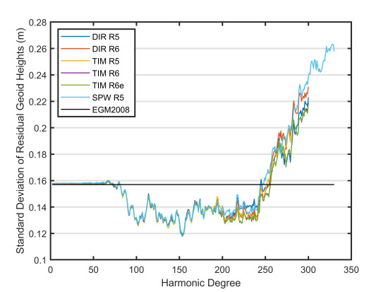
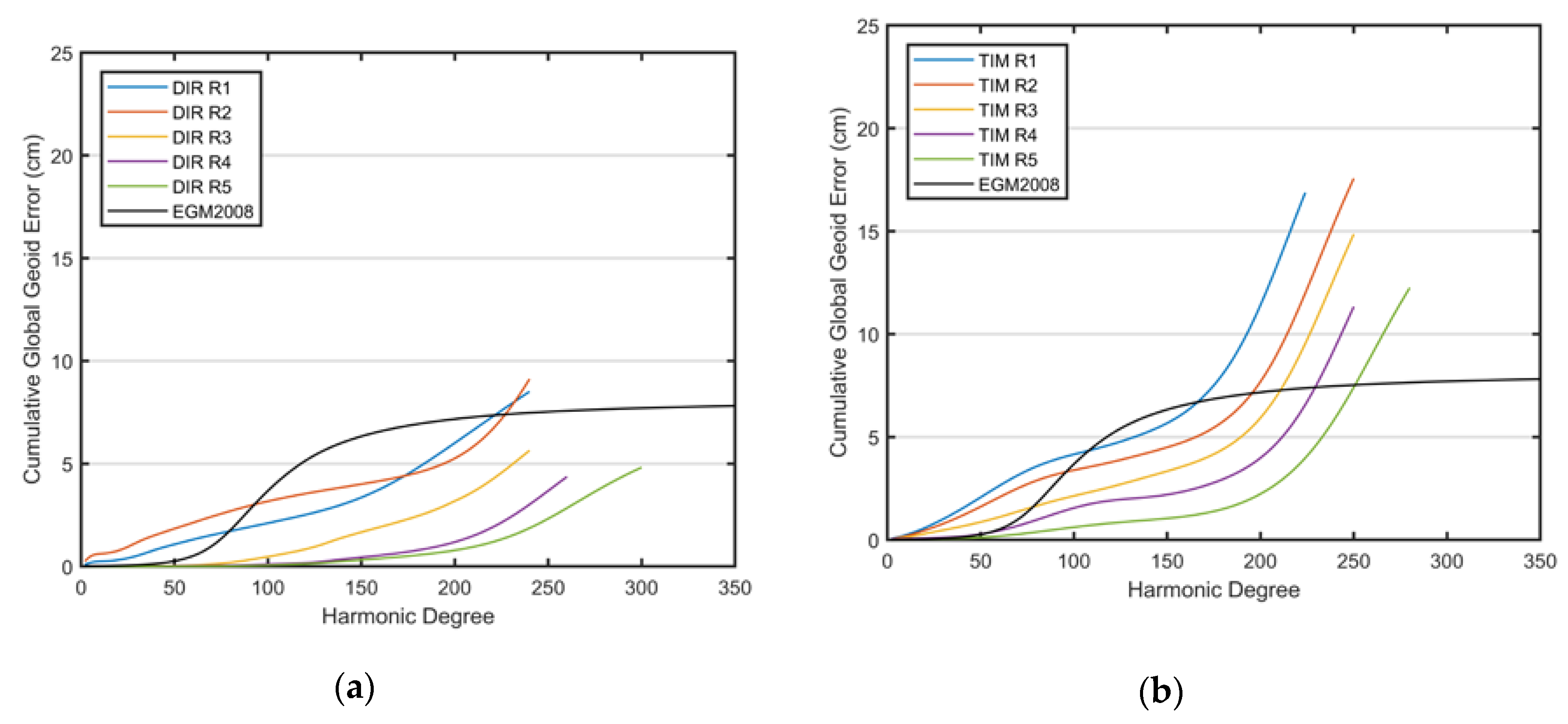
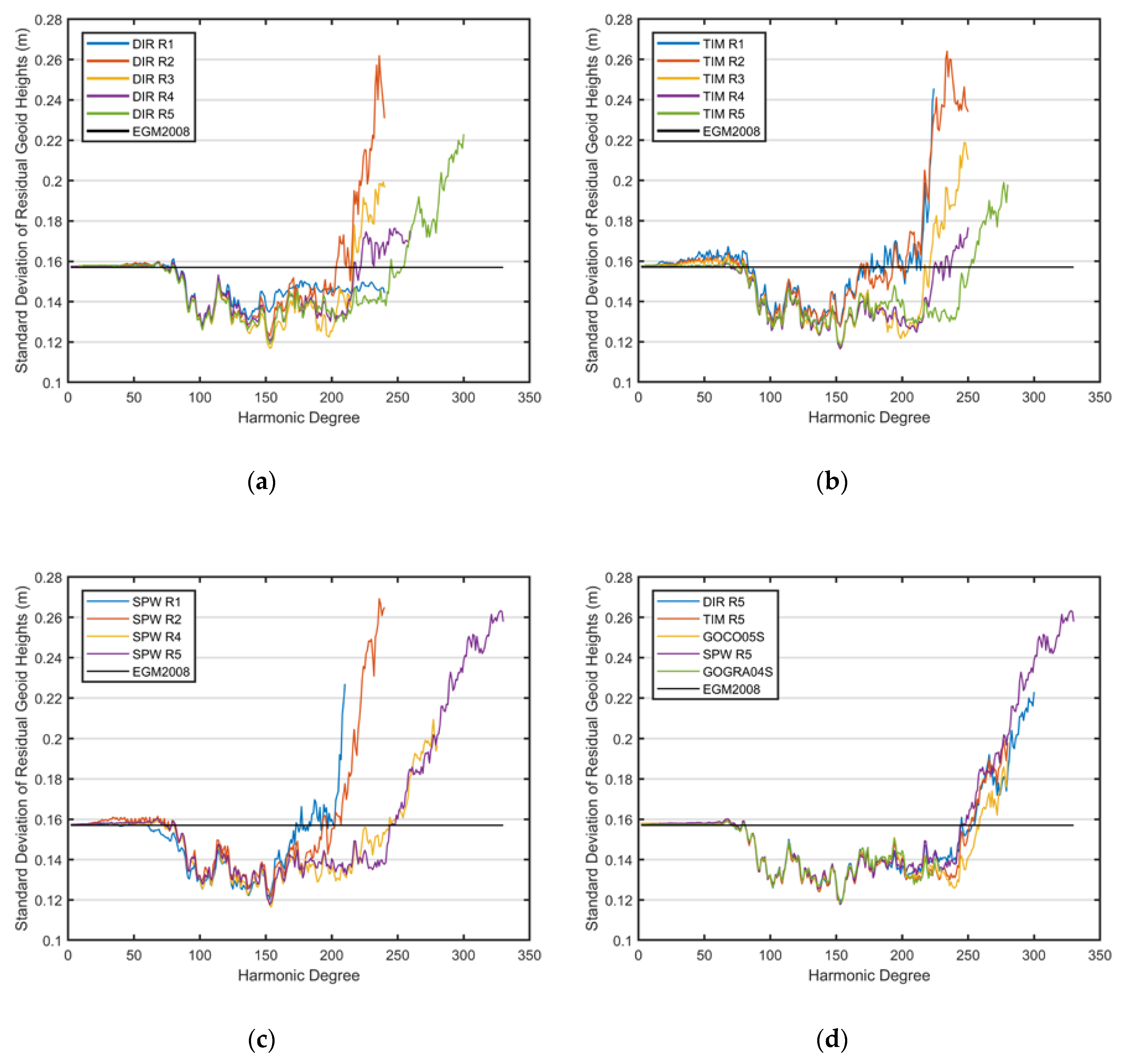
3.1. Internal Error Estimates of Tested GGMs

The error degree variances of the tested models were considered for internal uncertainty estimates of the GGMs. The theory and formulations for calculating error degree variances were given in Section 2.5. (see Equations (7) and (8)). Figure 1 shows the degree-wise accumulated error amplitudes of the models. The figures reveal the overall geoid undulation accuracies up to the maximum degree of each model. For d/o 200, which corresponds to the spatial resolution of 100 km, the cumulative errors are 0.8 cm for the DIR RL5 model (see Figure 1a), 2.2 cm for the TIM RL5 model (Figure 1b), 2.7 cm for the SPW RL4 model (Figure 1c), 2.0 cm for the GOCO05S model and 2.9 cm for the GOGRA04S model (Figure 1d), whereas it is 7.1 cm for the EGM2008 model, in terms of geoid undulation.
When the cumulative error amplitudes are investigated, it is seen that the improvement with the final releases of the GGMs is up to 80% compared to their predecessors. It is also noteworthy that the cumulative error estimates of TIM RL5 and DIR RL5 differ by a factor of three. However, it is arguable if these cumulative error estimates depending on degree variances are realistic and, on the other hand, whether calibration is required or not. In this manner, in a similar study on GGM validations, [51] suggests applying a calibration factor of two for the DIR RL5 model.
Related to concerns about the uncertainty estimates of the GGMs depending on the error degree variances approach, [68] emphasizes these issues: (1) firstly, the correlations among the coefficients are ignored while evaluating the GGMs with degree variances; (2) the effect of the polar-gap problem on the zonal and near-zonal coefficients of the GOCE-only models obviously influences the provided standard deviations of the spherical harmonic coefficients, specifically for the GOCE-only TIM and SPW models; and (3), on the other hand, dependence of the GOCE models’ uncertainties and performances on the geographic location cannot be ignored in evaluations. Regarding the mentioned handicaps, beside the degree variances-based assessments, evaluating the GGMs using geographically dependent standard deviations (if possible) with the propagation of full variance–covariance matrices of the spherical harmonic coefficients is suggested by [68].
In summary, although the accumulated error degree variances provide a global mean of the GGM’s performance over the entire sphere, which is significantly influenced by the large uncertainties in the polar gap, deriving concluding measures for its performance in a local region is not straightforward. Therefore, Section 3.2 provides results of local validations of tested GGMs using terrestrial data.

3.2. Overview of the Regional Accuracies of the GGMs

The results of evaluating the gravity field models using various data sets in different regions are being published regularly as the new models are released. However, the methodologies applied in these assessments vary to differing degrees. Regarding a number of significant studies from the literature, the following can be noted.
Reference [19] provides a detailed assessment of the first generation GOCE-based models using LEO satellite orbit perturbations and GPS/leveling geoid height differences. The conclusions of their study confirm that the orbital perturbations are mostly sensitive to the long-wavelengths of the gravity signal and hence provide clear results in quality assessments of the GGMs in a global manner. In contrast, the geoid comparisons using GPS/leveling data give the opportunity to assess the model performances at the medium to short-wavelengths. In the study, the regional assessments using the GPS/leveling data were carried out in Australia, Europe, North America (US and Canada), Japan and Germany. The preliminary conclusions from this study give a global geoid accuracy of about 5–6 cm with a 111 km spatial resolution (at d/o of 180). Here, it is emphasized that they obtain this level of accuracy as a result of just two-month GOCE data, and the goal of the mission (1–2 cm geoid accuracy with 100 km resolution) could be reached with the availability of more data. In terms of geoid residual RMS values, [19] reports the EGM2008 model accuracies as the most improved in Germany (3.5 cm), Japan (10 cm) and Canada (10.5 cm), whereas weaker fitting performances were found in Australia (24 cm), Europe (21.5 cm) and the US (26.5 cm) with comparatively larger residual RMS values. The non-homogeneous control datasets and vertical datum distortions were cited as possible reasons for the larger error levels in the continent-wide assessments.
Reference [21] provides the validation statistics of the released model for the maximum truncation degrees (without spectral enhancement) using similar datasets. Reference [15] evaluated the first generation GOCE-based models globally using EGM2008 and regionally using terrestrial gravity data and astrogeodetic vertical deflections. The analyses by [15] clearly show the improvement in gravity field mapping with GOCE data contribution and identify the reasons for the reported improvement specifically at certain spectral bands. Reference [69] evaluated the first and second releases of the models by means of gravity anomalies and radial gradients from GOCE gradiometer data using least squares collocation at several regions. The evaluations of the models from the first to third releases were published by [70] using the terrestrial gravity data in Norway and [71] over the Earth by means of gravity gradients from the GOCE gradiometer data. There are also other studies that validate the GOCE-based GGMs over different regions using various terrestrial data sets including [72] (in Sudan), [73] (in Brazil), [74] (in Hungary) and [68] (in Germany). Reference [75] provides the recent results of regional validations of all releases over different countries. However, the literature lacks information by means of GGM validation statistics over many areas of Earth. This may stem from the countries’ data restriction policies and/or lack of quality terrestrial data for the region. Accordingly, the numerical section of this study focused on regional evaluation of the GGMs in Turkey.
In the following sections, in addition to reporting the models’ formal error estimates, the performances of the GOCE-based GGMs were evaluated in terms of absolute accuracies. The GOCE-based models were compared with EGM2008 in order to clarify the GOCE observations’ contribution to the GPS/leveling benchmarks in Turkey. In addition, the spectral bands of the spherical harmonic expansion models, where the improvement of tested GGM is the most significant, were determined and employed in the regional geoid modeling.

3.2.1. Assessment of GGMs’ Accuracies in Turkey

In accuracy assessments of the HPF-released GGMs in Turkey, a number of numerical tests were carried out in the country at 36°N–42°N latitude and 26°E–45°E longitudes. The test statistics of the geoid height residuals ( Δ N ) of the observations and the models were calculated for two different high order GPS/leveling network benchmarks, separately. The GPS/leveling networks include 30 and 81 points, respectively. The first dataset covers the whole of Turkey (Dataset I), and the latter is denser but localized in the northwest of the country (Dataset II) [76]. Carrying out the tests individually using both datasets (instead of using a unified dataset) aims to make validation results independent from the effects of possible datum differences between the datasets. A detailed description of the employed data is provided in Table 2. The distributions of the benchmarks on the topographic maps are given in Figure 2 and Figure 3.
The numerical results of the study were interpreted from different perspectives, including: (1) verifying the role of the data amount and the calculation strategy of the model on its accuracy and performance; (2) determining an optimum d/o of the models available in the study area (whereas the term of the “optimum” possibly sounds vague and its definition is dependent on the application, the “optimum d/o” was used here to mean the degree of the spherical harmonic expansion at which the highest accuracy is obtained in the tests performed with the terrestrial data in the study area); and, (3) clarifying the contribution of a best-fitting geopotential model with its optimum d/o to the development of a precise regional geoid model using RCR approach.
In the following, Figure 4a and Figure 5a show the evaluation results of the DIR RL1, RL2, RL3, RL4 and RL5 models, which are enhanced using the high-resolution EGM2008 model and high-resolution DTM data (SRTM3), at GPS/leveling networks with 30 benchmarks throughout Turkey and 81 benchmarks in the northwest of the country, separately. The graphics show the standard deviations of the geoid height residuals, calculated at the co-located GPS/leveling benchmarks with the GGM-derived geoid undulations, which were truncated and enhanced degree by degree from two to the maximum harmonic expansion d/o of the tested models (see Equations (1) and (4)). Looking at the statistics of the two datasets in the graphics, the improvement of the model performances from the first release to the last can be verified.
Similarly, Figure 4b and Figure 5b show the performances of the TIM models, depending on the standard deviations of the geoid undulation residuals at co-located GPS/leveling benchmarks. Considering the results in graphics, the improvement of the TIM models as the release number increases is also clear.
The SPW models were also compared for the given two geodetic network datasets in Figure 4c and Figure 5c. The statistics of SPW model validations also show the progress with increasing release number.
The numerical tests, which were carried out fulfilling the first objective of the current section, show improvement in the models with the increasing amount of data (by means of the observation cycle; please see Table 1). This conclusion has been drawn independently from the GGM computation strategy. Carefully looking at the graphics given in Figure 4 and Figure 5, the direct models reveal almost similar performances to each other and with the EGM2008 model, of up to approximately 70 d/o of the spherical harmonic expansions; however, this is not the case for the TIM and SPW models. This situation can be explained as a consequence of the differences among their computation strategies (compare the strategies and the a priori information in computations in Table 1). Since EIGEN-51C combined GGM [39] was employed for the regularization of the GOCE-based models in the direct approach, they were reinforced by this background model. In the long-wavelengths, the used background model utilizes the information from GRACE and CHAMP, and the medium to short-wavelengths are provided by DNSC08GRA [77] and thus (indirectly) the terrestrial gravity (as contained by EGM2008) over the land areas. Regarding the information on the determination of the direct models, it is not possible to strictly quantify which spectral bands provide improvement, and the extent to which improvement is provided by the GOCE observations when considering solely these models.
The processing strategy for computation of the time-wise models relies exclusively on GOCE gradiometry and hl-SST observations, and only Kaula’s regularization is employed to constrain the model at the short-wavelengths. Hence, the assessments of time-wise models can provide a realistic measure of the GOCE-based contribution to the GGMs without the intervention of other data sets. When the evaluation results of these models are considered, the contribution of the GOCE signal to the improvement of gravity field mapping in Turkey is clarified (see Figure 4b and Figure 5b). The maximum improvement is seen at the spectral bands between d/o 100 and 250 as is promised by the GOCE Earth gravity field satellite mission.
The improvement in gravity field mapping with a GOCE-based contribution is shown to be significant in Figure 5. However, it is not highly significant in the test results obtained with 30 benchmarks, distributed over the country (see Figure 4). This may be because of the insufficient density and distribution of the test benchmarks (as seen in Figure 1) and relatively lower accuracy of the GPS/leveling heights at these benchmarks. Hence, it may be concluded that the first dataset, with 30 benchmarks, is not sufficient by means of data quality and distribution for carrying out a detailed assessment of the geopotential models regarding different spectral bands. However, the evaluation results using this data set were nonetheless considered as a country-wide look at the accuracy level of the tested GGMs. In this manner, the test results that were obtained through the locally distributed 81 benchmarks (Dataset II) revealed the significant improvement of the GOCE-based models in the medium-wavelength spectral bands.
Considering the entire statistics from the evaluations of direct, time-wise and space-wise models (namely, GO_CONS_GCF_2_ DIR, TIM, SPW) for the two datasets, it is concluded that the computation strategy of the GGMs does not have a significant role in the improvement of the model accuracies. In this part of the study, in addition to the GOCE-based DIR, TIM and SPW models (actually computed with the contribution of the GOCE and GRACE missions’ data), the final releases of the two other combined GGMs, namely, the GOGRA04S and GOCO05S models, were also evaluated. The GOGRA04S model combined approximately four years of GOCE gradiometry data with GRACE observations from a cycle of satellite tracking in excess of 10 years. Despite the complementary advantage of the two missions in the solution, the GOGRA04S model did not reveal significant improvement in mapping the regional gravity field compared to the last releases of the GOCE models (see graphics in Figure 4d). The GOCO05S model combined four years of GOCE gradiometry data with GRACE, CHAMP and SLR observations (with the GRACE normal equations from the ITSG-GRACE2014S model). In the assessment results, the performance of the model is better than that of GOGRA04S and almost equal to the final releases of the GOCE-only models up to d/o of 155 and, in relative assessment, it performs better than the other models for degrees between 230 and 270 (Figure 4d and Figure 5d).
Accordingly, the accuracies of the GGMs in terms of standard deviations of the geoid height residuals, obtained through their maximum and optimum degrees (optimum degree corresponds to spherical harmonic expansion degree of the model with the highest accuracy with a minimum standard deviation of the geoid undulation differences; see Figure 5), are shown in Figure 6a,b, separately computed for each test area, respectively. Given statistics in figures are derived using the enhanced coefficients of the GGMs over optimum (blue bars) and maximum (orange bars) expansion degrees of the models using the EGM2008 model and high-resolution DTM. The accuracies that are obtained through employing the full-expansion of the EGM2008 model are shown with a black color bar at the end of each graphic.
The given statistics show that the GGMs, enhanced on their optimum d/o, revealed an almost 50% better fit comparing the results obtained from the enhanced models on their maximum degrees. Comparing with the EGM2008 model, the maximum improvement was recorded by the SPW RL5 model (a 23.8% improvement with respect to the EGM2008 model) in the test results using the second data set. Regarding the overall test results, obtained using both datasets, separately, it was seen that the GOCE-based GGMs had accuracies between 10 cm and 15 cm in Turkey. While interpreting the reasons for obtaining different fitting statistics of the GGMs in the tests with two datasets, it is worth noting the possible role of the tectonic structure in the region. Turkey is in the collision zone between three plates (African, Arabian and Eurasian) (see [78] for the active faults in Turkey) and hence continuously exposes horizontal and vertical crustal movements (see [79,80] for vertical and horizontal velocities in Turkey). Accordingly, the approximate rates in horizontal and vertical positions are reported as 2–3 cm/year in [80]. Moreover, an earthquake of Mw ≥ 6 occurs every 1–2 years, particularly around the North Anatolian Fault Zone. All these activities continuously distort the geodetic networks by time and even have a minor effect on the change of the gravity field; however, the latter is not significant for the scope of this study. Hence, the first geodetic network (Dataset I) was exposed to the Izmit earthquake of 1999 (7.6 Mw) and the northwest part of this geodetic network, including the 81 benchmarks of Dataset II, have been remeasured and adjusted since then. Although the networks were positioned at the same geodetic datum, the physical establishments of the network stations were distorted by time and these distortions negatively influence their quality as control data in model evaluations. As a conclusion, the ground-truth data employed to validate the qualities and fitting performances of the GGMs should be of high quality, sufficiently dense, homogeneously distributed over the test area and as up-to-date as possible, especially in areas under the influence of dynamic Earth activities, such as Turkey.
In addition, the recently published sixth releases of the direct and time-wise models were considered in evaluations and they were compared with the RL5 models by means of standard deviations of the geoid undulations at the second dataset benchmarks. Figure 7 shows the comparisons of the models. According to obtained statistics, the RL6 models shown similar performances with the RL5 models between the 100 and 200 d/o of the spectrum. However, in degrees between 200 and 280, TIM RL6 models shown slightly better performance comparing with the RL5 and DIR RL6 models and had an improvement in standard deviation less than 1 cm.

3.2.2. Testing the GGMs Contribution in Detailed Geoid Modeling

A high-resolution geoid model has been an essential component of the modern geodetic infrastructure in many countries, particularly in recent decades (see the geoid models’ repository at [81] for some of the released regional geoid models). As a consequence of the progress in global positioning systems, many countries, such as Canada, New Zealand and the US, redefined their vertical datum to refer to a precise geoid model utilizing GNSS techniques. Hence, they also aimed to obtain further benefit from the satellite-based positioning technology for obtaining precise physical point heights in real time in many geodetic applications. Equations (11)–(13) provide the fundamental theory in the determination of a high-resolution geoid model using RCR steps. As was seen, the method combines GOCE-based GGM data with terrestrial data. Thus, the error content of the geoid undulation (Equation (11)) includes the errors from the global geopotential model, as well as the terrestrial gravity data and digital height data. Therefore, in order to clarify how the GGM accuracy affects the determination of the high-resolution geoid model, the numerical results from regional geoid modeling studies in Turkey are shared and discussed in this article. The terrestrial gravity data used in the RCR computations of this study are in five arc-minute resolution gravity anomalies in the IGSN-71 datum. Reference [82] reports that the estimated accuracy of the used gravity anomaly grid is at the level of 7–8 mGal based on cross-validations, as well as validations using point-wise gravity observations.
Using the terrestrial gravity data and the identical computation parameters, twelve experimental detailed geoid models (expTG-) were calculated for Turkey. Each of these models relies on a different GGM with either the optimum ( o p t = 155 ) (called expTG-Opt models) or the maximum (called expTG-M models, having m a x = 330 / 300 / 280 ) degrees of the spherical harmonic expansions. In the tests, in addition to the best performing DIR RL5, TIM RL5, SPW RL5 and GOCO05S models, the EGM2008 coefficients up to the identical expansion degrees ( m a x = 155 ,   280 ,   300 ,   330 ) of the other tested models were also considered (see the test statistics of the experimental models in Table 3).
The twelve experimental models were validated at 81 GPS/leveling benchmarks of the geodetic network in northwest Turkey. Regarding the obtained results (see Table 3), all the validated experimental geoid models (relying on the reference GGM with optimum d/o of spherical harmonic expansion) provided an accuracy of 16.5 cm in terms of standard deviations of the residual geoid undulations without removing the tilt/trend at GPS/leveling benchmarks. However, employing the GGMs with the maximum degrees of their expansions, the calculated experimental geoid models revealed an accuracy of approximately 20 cm. This means that the use of optimum d/o of the geopotential model led to an improvement in the accuracy of the regional geoid model using Stokes’ integral without any modification and any cap size limitation. The table also includes the statistics of the experimental geoid models after de-trending the models’ surface simply using a third-order polynomial equation. The cross-validation of the de-trended models gave a so-called improved accuracy of around 9.7 cm for the models. The expTG-Opt-1 geoid model surface is shown in Figure 8.
As also seen in Table 3 (statistics before fit), the detailed geoid models, which were calculated using the classical RCR algorithm with GOCE-based reference models, are not more accurate than the enhanced EGM2008 model. This is a consequence of insufficient accuracy and density of the mean terrestrial gravity anomalies that were used in the computations. The role of the terrestrial gravity data accuracy for the quality of the calculated geoid model is explained by [83,84]. In accordance with a 1–2 mGal accuracy of the terrestrial gravity data, having 1–2 km spatial resolution with homogenous distribution is required if 1–2 cm accuracy of the geoid undulations is aimed. Compared to this criterion, the accuracy and resolution of the used mean gravity anomalies (with 6 mGal accuracy and 5′ grid spacing) in computations do not satisfy the requirements for determining a centimeter accuracy regional geoid. The accuracy of the used GPS/leveling data (~1.5–2.0 cm three-dimensional position accuracy and ~2.0 cm leveling height accuracy) in validations was sufficient for the purpose of this study. Although it is not officially declared in technical reports explaining the calculation strategy and data content of EGM2008, if the terrestrial gravity data of Turkey or the surrounding area was used in EGM2008 computations, this could explain the superior performance of this model in the validation results.
It is possible to obtain slightly improved accuracy in regional geoid models by applying modifications to the Stokes’ integral in order to achieve a more rigorous combination of the geopotential models with terrestrial data by also considering their variances [38]. Hence, it will be possible to compensate for the random errors that are contained in the terrestrial data with the improved quality of the geopotential models up to a certain amount.

4. Conclusions

The purpose of this study is to investigate the progress of GOCE High-Level Processing Facility (HPF) released geopotential models that include data from gravity field satellite missions, and provide assessment results of these models for Turkey. The analyses were carried out by means of both spectral and spatial approaches. Regarding the numerical results and obtained statistics through these analyses, the following conclusions were drawn:
GOCE HPF-released GOCE- and GRACE-based global geopotential models were validated using the cumulative degree variances. Regarding the spherical harmonic expansion degrees (between 100 and 200 degrees of SH expansions, corresponding to the medium-wavelengths of the gravity field, where a significant contribution of the GOCE mission is expected), the cumulative formal errors (in terms of the geoid undulations) were 0.8 cm, 2.2 cm and 2.7 cm for DIR RL5, TIM RL5 and SPW RL4 models, respectively, whereas they were 2.0 cm, 2.9 cm and 7.1 cm for GOCO05S, GOGRA04S and EGM2008 models, respectively.
Considering the cumulative error amplitudes at the corresponding degrees for 100 km spatial resolution, the significant improvement toward the final releases of the geopotential models was verified (the improvement of final releases is almost up to 80% with respect to the first releases). On the other hand, the cumulative formal error estimate of the TIM RL5 model is three times worse than that of the DIR5 model. Though the difference seems to be quite significant, it is arguable if such a comparison without any calibration is objective.
The regional validations of the tested geopotential models against the GPS/leveling data were carried out with the spectral enhancement method. Hence, the higher frequencies in the content of the tested GGMs were synthesized from ultra-high degree coefficients of the EGM2008 model and the regional DTM data. As a conclusion, the spectral enhancement method revealed meaningful results and is recommended to be used for GGM validations using terrestrial data. In the results of the comparisons among the model releases (in every group of models as DIR, TIM, SPW), it is concluded that the model accuracy improves as its release increases, and that this improvement is independent of the computation strategy.
The spatial analyses of GGMs were carried out using GPS/leveling data of high-order geodetic networks in Turkey. The accuracy of the used control data, their spatial distribution and density, as well as the size of the validation area, are critical for the model validations and affect the reported performances. In this manner, the second test dataset can be said to be more suitable and hence the obtained validation statistics are more realistic in terms of the detailed analyses of the GGMs in the study area. The spatial analyses results clarified the GOCE mission’s contribution to the improvement of the GGMs (with respect to the EGM2008 model), especially in the corresponding spectral bands of 100 and 250 degrees. Moreover, comparing standard deviations of the geoid undulation differences calculated with an increasing degree of the spherical harmonic expansion model, the optimum degree was determined with a minimum standard deviation value. Accordingly, the optimal value for d/o of spherical harmonic expansion is around 155 in the study area. In the test results explained in Section 3.2.1, an approximate accuracy for the tested GGMs is about 12 cm. EGM2008 model accuracy is calculated to be around 15 cm in Turkey. This is three times greater than the reported absolute accuracy of this model for well-covered areas with quality terrestrial data on Earth. This result indicates that either EGM2008 does not include the terrestrial data of Turkey or the quality of the included data is low. In the analyses, the GOGRA04S and GOCO05S models were also validated. However, since the obtained statistics did not reveal any improvement, it can be concluded that the complementary advantage of the GOCE gradiometry data with the observations from other gravity field satellite missions and SLR is not significant.
In the final part of the study, the role of the reference geopotential model accuracy, as well as its optimal expansion degree in determination of the detailed hybrid geoid model, were validated based on the RCR computation algorithm.
The obtained results revealed a 15% improvement in the accuracy of the gravimetric geoid model (considering the results without corrector surface fitting) when the GGM is employed with its optimum degree instead of the maximum degree (~16.5 cm vs. 19.5 cm for DIR RL05 as seen in Table 3). This conclusion was drawn using an unmodified Stokes kernel. On the other hand, a combination of the GGMs with terrestrial gravity data is possible using the RCR algorithm with stochastic modification of the Stokes kernel. Various approaches for the modification can be found in the literature. Hence, a more rigorous combination of the data may contribute to further improvement of the detailed geoid accuracy via compensating for the error budget, and realizing the GGMs’ improvement to a certain extent would be possible. A research project, which was recently carried out in Turkey and the present study is a part of it (with The Scientific and Technological Research Council of Turkey, TUBITAK, support for contract number 114Y581), performed different methodologies related to detailed geoid modeling using hybrid data, and clarified the role of the modifications on a rigorous combination of GGMs with terrestrial data in order to improve the accuracy of a regional geoid model.
As a summary, global geopotential models have significantly progressed due to the data contribution from recent Earth gravity field satellite missions. The improved GGMs, in terms of accuracy and resolution, hence benefit many engineering and Earth science disciplines that use gravity field parameters in their analyses. The most significant impact of the improvement in GGMs’ quality is on the vertical datum definition and realization, and global unification of the height systems. This study provided the methodological steps for the assessment of GGMs and quantified the improvement of the models in various regions, with cited statistics from the literature and numerical test results in Turkey.

Author Contributions

Conceptualization, B.E. and S.E.; methodology, B.E.; software, M.S.I.; validation, B.E., M.S.I. and S.E.; formal analysis, M.S.I.; investigation, M.S.I.; resources, B.E.; data curation, B.E., M.S.I. and S.E.; writing—original draft preparation, B.E.; writing—review and editing, S.E. and M.S.I.; visualization, M.S.I.; supervision, S.E.; project administration, B.E.; funding acquisition, B.E. All authors have read and agreed to the published version of the manuscript.

Funding

This research was funded by The Scientific and Technological Research Council of Turkey (TÜBİTAK), grant number 114Y581 and Istanbul Technical University Scientific Research Projects (ITU BAP) funds, grant number 38828.

Acknowledgments

We acknowledge International Center for Global Earth Models (ICGEM) at GFZ German Research Center for Geosciences that the used geopotential models were obtained from the service’s data center.

Conflicts of Interest

The authors declare no conflicts of interest. The funders had no role in the design of the study; in the collection, analyses, or interpretation of data; in the writing of the manuscript, or in the decision to publish the results.

References

  1. Tapley, B.D.; Schutz, B.E.; Eanes, R.J.; Ries, J.C.; Watkins, M.M. Lageos laser ranging contributions to geodynamics, geodesy, and orbital dynamics. Contrib. Space Geod. Geodyn. Earth Dyn. Geodyn. Ser. 1993, 24, 147–173. [Google Scholar]
  2. Huang, J.; Kotsakis, C. External Quality Evaluation Reports of EGM08. Newton’s Bulletin 2009, 4, 1–331. [Google Scholar]
  3. Jin, S.; Van Dam, T.; Wdowinski, S. Observing and understanding the Earth system variations from space geodesy. J. Geodyn. 2013, 72, 1–10. [Google Scholar] [CrossRef] [Green Version]
  4. Wolff, M. Direct measurements of the Earth’s gravitational potential using a satellite pair. J. Geophys. Res. Space Phys. 1969, 74, 5295–5300. [Google Scholar] [CrossRef]
  5. Rummel, R.; Balmino, G.; Johannessen, J.; Visser, P.; Woodworth, P. Dedicated gravity field missions—Principles and aims. J. Geodyn. 2002, 33, 3–20. [Google Scholar] [CrossRef]
  6. Drinkwater, M.R.; Floberghagen, R.; Haagmans, R.; Muzi, D.; Popescu, A. VII: CLOSING SESSION: GOCE: ESA’s First Earth Explorer Core Mission. Space Sci. Rev. 2003, 108, 419–432. [Google Scholar] [CrossRef]
  7. Tapley, B.D.; Bettadpur, S.; Watkins, M.; Reigber, C. The gravity recovery and climate experiment: Mission overview and early results. Geophys. Res. Lett. 2004, 31. [Google Scholar] [CrossRef] [Green Version]
  8. Rummel, R.; Gruber, T.; Flury, J.; Schlicht, A. ESA’s gravity field and steady-state ocean circulation explorer GOCE. ZfV-Zeitschrift für Geodäsie. Geoinf. Landmanag. 2009, 134, 125–130. [Google Scholar]
  9. CHAMP Satellite Mission, GFZ German Research Centre for Geosciences. Available online: http://op.gfz-potsdam.de/champ/ (accessed on 21 September 2019).
  10. GRACE (Gravity Recovery and Climate Experiment) Satellite Mission, University of Texas at Austin Center 795 for Space Research. Available online: http://www.csr.utexas.edu/grace/ (accessed on 7 February 2020).
  11. Tapley, B.D.; Bettadpur, S.; Ries, J.C.; Thompson, P.F.; Watkins, M.M. GRACE Measurements of Mass Variability in the Earth System. Science 2004, 305, 503–505. [Google Scholar] [CrossRef] [Green Version]
  12. Flechtner, F.; Morton, P.; Watkins, M.; Webb, F. Status of the GRACE Follow-on Mission, in Gravity, Geoid and Height Systems; Springer: Berlin/Heidelberg, Germany, 2014; pp. 117–121. [Google Scholar]
  13. Rummel, R. Satellite Gradiometry; Springer: Berlin/Heidelberg, Germany, 1986. [Google Scholar]
  14. Rummel, R.; Colombo, O.L. Gravity field determination from satellite gradiometry. J. Geod. 1985, 59, 233–246. [Google Scholar] [CrossRef]
  15. Hirt, C.; Gruber, T.; Featherstone, W.E. Evaluation of the first GOCE static gravity field models using terrestrial gravity, vertical deflections and EGM2008 quasigeoid heights. J. Geod. 2011, 85, 723–740. [Google Scholar] [CrossRef] [Green Version]
  16. Rexer, M.; Hirt, C.; Pail, R.; Claessens, S. Evaluation of the third- and fourth-generation GOCE Earth gravity field models with Australian terrestrial gravity data in spherical harmonics. J. Geod. 2014, 88, 319–333. [Google Scholar] [CrossRef]
  17. ESA. The Four Candidate Earth Explorer Core Missions–Gravity Field and Steady-State Ocean Circulation; Battrick, B., Ed.; ESA: Noordwijk, The Netherlands, 1999. [Google Scholar]
  18. Pail, R.; Bruinsma, S.; Migliaccio, F.; Förste, C.; Goiginger, H.; Schuh, W.-D.; Höck, E.; Reguzzoni, M.; Brockmann, J.M.; Abrikosov, O.; et al. First GOCE gravity field models derived by three different approaches. J. Geod. 2011, 85, 819–843. [Google Scholar] [CrossRef] [Green Version]
  19. Gruber, T.; Visser, P.N.A.M.; Ackermann, C.; Hosse, M. Validation of GOCE gravity field models by means of orbit residuals and geoid comparisons. J. Geod. 2011, 85, 845–860. [Google Scholar] [CrossRef]
  20. Barthelmes, F. Definition of Functionals of the Geopotential and Their Calculation from Spherical Harmonic Models. Available online: http://icgem.gfz-potsdam.de/str-0902-revised.pdf (accessed on 7 February 2020).
  21. ICGEM—International Centre for Global Earth Models (ICGEM), GFZ Potsdam, Germany. Available online: http://icgem.gfz-potsdam.de/ (accessed on 7 February 2020).
  22. Pavlis, N.K.; Holmes, S.A.; Kenyon, S.C.; Factor, J.K. The development and evaluation of the Earth Gravitational Model 2008 (EGM2008). J. Geophys. Res. Space Phys. 2012, 117. [Google Scholar] [CrossRef] [Green Version]
  23. Gruber, T.; Gerlach, C.; Haagmans, R. Intercontinental height datum connection with GOCE and GPS-levelling data. J. Géod. Sci. 2012, 2, 270–280. [Google Scholar] [CrossRef]
  24. Gruber, T. Validation concepts for gravity field models from new satellite missions. In Proceedings of the 2nd International GOCE User Workshop: GOCE The Geoid and Oceanography, Bratislava, Slovakia, 8–10 March 2004. [Google Scholar]
  25. Ihde, J.; Wilmes, H.; Müller, J.; Denker, H.; Voigt, C.; Hosse, M. Validation of Satellite Gravity Field Models by Regional Terrestrial Data Sets. In Advanced Technologies in Earth Sciences; Springer Science and Business Media: Berlin/Heidelberg, Germany, 2010; pp. 277–296. [Google Scholar]
  26. Erol, S.; Isik, M.S.; Erol, B. Assessments on GOCE-based Gravity Field Model Comparisons with Terrestrial Data Using Wavelet Decomposition and Spectral Enhancement Approaches. In Proceedings of the EGU General Assembly 2016, Vienna, Austria, 17–22 April 2016. [Google Scholar]
  27. Sansò, F.; Sideris, M.G. Geoid Determination: Theory and Methods; Springer: San Francisco, CA, USA, 2013; ISBN 978-3-540-74699-7. [Google Scholar]
  28. Erol, B.; Sideris, M.G.; Çelik, R.N. Comparison of global geopotential models from the champ and grace missions for regional geoid modelling in Turkey. Stud. Geophys. Geod. 2009, 53, 419–441. [Google Scholar] [CrossRef]
  29. Isık, M.S.; Erol, B. Geoid determination using GOCE-based models in Turkey. In Proceedings of the EGU General Assembly 2016, Vienna, Austria, 17–22 April 2016. [Google Scholar]
  30. Sjöberg, L.E.; Bagherbandi, M. Gravity Inversion and Integration; Springer Science and Business Media: Berlin/Heidelberg, Germany, 2017. [Google Scholar]
  31. Halicioglu, K.; Deniz, R.; Ozener, H. Digital astro-geodetic camera system for the measurement of the deflections of the vertical: Tests and results. Int. J. Digit. Earth 2016, 9, 914–923. [Google Scholar] [CrossRef]
  32. Kiamehr, R.; Eshagh, M.; Sjoberg, L.E. Interpretation of general geophysical patterns in Iran based on GRACE gradient component analysis. Acta Geophys. 2008, 56, 440–454. [Google Scholar] [CrossRef]
  33. Mintourakis, I. Adjusting altimetric sea surface height observations in coastal regions. Case study in the Greek Seas. J. Géod. Sci. 2014, 4. [Google Scholar] [CrossRef]
  34. Kotsakis, C.; Katsambalos, K. Quality Analysis of Global Geopotential Models at 1542 GPS/levelling Benchmarks Over the Hellenic Mainland. Surv. Rev. 2010, 42, 327–344. [Google Scholar] [CrossRef]
  35. Ihde, J.; Sánchez, L.; Barzaghi, R.; Drewes, H.; Foerste, C.; Gruber, T.; Liebsch, G.; Marti, U.; Pail, R.; Sideris, M. Definition and Proposed Realization of the International Height Reference System (IHRS). Surv. Geophys. 2017, 38, 549–570. [Google Scholar] [CrossRef]
  36. Gerlach, C.; Rummel, R. Global height system unification with GOCE: A simulation study on the indirect bias term in the GBVP approach. J. Geod. 2013, 87, 57–67. [Google Scholar] [CrossRef]
  37. Vergos, G.S.; Erol, B.; Natsiopoulos, D.A.; Grigoriadis, V.N.; Işık, M.S.; Tziavos, I.N. Preliminary results of GOCE-based height system unification between Greece and Turkey over marine and land areas. Acta Geod. Geophys. 2018, 53, 61–79. [Google Scholar] [CrossRef]
  38. Van Der Meijde, M.; Pail, R.; Bingham, R.; Floberghagen, R. GOCE data, models, and applications: A review. Int. J. Appl. Earth Obs. Geoinf. 2015, 35, 4–15. [Google Scholar] [CrossRef]
  39. Bruinsma, S.; Marty, J.; Balmino, G.; Biancale, R.; Förste, C.; Abrikosov, O.; Neumayer, H. GOCE gravity field recovery by means of the direct numerical method. In Proceedings of the ESA Living Planet Symposium 2010, Bergen, Norway, June 27–2 July 2010. [Google Scholar]
  40. Pail, R.; Goiginger, H.; Mayrhofer, R.; Höck, E.; Schuh, W.D.; Brockmann, J.M. GOCE gravity field model derived from orbit and gradiometry data applying the time-wise method. In Proceedings of the ESA Living Planet Symposium 2010, Bergen, Norway, 27 June–2 July 2010. [Google Scholar]
  41. Migliaccio, F.; Reguzzoni, M.; Sansò, F.; Tscherning, C.C.; Veicherts, M. GOCE data analysis: The space-wise approach and the first space-wise gravity field model. In Proceedings of the ESA Living Planet Symposium 2010, Bergen, Norway, 27 June–2 July 2010. [Google Scholar]
  42. Rummel, R.; Gruber, T.; Koop, R. High level processing facility for GOCE: Products and processing strategy. In Proceedings of the 2nd International GOCE User Workshop GOCE, The Geoid and Oceanography, ESA SP-569, Bratislava, Slovakia, 8–10 March 2004. [Google Scholar]
  43. Gruber, T.; Rummel, R.; Abrikosov, O.; van Hees, R. GOCE Level 2 Product Data Handbook; The European GOCE Gravity Consortium EGG-C: Paris, France, 2010. [Google Scholar]
  44. Metzler, B.; Pail, R. GOCE Data Processing: The Spherical Cap Regularization Approach. Stud. Geophys. Geod. 2005, 49, 441–462. [Google Scholar] [CrossRef]
  45. ESA. Gravity Field and Steady-State Ocean Circulation Explorer (GOCE) Mission. Available online: http://www.esa.int/Our_Activities/Observing_the_Earth/GOCE (accessed on 21 September 2019).
  46. Zingerle, P.; Brockmann, J.M.; Pail, R.; Gruber, T.; Willberg, M. The polar extended gravity field model TIM_R6e. In GFZ Data Services; GFZ: Potsdam, Germany, 2019. [Google Scholar]
  47. Pail, R.; Fecher, T.; Murböck, M.; Rexer, M.; Stetter, M.; Gruber, T.; Stummer, C. Impact of GOCE Level 1b data reprocessing on GOCE-only and combined gravity field models. Studia Geophys. Geod. 2013, 57, 155–173. [Google Scholar] [CrossRef]
  48. Reguzzoni, M. From the time-wise to space-wise GOCE observables. Adv. Geosci. 2003, 1, 137–142. [Google Scholar] [CrossRef] [Green Version]
  49. Migliaccio, F.; Reguzzoni, M.; Sansò, F.; Tselfes, N. On the use of gridded data to estimate potential coefficients. In Proceedings of the 3rd International GOCE User Workshop, Frascati, Italy, 6–8 November 2006. [Google Scholar]
  50. Gruber, T.; Rummel, R. GOCE gravity field models-Overview and performance analysis. In Proceedings of the 3rd International Gravity Field Service (IGFS) General Assembly, Shanghai, China, 30 June–6 July 2014. [Google Scholar]
  51. Bruinsma, S.L.; Förste, C.; Abrikosov, O.; Lemoine, J.-M.; Marty, J.-C.; Mulet, S.; Rio, M.-H.; Bonvalot, S. ESA’s satellite-only gravity field model via the direct approach based on all GOCE data. Geophys. Res. Lett. 2014, 41, 7508–7514. [Google Scholar] [CrossRef] [Green Version]
  52. Förste, C.; Abrykosov, O.; Bruinsma, S.; Dahle, C.; König, R.; Lemoine, J.M. ESA’s Release 6 GOCE gravity field model by means of the direct approach based on improved filtering of the reprocessed gradients of the entire mission. In GFZ Data Services; GFZ: Potsdam, Germany, 2019. [Google Scholar]
  53. Brockmann, J.M.; Zehentner, N.; Höck, E.; Pail, R.; Loth, I.; Mayer-Gürr, T.; Schuh, W.-D. EGM_TIM_RL05: An independent geoid with centimeter accuracy purely based on the GOCE mission. Geophys. Res. Lett. 2014, 41, 8089–8099. [Google Scholar] [CrossRef]
  54. Brockmann, J.M.; Schubert, T.; Mayer-Gürr, T.; Schuh, W.D. The Earth’s gravity field as seen by the GOCE satellite—An improved sixth release derived with the time-wise approach. In GFZ Data Services; GFZ: Potsdam, Germany, 2019. [Google Scholar]
  55. Migliaccio, F.; Reguzzoni, M.; Gatti, A.; Sansò, F.; Herceg, M. A GOCE-only global gravity field model by the space-wise approach. In Proceedings of the 4th International GOCE User Workshop, Munich, Germany, 31 March–1 April 2011. [Google Scholar]
  56. Gatti, A.; Reguzzoni, M.; Migliaccio, F.; Sansò, F. Space-wise grids of gravity gradients from GOCE data at nominal satellite altitude. In Proceedings of the 5th International GOCE User Workshop, Paris, France, 25–28 November 2014. [Google Scholar]
  57. Gatti, A.; Reguzzoni, M.; Migliaccio, F.; Sansò, F. Computation and assessment of the fifth release of the GOCE-only space-wise solution. In Proceedings of the the 1st Joint Commission 2 and IGFS Meeting, Thessaloniki, Greece, 19–23 September 2016. [Google Scholar]
  58. Mayer-Guerr, T. The combined satellite gravity field model GOCO05s. In Proceedings of the EGU General Assembly Conference, Vienna, Austria, 12–17 April 2015. [Google Scholar]
  59. Yi, W.; Rummel, R.; Gruber, T. Gravity field contribution analysis of GOCE gravitational gradient components. Stud. Geophys. Geod. 2013, 57, 174–202. [Google Scholar] [CrossRef]
  60. Ince, E.S.; Barthelmes, F.; Reißland, S.; Elger, K.; Förste, C.; Flechtner, F.; Schuh, H. ICGEM—15 years of successful collection and distribution of global gravitational models, associated services, and future plans. Earth Syst. Sci. Data 2019, 11, 647–674. [Google Scholar] [CrossRef] [Green Version]
  61. Hofmann-Wellenhof, B.; Moritz, H. Physical Geodesy; Springer: New York, NY, USA, 2006. [Google Scholar]
  62. Ellmann, A.; Kaminskis, J.; Parseliunas, E.; Jürgenson, H.; Oja, T. Evaluation Results of the Earth Gravitational Model EGM08 over the Baltic Countries. Newton’s Bulletin 2009, 4, 110–121. [Google Scholar]
  63. Kirby, J.; Featherstone, W. A study of zero-and first-degree terms in geopotential models over Australia. Geomat. Res. Australas. 1997, 66, 93–108. [Google Scholar]
  64. Sánchez, L.; Čunderlík, R.; Dayoub, N.; Mikula, K.; Minarechová, Z.; Šíma, Z.; Vatrt, V.; Vojtíšková, M. A conventional value for the geoid reference potential $$ W_ {0} $$. J. Geod. 2016, 90, 815–835. [Google Scholar] [CrossRef]
  65. Smith, D.A. There is no such thing as “The” EGM96 geoid: Subtle points on the use of a global geopotential model. IGeS Bull. Int. Geoid Serv. 1998, 8, 17–27. [Google Scholar]
  66. Ekman, M. Impacts of geodynamic phenomena on systems for height and gravity. J. Geod. 1989, 63, 281–296. [Google Scholar] [CrossRef]
  67. Kiamehr, R. A strategy for determining the regional geoid by combining limited ground data with satellite-based global geopotential and topographical models: A case study of Iran. J. Geod. 2006, 79, 602–612. [Google Scholar] [CrossRef]
  68. Voigt, C.; Denker, H. Validation of GOCE Gravity Field Models in Germany. Newton’s Bulletin 2015, 5, 37–49. [Google Scholar]
  69. Tscherning, C.C.; Arabelos, D. Gravity anomaly and gradient recovery from GOCE gradient data using LSC and comparisons with known ground data. In Proceedings of the 4th International GOCE user workshop, Munich, Germany, 31 March–1 April 2011. [Google Scholar]
  70. Šprlák, M.; Gerlach, C.; Pettersen, B. Validation of GOCE global gravity field models using terrestrial gravity data in Norway. J. Géod. Sci. 2012, 2, 134–143. [Google Scholar] [CrossRef]
  71. Bouman, J.; Fuchs, M.J. GOCE gravity gradients versus global gravity field models. Geophys. J. Int. 2012, 189, 846–850. [Google Scholar] [CrossRef] [Green Version]
  72. Abdalla, A.; Fashir, H.; Ali, A.; Fairhead, D. Validation of recent GOCE/GRACE geopotential models over Khartoum state-Sudan. J. Géod. Sci. 2012, 2, 88–97. [Google Scholar] [CrossRef]
  73. Guimarães, G.; Matos, A.; Blitzkow, D. An evaluation of recent GOCE geopotential models in Brazil. J. Géod. Sci. 2012, 2, 144–155. [Google Scholar] [CrossRef]
  74. Szűcs, E. Validation of GOCE time-wise gravity field models using GPS-levelling, gravity, vertical deflections and gravity gradient measurements in Hungary. Period. Polytech. Civ. Eng. 2012, 56, 3–11. [Google Scholar] [CrossRef] [Green Version]
  75. Huang, J.; Reguzzoni, M.; Gruber, T. Assessment of GOCE Geopotential Models. Newton’s Bulletin 2015, 5, 1–192. [Google Scholar]
  76. Ayhan, M.E.; Demir, C.; Lenk, O.; Kılıçoğlu, A.; Aktug, B.; Acikgoz, M.; Firat, O.; Sengun, Y.S.; Cingoz, A.; Gurdal, M.A.; et al. Türkiye Ulusal Temel GPS Ağı. Harit. Derg. 2002, 16, 1–80. [Google Scholar]
  77. Andersen, O.B.; Knudsen, P.; Berry, P.A. The DNSC08GRA global marine gravity field from double retracked satellite altimetry. J. Geod. 2010, 84, 191–199. [Google Scholar] [CrossRef]
  78. Şaroğlu, F.; Emre, Ö.; Kuşçu, İ. Turkish Active Faults Map; Directorate of Mineral Research and Exploration: Ankara, Turkey, 1992. [Google Scholar]
  79. Kılıçoğlu, A.; Direnç, A.; Simav, M.; Lenk, O.; Aktuğ, B.; Yıldız, H. Evaluation of the Earth Gravitational Model 2008 in Turkey. Newton’s Bulletin 2009, 4, 164–171. [Google Scholar]
  80. Aktuğ, B.; Kilicoglu, A.; Lenk, O.; Gürdal, M.A.; Aktuğ, B. Establishment of regional reference frames for quantifying active deformation areas in Anatolia. Stud. Geophys. Geod. 2009, 53, 169–183. [Google Scholar] [CrossRef]
  81. International Service for the Geoid (ISG) at DICA Politecnico di Milano. Available online: http://www.isgeoid.polimi.it/ (accessed on 7 February 2020).
  82. Erol, B.; Işık, M.S.; Erol, S. Assessment of Gridded Gravity Anomalies for Precise Geoid Modeling in Turkey. J. Surv. Eng. 2020. [Google Scholar] [CrossRef]
  83. Kearsley, A.H.W. Data requirements for determining precise relative geoid heights from gravimetry. J. Geophys. Res. Space Phys. 1986, 91, 9193–9201. [Google Scholar] [CrossRef]
  84. Farahani, H.H.; Klees, R.; Slobbe, C. Data requirements for a 5-mm quasi-geoid in the Netherlands. Stud. Geophys. Geod. 2017, 25, 17–702. [Google Scholar] [CrossRef]
Figure 1. Error amplitudes (accumulated) as a function of the spherical harmonic degrees “ ” in terms of geoid heights: (a) direct (DIR RLx) models; (b) time-wise (TIM RLx) models; (c) space-wise (SPW RLx) models; (d) GOGRA04S, GOCO05S and EGM2008 models.
Remotesensing 12 00586 g001aRemotesensing 12 00586 g001b
Figure 2. Distribution of 30 benchmarks (Dataset I) on Shuttle Radar Topography Mission (SRTM) topography.
Remotesensing 12 00586 g002
Figure 3. Distribution of 81 benchmarks, northwest of Turkey (Dataset II) on SRTM topography.
Remotesensing 12 00586 g003
Figure 4. Validation of global geopotential models (GGMs) regarding the standard deviations of the geoid undulation residuals ( N G P S / l e v . N G G M e n h . ) in meters (for Dataset I): (a) DIR RLx models; (b) TIM RLx models; (c) SPW RLx models; (d) comparison among the last versions of the satellite-based and combined models.
Remotesensing 12 00586 g004
Figure 5. Validation of GGMs regarding the standard deviations of the geoid undulation residuals ( N G P S / l e v . N G G M e n h . ) in meters (Dataset II): (a) DIR RLx models; (b) TIM RLx models; (c) SPW RLx models; (d) comparison among the last versions of the satellite-based and combined models.
Remotesensing 12 00586 g005
Figure 6. Standard deviations of the geoid height residuals in cm (note that the geoid heights ( N G G M e n h . ), derived from the enhanced GGMs over optimum (blue bar) and maximum (orange bar) degrees for (a) the first dataset; (b) the second dataset.
Remotesensing 12 00586 g006
Figure 7. Comparison of RL5 and RL6 models: (a) the standard deviations of the geoid undulation residuals ( N G P S / l e v . N G G M e n h . ) in meters (Dataset II), (b) the standard deviations of geoid undulations in cm, and please note that the geoid heights ( N G G M e n h . ), derived from the enhanced GGMs over the optimum (blue bar) and the maximum (orange bar) degrees of the models.
Remotesensing 12 00586 g007
Figure 8. The experimental Turkey geoid, calculated using the remove–compute–restore (RCR) approach based on the reference geopotential model DIR-RL5.
Remotesensing 12 00586 g008
Table 1. Description of direct (GO_CONS_GCF_2_DIR), time-wise (_TIM), space-wise (_SPW) in addition to GOCO05S, GOGRA04S and EGM2008 models (data contents in m: month, y: year) [21,50].
Model | (Max. d/o)Data | Difference w.r.t. Previous VersionLiterature
DIR_RL1
(240)
GOCE (2 m), CHAMP (6 y)[18,39]
The model is more accurate than GRACE models for d/o 130-150 and up, less accurate for the lower degrees.
DIR_RL2
(240)
GOCE (8 m)[18,39]
SST ≤ d/o 130
DIR_RL3
(240)
GOCE (18m), GRACE (6.5y), SLR (6.5y)[18,39]
Combined GRACE as normal equations. and LAGEOS as normal equations., SGG components: equal relative weights 1.0.
DIR_RL4
(260)
GOCE (33 m), GRACE (9 y), SLR (>10 y)[51]
SGG: inclusion of Txz-component.8.3–125 MHz filter. GRACE: a blended combination of GRGS-RL02 ≤ d/o 54 and GFZ-RL05 from d/o 55 to 180.
DIR_RL5
(300)
GOCE (48 m), GRACE (>10 y), SLR (>10 y)[51]
The GRACE contribution up to d/o 130. Very low-degree harmonics of (esp. d/o 2 and 3) cannot be estimated accurately with GRACE and GOCE data, therefore LAGEOS-1 and -2 normal equations are used in the combination
DIR_RL6
(300)
GOCE (48 m), GRACE (>10 y), SLR (>10 y)[52]
Based on improved filtering of the reprocessed gradients of the full mission observations
TIM_RL1
(224)
GOCE (2 m)[40]
The model is independent of any other gravity field information. In the low degrees, it is not competitive with GRACE models. Kaula reg. is to improve SNR.
TIM_RL2
(250)
GOCE (8 m)[18]
No change in data processing strategy w.r.t. its predecessor.
TIM_RL3
(250)
GOCE (18 m)[18]
In addition to Vxx, Vyy, Vzz, the inclusion of Vxz component in the SGG observations.
TIM_RL4
(250)
GOCE (32 m)[18]
Applying the short-arc integral method to the kinematic orbits.
TIM_RL5
(280)
GOCE (48 m)[53]
SST ≤ d/o 150, SGG ≤ d/o 280, Kaula ≥ 201
TIM_RL6
(300)
GOCE (48 m)[54]
SGG ≤ d/o 300, digital decorrelation filter to observation equations
TIM_RL6e
(300)
GOCE (48 m)[46]
Included terrestrial gravity field observations over GOCES’s polar gap areas
SPW_RL1
(210)
GOCE (2 m)[18,41]
Applying an iterative procedure based on the Wiener orbital filter to reduce time correlated noise of the gradiometer. Including Txz in the gravity gradients.
SPW_RL2
(240)
GOCE (8 m)[55]
No corrections to any a priori model. Using EIGEN5C for signal covariance modeling and FES2004 for ocean tide modeling.
SPW_RL4
(280)
GOCE (32 m)[56]
Using EIGEN6C3stat for signal covariance modeling.
SPW_RL5
(330)
GOCE (48 m)[57]
Using EIGEN6C4 and GOCO05S for signal covariance modeling.
GOCO05S
(280)
GOCE (48 m), GRACE (~10 y), CHAMP (6y), SLR (>10y)[58]
Combined satellite gravity field model, estimated with over 800,000,000 observations.
GOGRA04S
(230)
GOCE (48 m), GRACE (>10y)[59]
In the solution: the normal equations combine SST ≤ d/o 120, SGG ≤ d/o 230, GRACE ≤ d/o 180
EGM2008
(2190)
GRACE, Gravity (terrestrial, airborne), Altimetry Data[22]
Table 2. GPS/leveling datasets description.
DatasetIII
Size of area6° × 19°3° × 4°
Number of BMs3081
BM density1 BM/200 km1 BM/45 km
The distribution of BMsHomogenous and quite sparseHomogenous and sparse
1 Coordinate datumITRF96ITRF96
2D coordinate accuracy±1.0 cm±1.0 cm
H-accuracy±2.0 cm±2.0 cm
1 Vertical datumTUDKA99TUDKA99
H-accuracy±2.5 cm±2.0 cm
Topography0–5000 m0–2500 m
Reference[76][76]
1 The datasets include first order GPS network points of Turkey National Fundamental GPS Network with Helmert orthometric heights (third-order leveling network) in regional vertical datum. BM: benchmark.
Table 3. Validation statistics of experimental geoid models at 81 GPS/leveling benchmarks (in cm).
GGMs and Detailed Geoid ModelRef. GGM (d/o) Statistics
MinMaxMeanStd.
Optimum d/o of GGMsDIR RL5 (155)−192.861.8−72.861.0
expTG-Opt-1DIR RL5 (155)Before fit−174.1−94.4−127.916.5
After fit−37.231.60.09.8
TIM RL5 (155)−192.861.2−72.761.1
expTG-Opt-2TIM RL5 (155)Before fit−174.5−94.6−128.216.5
After fit−37.231.50.09.8
SPW RL5 (155)−204.862.7−72.663.7
expTG-Opt-3SPW RL5 (155)Before fit−164.9−83.8−119.616.3
After fit−34.329.70.011.4
GOCO05S (155)−192.861.1−72.960.8
expTG-Opt-4GOCO05S (155)Before fit−174.3−94.4−128.016.5
After fit−37.231.60.09.8
EGM2008 (155)−89.9171.023.163.1
expTG-Opt-5EGM2008 (155)Before fit−170.3−89.7−124.216.5
After fit−37.231.60.09.8
Maximum d/o of GGMsDIR RL5 (300)−42.267.48.726.4
expTG-M-1DIR RL5 (300)Before fit−162.2−66.6−112.919.4
After fit−35.030.20.09.7
TIM RL5 (280)−50.267.38.627.2
expTG-M-2TIM RL5 (280)Before fit−164.8−69.8−115.219.6
After fit−34.330.00.09.6
SPW RL5 (330)−57.588.89.131.3
expTG-M-3SPW RL5 (330)Before fit−161.8−75.4−115.918.4
After fit−31.127.70.010.7
GOCO05S (280)−48.262.78.026.2
expTG-M-4GOCO05S (280)Before fit−163.6−68.2−113.919.7
After fit−34.430.90.09.6
EGM2008 (280)−44.769.38.326.4
expTG-M-5EGM2008 (280)Before fit−163.6−68.2−113.919.7
After fit−34.630.80.09.6
EGM2008 (300)−43.166.68.725.7
expTG-M-6EGM2008 (300)Before fit−163.6−68.2−113.919.7
After fit−33.033.60.011.7
EGM2008 (330)−38.659.88.3.23.8
expTG-M-7EGM2008 (330)Before fit−151.0−63.7−104.518.6
After fit−31.129.00.010.8
expTG: experimental Turkey Geoid, Opt: optimal d/o of reference GGM, -M: max. d/o of ref. GGM.

