Landslide Susceptibility Evaluation and Management Using Different Machine Learning Methods in The Gallicash River Watershed, Iran

 , , ,
, , ,  and
and
Abstract
:
1. Introduction
2. Materials and Methods
2.1. Study Area
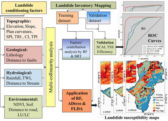
2.2. Methodology
2.3. LIM
2.4. Preparing Landslide Conditioning Factors (LCFs)
2.5. Testing Multi-Collinearity Problems
2.6. Landslide Susceptibility Modeling
2.6.1. Applying Random Forest (RF)
2.6.2. Applying Alternating Decision Tree (ADTree)
2.6.3. Applying Fisher’s Linear Discrimination Analysis (FLDA)
2.7. Considering the Contribution of Landslide Conditioning Factors
2.7.1. Boosted Regression Tree (BRT) Model
2.7.2. Application of Frequency Ratio Model
2.8. Methods for Validating the Models
3. Results
3.1. Considering Multi-Collinearity of Factors Contributing to Landslide Susceptibility
3.2. The Spatial Relationship Between Landslide Locations and Effective Factors by FR
3.3. Landslide Susceptibility Models
3.4. Validation of Machine Learning Models
4. Discussion
4.1. Model Performance and Comparison
4.2. Variable Contribution Analysis
5. Conclusions
Author Contributions
Funding
Acknowledgments
Conflicts of Interest
References
- Arabameri, A.; Pradhan, B.; Rezaei, K.; Sohrabi, M.; Kalantari, Z. GIS-based landslide susceptibility mapping using numerical risk factor bivariate model and its ensemble with linear multivariate regression and boosted regression tree algorithms. J. Mt. Sci. 2019, 16, 595–618. [Google Scholar] [CrossRef]
- IAEG Commission on Landslides. Suggested nomenclature for landslides. Bull. Int. Assoc. Eng. Geol. 1990, 41, 3–16. [Google Scholar] [CrossRef]
- Lin, L.; Lin, Q.; Wang, Y. Landslide susceptibility mapping on a global scale using the method of logistic regression. Nat. Hazards Earth Syst. Sci. 2017, 17, 1411–1424. [Google Scholar] [CrossRef] [Green Version]
- Nadim, F.; Kjekstad, O.; Peduzzi, P. Global landslide and avalanche hotspots. Landslides 2006, 3, 159–173. [Google Scholar] [CrossRef]
- Haftlang, K.K.; Lang, K.K.H. The Book of Iran: A Survey of the Geography of Iran; Alhoda: Tehran, UK, 2003; p. 17. ISBN 978-964-94491-3-5. [Google Scholar]
- Aghda, S.F.; Bagheri, V.; Razifard, M. Landslide Susceptibility Mapping Using Fuzzy Logic System and Its Influences on Mainlines in Lashgarak Region, Tehran, Iran. Geotech. Geol. Eng. 2018, 36, 915–937. [Google Scholar] [CrossRef]
- National Geosciences Database. 2017. Available online: www.ngdir.ir (accessed on 21 August 2018).
- Piacentini, D.; Devoto, S.; Mantovani, M.; Pasuto, A.; Prampolini, M.; Soldati, M. Landslide susceptibility modeling assisted by Persistent Scatterers Interferometry (PSI): An example from the northwestern coast of Malta. Nat. Hazards 2015, 78, 681–697. [Google Scholar] [CrossRef] [Green Version]
- Pradhan, A.M.S.; Kim, Y.T. Relative effect method of landslide susceptibility zonation in weathered granite soil: A case study in Deokjeok-ri Creek, South Korea. Nat. Hazards 2014, 72, 1189–1217. [Google Scholar] [CrossRef]
- Hong, H.; Tsangaratos, P.; Ilia, I. Application of fuzzy weight of evidence and data mining techniques in construction of flood susceptibility map of Poyang County, China. Sci. Total Environ. 2018, 625, 575–588. [Google Scholar] [CrossRef]
- Hong, H.; Liu, J.; Bui, D.T.; Pradhan, B.; Acharya, T.D.; Pham, B.T.; Ahmad, B.B. Landslide susceptibility mapping using J48 Decision Tree with AdaBoost, Bagging and Rotation Forest ensembles in the Guangchang area (China). Catena 2018, 163, 399–413. [Google Scholar] [CrossRef]
- Ahlmer, A.K.; Cavalli, M.; Hansson, K.; Koutsouris, A.J.; Crema, S.; Kalantari, Z. Soil moisture remote-sensing applications for identification of flood-prone areas along transport infrastructure. Environ. Earth Sci. 2018, 77, 533. [Google Scholar] [CrossRef] [Green Version]
- Nsengiyumva, J.; Luo, G.; Nahayo, L.; Huang, X.; Cai, P. Landslide Susceptibility Assessment Using Spatial Multi-Criteria Evaluation Model in Rwanda. Int. J. Environ. Res. Public Health 2018, 15, 243. [Google Scholar] [CrossRef] [Green Version]
- Chen, W.; Xie, X.; Peng, J.; Shahabi, H.; Hong, H.; Bui, D.T.; Duan, Z.; Li, S.; Zhu, A.X. GIS-based landslide susceptibility evaluation using a novel hybrid integration approach of bivariate statistical based random forest method. Catena 2018, 1–17. [Google Scholar] [CrossRef]
- Ayalew, L.; Yamagishi, H. The application of GIS-based logistic regression for landslide susceptibility mapping in the Kakuda-Yahiko Mountains, Central Japan. Geomorphology 2005, 65, 15–31. [Google Scholar] [CrossRef]
- Aleotti, P.; Chowdhury, R. Landslide hazard assessment: Summary review and new perspectives. Bull. Eng. Geol. Environ. 1999, 58, 21–44. [Google Scholar] [CrossRef]
- Arabameri, A.R.; Pourghasemi, H.R.; Yamani, M. Applying different scenarios for landslide spatial modeling using computational intelligence methods. Environ. Earth Sci. 2017, 76, 832. [Google Scholar] [CrossRef]
- Pradhan, B.; Jebur, M.N.; Shafri, H.Z.M.; Tehrany, M.S. Data fusion technique using wavelet transform and taguchi methods for automatic landslide detection from airborne laser scanning data and QuickBird satellite imagery. Trans. Geosci. Remote Sens. 2016, 54, 1–13. [Google Scholar] [CrossRef]
- Pham, B.T.; Bui, D.T.; Pourghasemi, H.R.; Indra, P.; Dholakia, M.B. Landslide susceptibility assessment in the Uttarakhand area (India) using GIS: A comparison study of prediction capability of naïve bayes, multilayer perceptron neural networks, and functional trees methods. Theor. Appl. Climatol. 2017, 128, 255–273. [Google Scholar] [CrossRef]
- Arabameri, A.; Pradhan, B.; Rezaei, K.; Lee, C.W. Assessment of Landslide Susceptibility Using Statistical-and Artificial Intelligence-Based FR–RF Integrated Model and Multiresolution DEMs. Remote Sens. 2019, 11, 999. [Google Scholar] [CrossRef] [Green Version]
- Arabameri, A.; Pradhan, B.; Pourghasemi, H.; Rezaei, K.; Kerle, N. Spatial Modelling of Gully Erosion Using GIS and R Programing: A Comparison among Three Data Mining Algorithms. Appl. Sci. 2018, 8, 1369. [Google Scholar] [CrossRef] [Green Version]
- Arabameri, A.; Rezaei, K.; Pourghasemi, H.R.; Lee, S.; Yamani, M. GIS based gully erosion susceptibility mapping: A comparison among three data-driven models and AHP knowledge-based technique. Environ. Earth Sci. 2018, 77, 628. [Google Scholar] [CrossRef]
- Arabameri, A.; Pradhan, B.; Rezaei, K.; Yamani, M.; Pourghasemi, H.R.; Lombardo, L. Spatial modelling of gully erosion using Evidential Belief Function, Logistic Regression and a new ensemble EBF–LR algorithm. Land Degrad. Dev. 2018, 29, 4035–4049. [Google Scholar] [CrossRef]
- Arabameri, A.; Pourghasemi, H.R. Spatial Modeling of Gully Erosion Using Linear and Quadratic Discriminant Analyses in GIS and R. In Spatial Modeling in GIS and R for Earth and Environmental Sciences, 1st ed.; Pourghasemi, H.R., Gokceoglu, C., Eds.; Elsevier: Amsterdam, The Netherlands, 2019. [Google Scholar]
- Arabameri, A.; Pradhan, B.; Rezaei, K. Gully erosion zonation mapping using integrated geographically weighted regression with certainty factor and random forest models in GIS. J. Environ. Manag. 2019, 232, 928–942. [Google Scholar] [CrossRef]
- Arabameri, A.; Rezaei, K.; Cerdà, A.; Conoscenti, C.; Kalantari, Z. A comparison of statistical methods and multi-criteria decision making to map flood hazard susceptibility in Northern Iran. Sci. Total Environ. 2019, 660, 443–458. [Google Scholar] [CrossRef]
- Arabameri, A.; Rezaei, K.; Cerda, A.; Lombardo, L.; Rodrigo-Comino, J. GIS-based groundwater potential mapping in Shahroud plain, Iran. A comparison among statistical (bivariate and multivariate), data mining and MCDM approaches. Sci. Total Environ. 2019, 658, 160–177. [Google Scholar] [CrossRef]
- Arabameri, A.; Pradhan, B.; Rezaei, K. Spatial prediction of gully erosion using ALOS PALSAR data and ensemble bivariate and data mining models. Geosci. J. 2019, 1, 1–18. [Google Scholar] [CrossRef]
- Chen, W.; Pourghasemi, H.R.; Zhao, Z. A GIS-based comparative study of Dempster-Shafer, logistic regression and artificial neural network models for landslide susceptibility mapping. Geocarto Int. 2017, 32, 367–385. [Google Scholar] [CrossRef]
- Hong, H.; Liu, J.; Zhu, A.X.; Shahabi, H.; Pham, B.T.; Chen, W.; Pradhan, B.; Bui, D.T. A novel hybrid integration model using support vector machines and random subspace for weather-triggered landslide susceptibility assessment in the Wuning area (China). Environ. Earth Sci. 2017, 76, 689. [Google Scholar] [CrossRef]
- Tien Bui, D.; Shahabi, H.; Shirzadi, A.; Chapi, K.; Pradhan, B.; Chen, W.; Khosravi, K.; Panahi, M.; Bin Ahmad, B.; Saro, L. Land subsidence susceptibility mapping in south korea using machine learning algorithms. Sensors 2018, 18, 2464. [Google Scholar] [CrossRef] [Green Version]
- Regmi, A.D.; Devkota, K.C.; Yoshida, K.; Pradhan, B.; Pourghasemi, H.R.; Kumamoto, T.; Akgun, A. Application of frequency ratio, statistical index, and weights-of-evidence models and their comparison in landslide susceptibility mapping in Central Nepal Himalaya. Arab. J. Geosci. 2014, 7, 725–742. [Google Scholar] [CrossRef]
- Roy, J.; Saha, S. Assessment of land suitability for the paddy cultivation using analytical hierarchical process (AHP): A study on Hinglo river basin, Eastern India. Model. Earth Syst. Environ. 2018, 4, 601–618. [Google Scholar] [CrossRef]
- Roy, J.; Saha, S. Landslide susceptibility mapping using knowledge driven statistical models in Darjeeling District, West Bengal, India. Geoenviron. Disasters 2019, 6, 11. [Google Scholar] [CrossRef] [Green Version]
- Roy, J.; Saha, S. GIS-based Gully Erosion Susceptibility Evaluation Using Frequency Ratio, Cosine Amplitude and Logistic Regression Ensembled with fuzzy logic in Hinglo River Basin, India. Remote Sens. Appl. Soc. Environ. 2019, 15, 100247. [Google Scholar] [CrossRef]
- Roy, J.; Saha, S.; Arabameri, A.; Blaschke, T.; Bui, D.T. A Novel Ensemble Approach for Landslide Susceptibility Mapping (LSM) in Darjeeling and Kalimpong Districts, West Bengal, India. Remote Sens. 2019, 11, 2866. [Google Scholar] [CrossRef] [Green Version]
- Saha, S. Groundwater potential mapping using analytical hierarchical process: A study on Md. Bazar Block of Birbhum District, West Bengal. Spat. Inf. Res. 2017, 25, 615–626. [Google Scholar] [CrossRef]
- Gayen, A.; Pourghasemi, H.R.; Saha, S.; Keesstra, S.; Bai, S. Gully erosion susceptibility assessment and management of hazard-prone areas in India using different machine learning algorithms. Sci. Total Environ. 2019, 668, 124–138. [Google Scholar] [CrossRef]
- Paul, G.C.; Saha, S.; Hembram, T.K. Application of the GIS-Based Probabilistic Models for Mapping the Flood Susceptibility in Bansloi Sub-basin of Ganga-Bhagirathi River and Their Comparison. Remote Sens. Earth Syst. Sci. 2019. [Google Scholar] [CrossRef]
- Lee, M.J.; Choi, J.W.; Oh, H.J.; Won, J.S.; Park, I.; Lee, S. Ensemble based landslide susceptibility maps in Jinbu area. Korea. Environ. Earth. Sci. 2012, 67, 23–37. [Google Scholar] [CrossRef]
- Arabameri, A. Application of the Analytic Hierarchy Process (AHP) for locating fire stations: Case study Maku City. Merit Res. J. Art Soc. Sci. Humanit. 2014, 2, 1–10. [Google Scholar]
- Arabameri, A.; Ramesht, M.H. Site Selection of Landfill with emphasis on Hydrogeomorphological–environmental parameters Shahrood-Bastam watershed. Sci. J. Manag. Syst. 2017, 16, 55–80. [Google Scholar]
- Arabameri, A. Zoning Mashhad Watershed for artificial recharge of underground aquifers using topsis model and GIS technique. Glob. J. Hum. Soc. Sci. B Geogr. Geo Sci. Environ. Disaster Manag. 2014, 14, 45–53. [Google Scholar]
- Arabameri, A.; Roy, J.; Saha, S.; Blaschke, T.; Ghorbanzadeh, O.; Tien Bui, D. Application of Probabilistic and Machine Learning Models for Groundwater Potentiality Mapping in Damghan Sedimentary Plain, Iran. Remote Sens. 2019, 11, 3015. [Google Scholar] [CrossRef] [Green Version]
- Tien Bui, D.; Le, K.T.; Nguyen, V.; Le, H.; Revhaug, I. Tropical forest fire susceptibility mapping at the Cat Ba National Park Area, Hai Phong City, Vietnam, using GIS-based Kernel logistic regression. Remote Sens. 2016, 8, 347. [Google Scholar] [CrossRef] [Green Version]
- Saadat, H.; Bonnell, R.; Sharifi, F.; Mehuys, G.; Namdar, M.; Ale-Ebrahim, S. Landform classification from a digital elevation model and satellite imagery. Geomorphology 2008, 100, 453–464. [Google Scholar] [CrossRef]
- Thai Pham, B.; Shirzadi, A.; Shahabi, H.; Omidvar, E.; Singh, S.K.; Sahana, M.; Talebpour Asl, D.; Bin Ahmad, B.; Kim Quoc, N.; Lee, S. Landslide Susceptibility Assessment by Novel Hybrid Machine Learning Algorithms. Sustainability 2019, 11, 4386. [Google Scholar] [CrossRef] [Green Version]
- Pham, B.T.; Prakash, I. Evaluation and comparison of LogitBoost Ensemble, Fisher’s Linear Discriminant Analysis, logistic regression and support vector machines methods for landslide susceptibility mapping. Geocarto Int. 2017, 3, 316–333. [Google Scholar] [CrossRef]
- Freund, Y.; Mason, L. The Alternating Decision Tree Learning Algorithm; ICML: New York, NY, USA, 1999; pp. 124–133. [Google Scholar]
- IRIMO. Summary Reports of Iran’s Extreme Climatic Events. Ministry of Roads and Urban Development, Iran Meteorological Organization. Available online: www.cri.ac.ir (accessed on 28 August 2018).
- Azari, M.; Saghafian, B.; Moradi, H.R.; Faramarzi, M. Effectiveness of Soil and Water Conservation Practices Under Climate Change in the Gorganroud Basin, Iran. Clean Soil Air Water 2017, 45, 1700288. [Google Scholar] [CrossRef]
- Shahpasandzadeh, M. Seismology and Seismotectonics of Golestan Province, Northeast Iran; International Institute Seismology and Earthquake Engineering, Seismology Research Institute of the Seismic Group: Tehran, Iran, 2004; p. 8. (In Persian) [Google Scholar]
- Lar Consulting Engineering. The Study on Flood and Debris Flow in the Golestan Province, Regional Water Board in Golestan; Ministry of Energy: Tehran, Iran, 2007. [Google Scholar]
- Jenks, G.F. The Data Model Concept in Statistical Mapping. Int. Yearb. Cartogr. 1967, 7, 186–190. [Google Scholar]
- McMaster, R. In Memoriam: George F. Jenks (1916–1996). Cartogr. Geogr. Inf. Sci. 1997, 24, 56–59. [Google Scholar] [CrossRef]
- Yilmaz, C.; Topal, T.; Suzen, M.L. GIS-based landslide susceptibility mapping using bivariate statistical analysis in Devrek (Zonguldak-Turkey). Environ. Earth Sci. 2012, 65, 2161–2178. [Google Scholar] [CrossRef]
- Van Westen, C.J.; van Asch, T.W.J.; Soeters, R. Landslide hazard and risk zonation—Why is it still so difficult? Bull. Eng. Geol. Environ. 2006, 65, 167–184. [Google Scholar] [CrossRef]
- Youssef, A.M.; Maerz, N.H.; Hassan, A.M. Remote sensing applications to geological problems in Egypt: Case study, slope instability investigation, Sharm El-Sheikh/Ras- Nasrani Area, Southern Sinai. Landslides 2009, 6, 353–360. [Google Scholar] [CrossRef]
- Iranian Landslide Working Party (ILWP). Iranian Landslides List; Forest, Rangeland and Watershed Association: Tehran, Iran, 2007; p. 60. [Google Scholar]
- Forestry, Rangeland and Watershed Organization (FRWO). List of Landslides in the Iran; Study Group on Landslides, Office of Engineering and Design Evaluation: 2013. Available online: http://www.frw.org.ir/02/Fa/default.aspx (accessed on 2 February 2020).
- Arabameri, A.; Pradhan, B.; Rezaei, K.; Lee, S.; Sohrabi, M. An ensemble model for landslide susceptibility mapping in a forested area. Geocarto Int. 2019. [Google Scholar] [CrossRef]
- Chung, C.-J.F.; Fabbri, A.G. Validation of spatial prediction models for landslide hazard mapping. Nat. Hazards 2003, 30, 451–472. [Google Scholar] [CrossRef]
- Marchesini, I.; Ardizzone, F.; Alvioli, M.; Rossi, M.; Guzzetti, F. Non-susceptible landslide areas in Italy and in the Mediterranean region. Nat. Hazards Earth Syst. Sci. 2014, 14, 2215–2231. [Google Scholar] [CrossRef] [Green Version]
- Frattini, P.; Crosta, G.; Carrara, A. Techniques for evaluating the performance of landslide susceptibility models. Eng. Geol. 2010, 111, 66–72. [Google Scholar] [CrossRef]
- Li, Z.; Zhu, Q.; Gold, C. Digital Terrain Modeling: Principles and Methodology; CRC Press: Boca Raton, FL, USA, 2005. [Google Scholar]
- Wentworth, C.K. A simplified method of determining the average slope of land surfaces. Am. J. Sci. 1930, 117, 184–194. [Google Scholar] [CrossRef]
- Zevenbergen, L.W.; Thorne, C.R. Quantitative analysis of land surface topography. Earth Surf. Process. Landf. 1987, 12, 47–56. [Google Scholar] [CrossRef]
- Moore, I.D.; Grayson, R.B.; Ladson, A.R. Digital terrain modelling: A review of hydrological, geomorphological, and biological applications. Hydrol. Process. 1991, 5, 3–30. [Google Scholar] [CrossRef]
- Gallant, J.C.; Wilson, J.P. Primary topographic attributes. In Terrain Analysis: Principles and Applications; Wilson, J.P., Gallant, J.C., Eds.; Wiley: New York, NY, USA, 2000; pp. 51–85. [Google Scholar]
- Wischmeier, W.H.; Smith, D.D. Predicting Rainfall Erosion Losses—A Guide to Conservation Planning; Agriculture Handbook No. 537; US Department of Agriculture Science and Education Administration: Washington, DC, USA, 1978; p. 163.
- Kiss, R. Determination of drainage network in digital elevation model. Util. Limit. J. Hung. Geomath. 2004, 2, 16–29. [Google Scholar]
- Ay, N.; Amari, S.-I. A Novel Approach to Canonical Divergences within Information Geometry. Entropy 2015, 17, 8111–8129. [Google Scholar] [CrossRef]
- Anderson, C.G.; Maxwell, D.C. Starting a Digitization Center; Elsevier: Amsterdam, The Netherlands, 2004; ISBN 978-1843340737. [Google Scholar]
- Bayraktar, H.; Turalioglu, S. A Kriging-based approach for locating a sampling site—In the assessment of air quality. Stoch. Environ. Res. Risk Assess. 2005, 19, 301–305. [Google Scholar] [CrossRef]
- Myung, I.J. Tutorial on Maximum Likelihood Estimation. J. Math. Psychol. 2003, 47, 90–100. [Google Scholar] [CrossRef]
- Crippen, R.E. Calculating the vegetation index faster. Remote Sens. Environ. 1990, 34, 71–73. [Google Scholar] [CrossRef]
- Pradhan, B.; Seeni, M.I.; Nampak, H. Integration of LiDAR and QuickBird data for automatic landslide detection using object-based analysis and random forests. In Laser Scanning Applications in Landslide Assessment; Pradhan, B., Ed.; Springer: Cham, Switzerland, 2017. [Google Scholar] [CrossRef]
- Cama, M.; Conoscenti, C.; Lombardo, L.; Rotigliano, E. Exploring relationships between grid cell size and accuracy for debris-flow susceptibility models: A test in the Giampilieri catchment (Sicily, Italy). Environ. Earth Sci. 2016, 75, 238. [Google Scholar] [CrossRef]
- Du, G.; Zhang, Y.; Iqbal, J. Landslide susceptibility mapping using an integrated model of information value method and logistic regression in the Bailongjiang watershed, Gansu Province, China. J. Mt. Sci. 2017, 14, 249. [Google Scholar] [CrossRef]
- Breiman, L. Random Forests. Mach. Learn. 2001, 45, 5–32. [Google Scholar] [CrossRef] [Green Version]
- Breiman, L.; Friedman, J.H.; Olshen, R.A.; Stone, C.J. Classification and Regression Trees; Chapman & Hall: New York, NY, USA, 1984. [Google Scholar]
- Hansen, L.; Salamon, P. Neural network ensembles. IEEE Trans. Pattern Anal. Mach. Intell. 1990, 12, 993–1001. [Google Scholar] [CrossRef] [Green Version]
- Breiman, L.; Cutler, A. Available online: http://www.stat.berkeley.edu/users/Breiman/RandomForests/ccpapers.html (accessed on 28 August 2018).
- Micheletti, N.; Foresti, L.; Robert, S.; Leuenberger, M.; Pedrazzini, A.; Jaboyedoff, M.; Kanevski, M. Machine learning feature selection methods for landslide susceptibility mapping. Math. Geosci. 2014, 46, 33–57. [Google Scholar] [CrossRef] [Green Version]
- Calle, M.L.; Urrea, V. Letter to the Editor: Stability of random forest importance measures. Brief. Bioinform. 2010, 12, 86–89. [Google Scholar] [CrossRef] [Green Version]
- Dietterich, T.G. An experimental comparison of three methods for constructing ensembles of decision trees: Bagging, boosting, and randomization. Mach. Learn. 2000, 40, 139–157. [Google Scholar] [CrossRef]
- Jolicoeur, P. Fisher_s linear discriminant function. In Introduction to Biometry; Springer: Berlin, Germany, 1999; pp. 303–308. [Google Scholar]
- Gilbert, E.S. The effect of unequal variance-covariance matrices on Fisher_s linear discriminant function. Biometrics 1969, 25, 505–515. [Google Scholar] [CrossRef]
- Yin, H.; Fu, P.; Meng, S. Sampled FLDA for face recognition with single training image per person. Neuro Comput. 2006, 69, 2443–2445. [Google Scholar] [CrossRef]
- Robinzonov, N. Advances in Boosting of Temporal and Spatial Models. Ludwig-Maximilians-Universitat München. 2013. Available online: http://edoc.ub.uni-muenchen.de/15338/ (accessed on 28 August 2018).
- Aertsen, W.; Kint, V.; Van Orshoven, J.; Muys, B. Evaluation of modelling techniques for forest site productivity prediction in contrasting ecoregions using stochastic multicriteria acceptability analysis (SMAA). Environ. Model. Softw. 2011, 26, 929–937. [Google Scholar] [CrossRef] [Green Version]
- James, G.; Witten, D.; Hastie, T. An Introduction to Statistical Learning; Springer: New York, NY, USA, 2013; pp. 856–875. [Google Scholar]
- Breiman, L. Arcing Classifiers. Ann. Stat. 1998, 26, 801–849. [Google Scholar] [CrossRef]
- Therneau, T.M.; Atkinson, B.; Ripley, B. RPART: Recursive Partitioning and Regression Trees. R Package Version 2014, 4, 1–8. [Google Scholar]
- Friedman, J.H. Greedy function approximation: A gradient boosting machine. Ann. Stat. 2001, 29, 1189–1232. [Google Scholar] [CrossRef]
- Williams, G.J. Data Mining with Rattle and R: The Art of Excavating Data for Knowledge Discovery; Springer: New York, NY, USA, 2011; p. 374. [Google Scholar] [CrossRef]
- Wang, Q.; Li, W. A GIS-based comparative evaluation of analytical hierarchy process and frequency ratio models for landslide susceptibility mapping. Phys. Geogr. 2017, 38, 318–337. [Google Scholar] [CrossRef]
- Rahmati, O.; Haghizadeh, A.; Pourghasemi, H.R.; Noormohamadi, F. Gully erosion susceptibility mapping: The role of GIS based bivariate statistical models and their comparison. Nat. Hazards 2016, 82, 1231–1258. [Google Scholar] [CrossRef]
- Oh, H.; Lee, S.; Hong, S.M. Landslide susceptibility assessment using frequency ratio technique with iterative random sampling. J. Sens. 2017, 1–21. [Google Scholar] [CrossRef] [Green Version]
- Pradhan, B. An Assessment of the use of an advanced neural network model with Five different training strategies for the preparation of landslide susceptibility maps. J. Data Sci. 2011, 9, 65–81. [Google Scholar]
- Arabameri, A.; Cerda, A.; Rodrigo-Comino, J.; Pradhan, B.; Sohrabi, M.; Blaschke, T.; Tien Bui, D. Proposing a Novel Predictive Technique for Gully Erosion Susceptibility Mapping in Arid and Semi-arid Regions (Iran). Remote Sens. 2019, 11, 2577. [Google Scholar] [CrossRef] [Green Version]
- Arabameri, A.; Chen, W.; Lombardo, L.; Blaschke, T.; Tien Bui, D. Hybrid Computational Intelligence Models for Improvement Gully Erosion Assessment. Remote Sens. 2020, 12, 140. [Google Scholar] [CrossRef] [Green Version]
- Arabameri, A.; Chen, W.; Loche, M.; Zhao, X.; Li, Y.; Lombardo, L.; Cerda, A.; Pradhan, B.; Bui, D.T. Comparison of machine learning models for gully erosion susceptibility mapping. Geosci. Front. 2019, in press. [Google Scholar] [CrossRef]
- Arabameri, A.; Cerda, A.; Tiefenbacher, J.P. Spatial pattern analysis and prediction of gully erosion using novel hybrid model of entropy-weight of evidence. Water 2019, 11, 1129. [Google Scholar] [CrossRef] [Green Version]
- Arabameri, A.; Chen, W.; Blaschke, T.; Tiefenbacher, J.P.; Pradhan, B.; Tien Bui, D. Gully Head-Cut Distribution Modeling Using Machine Learning Methods—A Case Study of N.W. Iran. Water 2020, 12, 16. [Google Scholar] [CrossRef] [Green Version]
- Arabameri, A.; Blaschke, T.; Pradhan, B.; Pourghasemi, H.R.; Tiefenbacher, J.P.; Bui, D.T. Evaluation of Recent Advanced Soft Computing Techniques for Gully Erosion Susceptibility Mapping: A Comparative Study. Sensors 2020, 20, 335. [Google Scholar] [CrossRef] [Green Version]
- Yesilnacar, E.; Topal, T. Landslide susceptibility mapping: A comparison of logistic regression and neural networks methods in a medium scale study, Hendek region (Turkey). Eng. Geol. 2005, 79, 251–266. [Google Scholar] [CrossRef]
- Oh, H.J.; Kim, Y.S.; Choi, J.K.; Park, E.; Lee, S. GIS mapping of regional probabilistic groundwater potential in the area of Pohang City. Korea. J. Hydrol. 2011, 399, 158–172. [Google Scholar] [CrossRef]
- Bui, D.T.; Pradhan, B.; Lofman, O.; Revhaug, I. Landslide susceptibility assessment in Vietnam using support vector machines, decision tree and Naïve Bayes models. Math. Probl. Eng. 2012, 2012, 974638. [Google Scholar]
- Oh, H.J.; Lee, S. Assessment of ground subsidence using GIS and the weights-of evidence model. Eng. Geol. 2010, 115, 36–48. [Google Scholar] [CrossRef]
- Corsini, A.; Cervi, F.; Ronchetti, F. Weight of evidence and artificial neural networks for potential groundwater spring mapping: An application to the Mt. Modino area (Northern Apennines, Italy). Geomorphology 2009, 111, 79–87. [Google Scholar] [CrossRef]
- Süzen, M.L.; Doyuran, V. A comparison of the GIS based landslide susceptibility assessment methods: Multivariate versus bivariate. Environ. Geol. 2004, 45, 665–679. [Google Scholar] [CrossRef]
- Allouche, O.; Tsoar, A.; Kadmon, R. Assessing the accuracy of species distribution models: Prevalence, kappa and the true skill statistic (TSS). J. Appl. Ecol. 2006, 43, 1223–1232. [Google Scholar] [CrossRef]
- Pradhan, B.; Hagemann, U.; Tehrany, M. An easy to use ArcMap based texture analysis program for extraction of flooded areas from TerraSAR-X satellite image. Comput. Geosci. 2013, 63, 34–43. [Google Scholar] [CrossRef]
- García-Davalillo, J.C.; Herrera, G.; Notti, D.; Strozzi, T.; Álvarez-Fernández, I. DInSAR analysis of ALOS PALSAR images for the assessment of very slow landslides: The Tena Valley case study. Landslides 2014, 11, 225–246. [Google Scholar] [CrossRef]
- Honda, K.; Nakanishi, T.; Haraguchi, M.; Mushiake, N.; Iwasaki, T.; Satoh, H.; Kobori, T.; Yamaguchi, Y. Application of Exterior Deformation Monitoring of Dams by DInSAR Analysis Using ALOS PALSAR; The IEEE International Geoscience and Remote Sensing Symposium (IGARSS): Munich, Germany, 2012. [Google Scholar]
- Blaschke, T. Object based image analysis for remote sensing. ISPRS J. Photogramm. Remote Sens. 2010, 65, 2–16. [Google Scholar] [CrossRef] [Green Version]


| Factors | Class | Data Used/Resolution/Scales | Data Sources | Techniques | Classification Methods | Ref. |
|---|---|---|---|---|---|---|
| Elevation (m) | 1. <354, 2. 354–768, 3. 768–1216, 4. 1216–658, 5. >1658 | ALOS DEM (12.5 m × 12.5 m resolution) | https//vertex.daac.asf.alaska.edu (Alaska Satellite Facility) | 12.5 m × 12.5 m DEM | Natural break (Jenks) | [65] |
| Slope (0) | 1. <5, 2. 5–10, 3. 10–15, 4. 20–30, 5. >30 | ALOS DEM (12.5 m × 15.5 m resolution) | https//vertex.daac.asf.alaska.edu (Alaska Satellite Facility) | where N = No. of Contour Cuttings; I = Contour Interval (12.5 m × 15.5 m resolution) | Natural break (Jenks) | [66] |
| PC | 1. Concave, 2. Flat, 3. Convex | ALOS DEM (12.5 m × 12.5 m resolution) | https//vertex.daac.asf.alaska.edu (Alaska Satellite Facility) | 12.5 m × 12.5 m DEM | Natural break (Jenks) | [67] |
| SPI | 1. <9.08, 2. 9.08–10.99, 3. 10.99–12.9, 4. 12.9–15.8, 5. >15.8 | ALOS DEM (12.5 m × 12.5 m resolution) | https//vertex.daac.asf.alaska.edu (Alaska Satellite Facility) | where AS is the upstream contributing area and β is the slope gradient (in degrees) | Natural break (Jenks) | [68] |
| TPI | 1. <−1.83, 2. −1.83–−0.18, 3. −0.18–1.37, 4. 1.37–3.99, 5. >3.99 | ALOS DEM (12.5 m × 12.5 m resolution) | https//vertex.daac.asf.alaska.edu (Alaska Satellite Facility) | Center point elevation (Z0) and the average elevation () around it within a predetermined radius (R) | Natural break (Jenks) | [69] |
| TWI | 1. <4.89, 2. 4.89–7.33, 3. 7.33–11.08, 4. >11.08 | ALOS DEM (12.5 m × 12.5 m resolution) | https//vertex.daac.asf.alaska.edu (Alaska Satellite Facility) | where α not in formula is a total upsloped area that drains through a point (per unit contour length), β not in formula is a gradient of the slope (in degree). | Natural break (Jenks) | [68] |
| LS (m) | 1. <30.7, 2. 30.7–65.08, 3. 65.08–101.1, 4. 101.1–140.7, 5. >140.7 | ALOS DEM (12.5 m × 12.5 m resolution) | https//vertex.daac.asf.alaska.edu (Alaska Satellite Facility) | where AS is the particular area of the basin (m2 m−1) and β is the slope in degrees. | Natural break (Jenks) | [70] |
| CI (100/M) | 1. <−32.54, 2. −32.54–-9.8, 3. −9.8–9.01, 4. 9.01–31.76, 5. >31.76 | ALOS DEM (12.5 m × 12.5 m resolution) | https//vertex.daac.asf.alaska.edu (Alaska Satellite Facility) | where θ indicates the average angle between the aspect of adjacent cells and the direction to the central cell. | Natural break (Jenks) | [71] |
| Dis to fault (m) | 1. <500, 2. 500–1000, 3. 1000–1500, 4. 1500–2000, 5. >2000 | ETM+2002 satellite data (15 m × 15 m) | Soil Conservation Section of the Agricultural and Natural Resources Research Center | Euclidian Distance Buffering | Natural break (Jenks) | [72] |
| Dis to road (m) | 1. <500, 2. 500–1000, 3. 1000–1500, 4. 1500–2000, 5. >2000 | Topographical map (scale 1: 25,000) and Google Earth image | Cartography department of Iran | Digitization process | Natural break (Jenks) | [73] |
| Dis to stream (m) | 1. <100, 2. 100–200, 3. 200–300, 4. 300–400, 5. >400 | ALOS DEM (12.5 m × 12.5 m resolution) | https//vertex.daac.asf.alaska.edu (Alaska Satellite Facility) | Euclidian Distance Buffering | Natural break (Jenks) | [72] |
| Rainfall (mm) | 1. <425.9, 2. 425.9–561.6, 3. 561.6–703.6, 4. 703.6–851.9, 5. >851.9 | 30 years average rainfall data of different stations | Islamic Republic of Iran metrological Organization | Kriging Interpolation method | Natural break (Jenks) | [74] |
| Lithology | 1. A, 2. B, 3. C, 4. D, 5. E, 6. F, 7.G, 8. H | Projected geological map (scale 1:100,000) | Geological survey of Iran | Digitization process | Equal interval | [73] |
| LU/LC | 1. Afforest, 2. Agriculture, 3. Orchard, 4. Dry farming, 5. Water, 6. Agri-Orch, 7. Rock, 8. Urban | Landsat 8 OLI/TIRS (Path 162/Row 34) (30 m × 30 m resolution) | U.S Geological Survey | Supervised classification (Maximum likelihood) | Maximum likelihood | [75] |
| NDVI | 1. <−0.201, 2. −0.201–0.36, 3. >0.36 | Landsat 8 OLI/TIRS (Path 162/Row 34) (30 m × 30 m resolution) | U.S Geological Survey | where NIR is near inferred band or band 4 and IR is the infrared band or band 3. | Natural break (Jenks) | [76] |
| Soil type | 1. Rock Outcrops/Entisols, 2. Inceptisols, 3. Mollisols, 4. Alfisols | Projected soil map (Scale 1:25,000) | Agricultural and Natural Resources Research Center in Iran | Digitization process | Equal interval | [73] |
| Unstandardized Coefficients | Standardized Coefficients | t | Sig. | Collinearity Statistics | |||
|---|---|---|---|---|---|---|---|
| B | Std. Error | Beta | Tolerance | VIF | |||
| (Constant) | −1.017 | 0.222 | − | −4.580 | 0.000 | − | − |
| Rainfall | 0.001 | 0.000 | 0.269 | 3.644 | 0.000 | 0.392 | 2.552 |
| Soil type | 0.303 | 0.111 | 0.150 | 2.744 | 0.006 | 0.711 | 1.407 |
| LU/LC | 0.186 | 0.040 | 0.249 | 4.710 | 0.000 | 0.766 | 1.306 |
| Lithology | 0.223 | 0.063 | 0.174 | 3.547 | 0.000 | 0.883 | 1.132 |
| Slope | −0.005 | 0.004 | −0.094 | −1.162 | 0.246 | 0.324 | 3.085 |
| Dis to road | −2.427 × 10⁻⁵ | 0.000 | −0.111 | −2.177 | 0.030 | 0.824 | 1.214 |
| TWI | −0.060 | 0.019 | −0.402 | −3.162 | 0.002 | 0.232 | 4.566 |
| Dis to fault | −1.372 × 10⁻⁵ | 0.000 | −0.090 | −1.594 | 0.112 | 0.667 | 1.498 |
| PC | 0.008 | 0.008 | 0.053 | 1.028 | 0.305 | 0.800 | 1.249 |
| TPI | 0.011 | 0.006 | 0.082 | 1.723 | 0.086 | 0.955 | 1.048 |
| Elevation | 0.000 | 0.000 | −0.146 | −2.512 | 0.012 | 0.628 | 1.592 |
| NDVI | −0.453 | 0.268 | −0.122 | −1.692 | 0.092 | 0.410 | 2.437 |
| CI | 0.000 | 0.001 | 0.021 | .351 | 0.726 | 0.593 | 1.687 |
| Dis to stram | 0.000 | 0.000 | −0.141 | −2.705 | 0.007 | 0.785 | 1.274 |
| SPI | 0.092 | 0.021 | 0.506 | 4.337 | 0.000 | 0.257 | 4.368 |
| LS | −0.056 | 0.014 | −0.345 | −3.167 | 0.004 | 0.332 | 2.756 |
| Factors | Class | Pixels in Domain | Pixels of Landslide | FR | ||
|---|---|---|---|---|---|---|
| No | % | No | % | |||
| Elevation (m) | <354 | 1,757,987 | 28.85 | 64 | 39.02 | 1.35 |
| 354–768 | 1,528,329 | 25.08 | 48 | 29.27 | 1.17 | |
| 768–1216 | 1,255,594 | 20.60 | 40 | 24.39 | 1.18 | |
| 1216–1658 | 979,570 | 16.07 | 11 | 6.71 | 0.42 | |
| >1658 | 573,032 | 9.40 | 1 | 0.61 | 0.06 | |
| Slope (0) | <5 | 1,533,843 | 25.17 | 33 | 20.12 | 0.80 |
| 5–10 | 877,089 | 14.39 | 42 | 25.61 | 1.78 | |
| 10–15 | 1,031,179 | 16.92 | 27 | 16.46 | 0.97 | |
| 15–20 | 947,857 | 15.56 | 17 | 10.37 | 0.67 | |
| 20–30 | 1,198,335 | 19.67 | 37 | 22.56 | 1.15 | |
| >30 | 505,070 | 8.29 | 8 | 4.88 | 0.59 | |
| PC | Concave | 2,686,090 | 44.08 | 79 | 48.17 | 1.09 |
| Flat | 528,638 | 8.68 | 6 | 3.66 | 0.42 | |
| Convex | 2,878,644 | 47.24 | 79 | 48.17 | 1.02 | |
| SPI | <9.08 | 893,698 | 14.68 | 11 | 6.71 | 0.46 |
| 9.08–10.99 | 2,044,913 | 33.60 | 61 | 37.20 | 1.11 | |
| 10.99–12.9 | 2,162,864 | 35.54 | 58 | 35.37 | 1.00 | |
| 12.9–15.8 | 801,588 | 13.17 | 18 | 10.98 | 0.83 | |
| >15.8 | 182,979 | 3.01 | 16 | 9.76 | 3.24 | |
| TPI | <−1.83 | 303,487 | 4.98 | 8 | 4.88 | 0.98 |
| −1.83–−0.18 | 1,031,274 | 16.92 | 23 | 14.02 | 0.83 | |
| −0.18–1.37 | 1,212,301 | 19.89 | 26 | 15.85 | 0.80 | |
| 1.37–3.99 | 492,748 | 8.09 | 17 | 10.37 | 1.28 | |
| >3.99 | 3,054,702 | 50.12 | 90 | 54.88 | 1.09 | |
| TWI | <4.89 | 2,838,332 | 46.57 | 73 | 44.51 | 0.96 |
| 4.89–7.33 | 2,261,932 | 37.11 | 60 | 36.59 | 0.99 | |
| 7.33–11.08 | 798,883 | 13.11 | 14 | 8.54 | 0.65 | |
| >11.08 | 195,364 | 3.21 | 17 | 10.37 | 3.23 | |
| LS (m) | <30.7 | 781,241 | 25.68 | 19 | 22.62 | 0.88 |
| 30.7–65.08 | 720,877 | 23.69 | 20 | 23.81 | 1.00 | |
| 65.08–101.1 | 632,770 | 20.80 | 30 | 35.71 | 1.72 | |
| 101.1–140.7 | 527,320 | 17.33 | 10 | 11.90 | 0.69 | |
| >140.7 | 380,217 | 12.50 | 5 | 5.95 | 0.48 | |
| CI (100/M) | <−32.54 | 586,802 | 9.63 | 22 | 13.41 | 1.39 |
| −32.54–−9.8 | 1,196,806 | 19.64 | 37 | 22.56 | 1.15 | |
| −9.8–9.01 | 2,386,816 | 39.17 | 64 | 39.02 | 1.00 | |
| 9.01–31.76 | 1,387,504 | 22.77 | 31 | 18.90 | 0.83 | |
| >31.76 | 536,304 | 8.80 | 10 | 6.10 | 0.69 | |
| Dis to road (m) | <500 | 762,121 | 12.51 | 46 | 28.05 | 2.24 |
| 500–1000 | 709,095 | 11.64 | 30 | 18.29 | 1.57 | |
| 1000–1500 | 652,772 | 10.71 | 14 | 8.54 | 0.80 | |
| 1500–2000 | 591,152 | 9.70 | 7 | 4.27 | 0.44 | |
| >2000 | 3,378,964 | 55.45 | 67 | 40.85 | 0.74 | |
| Dis to stream (m) | <100 | 1,058,295 | 17.38 | 70 | 42.68 | 2.46 |
| 100–200 | 844,165 | 13.86 | 29 | 17.68 | 1.28 | |
| 200–300 | 834,301 | 13.70 | 10 | 6.10 | 0.45 | |
| 300–400 | 644,273 | 10.58 | 9 | 5.49 | 0.52 | |
| >400 | 2,708,520 | 44.48 | 46 | 28.05 | 0.63 | |
| Rainfall (mm) | <425.9 | 929,156 | 15.25 | 2 | 1.22 | 0.08 |
| 425.9–561.6 | 1,861,610 | 30.56 | 86 | 52.44 | 1.72 | |
| 561.6–703.6 | 1,490,446 | 24.47 | 18 | 10.98 | 0.45 | |
| 703.6–851.9 | 1,176,590 | 19.31 | 25 | 15.24 | 0.79 | |
| >851.9 | 634,325 | 10.41 | 33 | 20.12 | 1.93 | |
| Lithology | A | 453,438 | 7.42 | 1 | 0.61 | 0.08 |
| B | 3,068,975 | 50.19 | 104 | 63.41 | 1.26 | |
| C | 74,810 | 1.22 | 0 | 0.00 | 0.00 | |
| D | 1,250,277 | 20.45 | 26 | 15.85 | 0.78 | |
| E | 543,327 | 8.89 | 13 | 7.93 | 0.89 | |
| F | 429,394 | 7.02 | 9 | 5.49 | 0.78 | |
| G | 236,729 | 3.87 | 6 | 3.66 | 0.95 | |
| H | 58,043 | 0.95 | 5 | 3.05 | 3.21 | |
| LU/LC | Afforest | 1,582,944 | 25.89 | 20 | 12.20 | 0.47 |
| Agriculture | 638,404 | 10.44 | 14 | 8.54 | 0.82 | |
| Orchard | 931 | 0.02 | 0 | 0.00 | 0.00 | |
| Dry farming | 2,883,017 | 47.15 | 74 | 45.12 | 0.96 | |
| Water | 42,648 | 0.70 | 1 | 0.61 | 0 | |
| Agri-Orch | 901,557 | 14.74 | 51 | 31.10 | 2.11 | |
| Rock | 5,361 | 0.09 | 1 | 0.61 | 6.95 | |
| Urban | 59,975 | 0.98 | 3 | 1.83 | 1.87 | |
| NDVI | <−0.201 | 3,517,295 | 57.72 | 98 | 59.76 | 1.04 |
| −0.201–0.36 | 929,798 | 15.26 | 41 | 25.00 | 1.64 | |
| >0.36 | 1,647,011 | 27.03 | 25 | 15.24 | 0.56 | |
| Soil type | Rock Outcrops/Entisols | 1,566,585 | 25.62 | 28 | 17.07 | 0.67 |
| Inceptisols | 1,210,719 | 19.80 | 36 | 21.95 | 1.11 | |
| Mollisols | 1,797,624 | 29.40 | 44 | 26.83 | 0.91 | |
| Alfisols | 1,540,065 | 25.19 | 56 | 34.15 | 1.36 | |
| Dis to fault (m) | <500 | 670,236 | 11.00 | 15 | 9.15 | 0.83 |
| 500–1000 | 637,781 | 10.47 | 14 | 8.54 | 0.82 | |
| 1000–1500 | 581,006 | 9.53 | 11 | 6.71 | 0.70 | |
| 1500–2000 | 503,170 | 8.26 | 11 | 6.71 | 0.81 | |
| >2000 | 3,701,746 | 60.74 | 113 | 68.90 | 1.13 | |
| Model | Class | Pixels in Domain | Pixels of Landslide | SCAI | ||
|---|---|---|---|---|---|---|
| No | % | No | % | |||
| ADTree | Very Low | 1,865,100 | 31.27 | 7 | 3.07 | 10.18 |
| Low | 2,255,466 | 37.81 | 43 | 18.86 | 2.00 | |
| Moderate | 91,472 | 1.53 | 5 | 2.19 | 0.70 | |
| High | 836,774 | 14.03 | 49 | 21.49 | 0.65 | |
| Very High | 916,639 | 15.37 | 124 | 54.39 | 0.28 | |
| FLDA | Very Low | 648,691 | 10.64 | 2 | 0.88 | 12.14 |
| Low | 1,352,591 | 22.20 | 7 | 3.07 | 7.23 | |
| Moderate | 1,522,829 | 24.99 | 30 | 13.16 | 1.90 | |
| High | 1,588,744 | 26.07 | 82 | 35.96 | 0.72 | |
| Very High | 981,082 | 16.10 | 107 | 46.93 | 0.34 | |
| RF | Very Low | 1,569,307 | 25.75 | 3 | 1.32 | 19.57 |
| Low | 1,743,560 | 28.61 | 3 | 1.32 | 21.75 | |
| Moderate | 1,185,580 | 19.46 | 14 | 6.14 | 3.17 | |
| High | 902,913 | 14.82 | 27 | 11.84 | 1.25 | |
| Very High | 692,408 | 11.36 | 181 | 79.39 | 0.14 | |
| Models | Validation Dataset (VD) | Training Dataset (TD) | ||||
|---|---|---|---|---|---|---|
| FLDA | RF | ADTree | FLDA | RF | ADTree | |
| TN | 44 | 58 | 54 | 122 | 128 | 117 |
| FP | 31 | 17 | 21 | 52 | 46 | 57 |
| FN | 16 | 17 | 25 | 40 | 35 | 51 |
| TP | 59 | 58 | 50 | 134 | 139 | 123 |
| TPR | 0.79 | 0.77 | 0.67 | 0.77 | 0.80 | 0.71 |
| FPR | 0.41 | 0.23 | 0.28 | 0.30 | 0.26 | 0.33 |
| efficiency | 0.69 | 0.77 | 0.69 | 0.74 | 0.77 | 0.69 |
| TSS | 0.37 | 0.55 | 0.39 | 0.47 | 0.53 | 0.38 |
| 0 | 1 | Class Error | |
|---|---|---|---|
| 0 | 113 | 6 | 0.0504 |
| 1 | 20 | 104 | 0.1612 |
| Factor | Weight |
|---|---|
| TPI | 21.09 |
| Distance to stream | 7.72 |
| Elevation | 5.8 |
| Rainfall | 8.17 |
| Plan curvature | 2.99 |
| Lithology | 2.78 |
| SPI | 4.42 |
| CI | 2.93 |
| TWI | 3.01 |
| Distance to road | 4.62 |
| NDVI | 3.31 |
| Soil | 1.42 |
| Distance to fault | 3.88 |
| Slope | 3.35 |
| LULC | 1.28 |
| LS | 1.01 |
© 2020 by the authors. Licensee MDPI, Basel, Switzerland. This article is an open access article distributed under the terms and conditions of the Creative Commons Attribution (CC BY) license (http://creativecommons.org/licenses/by/4.0/).
Share and Cite
Arabameri, A.; Saha, S.; Roy, J.; Chen, W.; Blaschke, T.; Tien Bui, D. Landslide Susceptibility Evaluation and Management Using Different Machine Learning Methods in The Gallicash River Watershed, Iran. Remote Sens. 2020, 12, 475. https://doi.org/10.3390/rs12030475
Arabameri A, Saha S, Roy J, Chen W, Blaschke T, Tien Bui D. Landslide Susceptibility Evaluation and Management Using Different Machine Learning Methods in The Gallicash River Watershed, Iran. Remote Sensing. 2020; 12(3):475. https://doi.org/10.3390/rs12030475
Chicago/Turabian StyleArabameri, Alireza, Sunil Saha, Jagabandhu Roy, Wei Chen, Thomas Blaschke, and Dieu Tien Bui. 2020. "Landslide Susceptibility Evaluation and Management Using Different Machine Learning Methods in The Gallicash River Watershed, Iran" Remote Sensing 12, no. 3: 475. https://doi.org/10.3390/rs12030475