Article

Remote Sensing and Social Sensing Data Reveal Scale-Dependent and System-Specific Strengths of Urban Heat Island Determinants

1
School of Life Sciences, Nanjing University, Nanjing 210023, China
2
Department of Geosciences and Natural Resource Management, Faculty of Science, University of Copenhagen, Copenhagen 1958, Denmark
3
School of Architecture and Urban Planning, Nanjing University, Nanjing 210093, China
4
Jiangsu Institute of Urban Planning and Design, Nanjing 210036, China
5
College of Life Sciences, Nanjing Normal University, Nanjing 210023, China
*
Author to whom correspondence should be addressed.
These authors contributed equally to this work.
Remote Sens. 2020, 12(3), 391; https://doi.org/10.3390/rs12030391
Submission received: 31 December 2019 / Revised: 17 January 2020 / Accepted: 20 January 2020 / Published: 26 January 2020

Abstract

:
Urban natural surfaces and non-surface human activities are key factors determining the urban heat island (UHI), but their relative importance remains highly controversial and may vary at different spatial scales and focal urban systems. However, systematic studies on the scale-dependency system-specificity remain largely lacking. Here, we selected 32 major Chinese cities as cases and used Landsat 8 images to retrieve land surface temperature (LST) and quantify natural surface variables using point of interest (POI) data as a measure of the human activity variable and using multiple regression and relative weight analysis to study the contribution and relative importance of these factors to LST at a range of grain sizes (0.25–5 km) and spatial extents (20–60 km). We revealed that the contributions and relative importance of natural surfaces and human activities are largely scale-dependent and system-specific. Natural surfaces, especially vegetation cover, are often the most important UHI determinants for a majority of scales, but the importance of non-surface human activities is increasingly pronounced at a coarser spatial scale with respect to both grain and spatial extent. The scaling relations of the UHI determinants and their relative importance were mostly linear-like at the city-collective level, but highly diverse across individual cities, so reducing non-surface heat emissions could be the most effective measure in particular cases, especially at relatively large spatial scales. This study advances the understanding of UHI formation mechanisms and highlights the complexity of the scale issue underpinning the UHI effect.

Graphical Abstract

1. Introduction

According to the projection of the United Nations, urban residents will account for 70% of the world’s total population by the middle of this century [1]. Urbanization has profoundly transformed the Earth’s land surfaces and modified the composition, structure, and energy flow of the atmospheric system in the near-surface layer [2,3]. Among these remarkable urbanization-induced modifications is the urban heat island (UHI) effect, referred to as the phenomenon of urban temperatures being higher than those in rural surroundings [4,5,6,7,8]. Studies on the UHI effect are gaining momentum across a wide range of research fields, with particular concerns given to its negative environmental and social impacts such as deteriorated air quality [9], excessive consumption of water and power [2], and impaired human health [10]. Therefore, there is an urgent need for us to take measures to help mitigate the UHI effect. Furthermore, a comprehensive, quantitative understanding of the determinants of UHIs would help to choose the most efficient mitigating measures.
Typically, the UHI effect can be quantified based on the measurement of near-surface air temperature (referred to as atmospheric UHIs) or land surface temperature (referred to as surface UHIs) [11,12]. Facilitated by readily available remotely sensed data, recent studies have increasingly focused on land surface temperature (LST) as a direct indicator of the surface UHI effect to study how UHIs are shaped by an array of environmental and anthropogenic determinants [13,14,15,16]. It has been well documented that remotely sensed LST is strongly correlated with natural-surface biophysical variables that characterize vegetation and water cover, suggesting that urban vegetation and water bodies have a significant cooling effect [4,14,17,18]. A set of remotely sensed indicators of natural-surface properties such as the normalized difference vegetation index (NDVI), the leaf area index (LAI), and the normalized difference water index (NDWI) has therefore been adopted in studies aimed at unraveling the driving factors of UHIs [19,20].
However, these natural-surface factors are not the only determinants of UHIs [6] because some human activities that do not modify the physical properties of land surfaces can also contribute to UHI formation. For example, two separate land units that accommodate substantially different resident densities, with all else being equal, would emit different amounts of heat (for the purpose of e.g., stabilizing indoor environments), thus resulting in differential local thermal environments. Indeed, a handful of empirical studies has suggested that population density and societal status (in terms of income and education level) have significant effects driving the formation of UHIs [7,10,21].
One barrier for us in the study of the human influence of LST is that the quick development of remote sensing technology allows us to extract high-resolution LST and natural-surface data, while the social sensing data are usually restricted by the administrative census. Fortunately, the rapid development of Internet technology and the increasing availability of open big data are substantially alleviating this difficulty. In recent years, the development of social sensing technology has produced a rich set of high-resolution data, allowing for the quantitative characterization of human activities in detail [22,23]. Many social sensing data (such as social media data, public transport data, and location-based service data) have been mined, giving rise to a range of interesting socioeconomic structures and dynamics that have been previously impossible to reveal [22,24]. One particular useful source is the Point of Interest (POI) data, which provides location-based geographic information and other detailed information for each geographic element on the map [25]. POI contains almost all types of human activities in the city, and are suggested to be able to well reflect the intensity of human activities and anthropogenic heat emissions [22,25,26]. While increasing attention is being paid to these non-surface factors, their strengths relative to the land-surface factors remain unclear.
Assessing the relative importance of the surface vs. non-surface factors in shaping the UHI effect (hereafter referred to as the relative importance problem, RIP) is highly relevant to the mechanistic understanding of the UHI effect. It also has important implications for the decision making of urban climate mitigation [27,28]. For example, at specific conditions, if a UHI pattern is predominantly determined by the natural surface properties, the effectiveness of measures for cooling down the urban environment would largely rely on the design of the urban green system. However, the answer to the RIP remains elusive, as contrasting conclusions have been reached in previous studies. On one hand, it has been suggested that compared with human activities, the biophysical properties of land (especially natural) surfaces can largely determine the latent and sensible heat flux and generally contribute the most to LST pattern and intensity [2,3,29]. On the other hand, it has been stressed that non-surface human activities also play a key role in shaping UHIs through contributing an important, direct heat source, particularly in high-density neighborhoods at local spatial scales [5,6,8,30].
This active debate on the RIP of UHI determinants may be undermined by some important confounding factors that have not been explicitly addressed. First, it remains poorly understood if and to what extent the RIP answer is specific or universal to different urban systems. Regarding previous studies that have largely been based on single urban systems, a more comprehensive understanding would necessarily invoke systematic investigations that take into account multiple urban systems across a wide geographic range. Second, it remains unclear if and how the RIP answer is dependent on the observational scale. Previous work has shown that the spatial pattern of LST, as well as its driving factors, are sensitive to the spatial resolution of the remotely sensed data used [15,21,27,28,31], implying that the RIP solution is plausibly dependent on grain size (as a fundamental dimension of spatial scale). A complete understanding of the role of scale requires systematic scaling analyses that consider both the spatial extent and grain size.
Therefore, in this study, to clearly answer these insufficiencies, we assessed the relative strengths of natural-surface vs. non-surface factors in shaping the LST patterns across 32 major Chinese cities. We focused on the natural surfaces (including vegetation and water) because they have been recognized as essential “ecological infrastructure” for mitigating the UHI effect. We used the Landsat-8 OLI remote sensing data and the POI social sensing data to characterize natural-surface properties and non-surface human activities, respectively. We then assessed their relative importance in explaining the observed LST patterns across a range of spatial scales in terms of grain size and spatial extent. We aimed to answer two specific questions: (1) Is the relative importance between natural-surface vs. non-surface factors dependent on observational scales? and (2) Is the relative importance specific to different urban systems? Finally, we hope that this study will provide implications for understanding the mechanism of UHI formation and UHI mitigation practices.

2. Materials and Data Processing

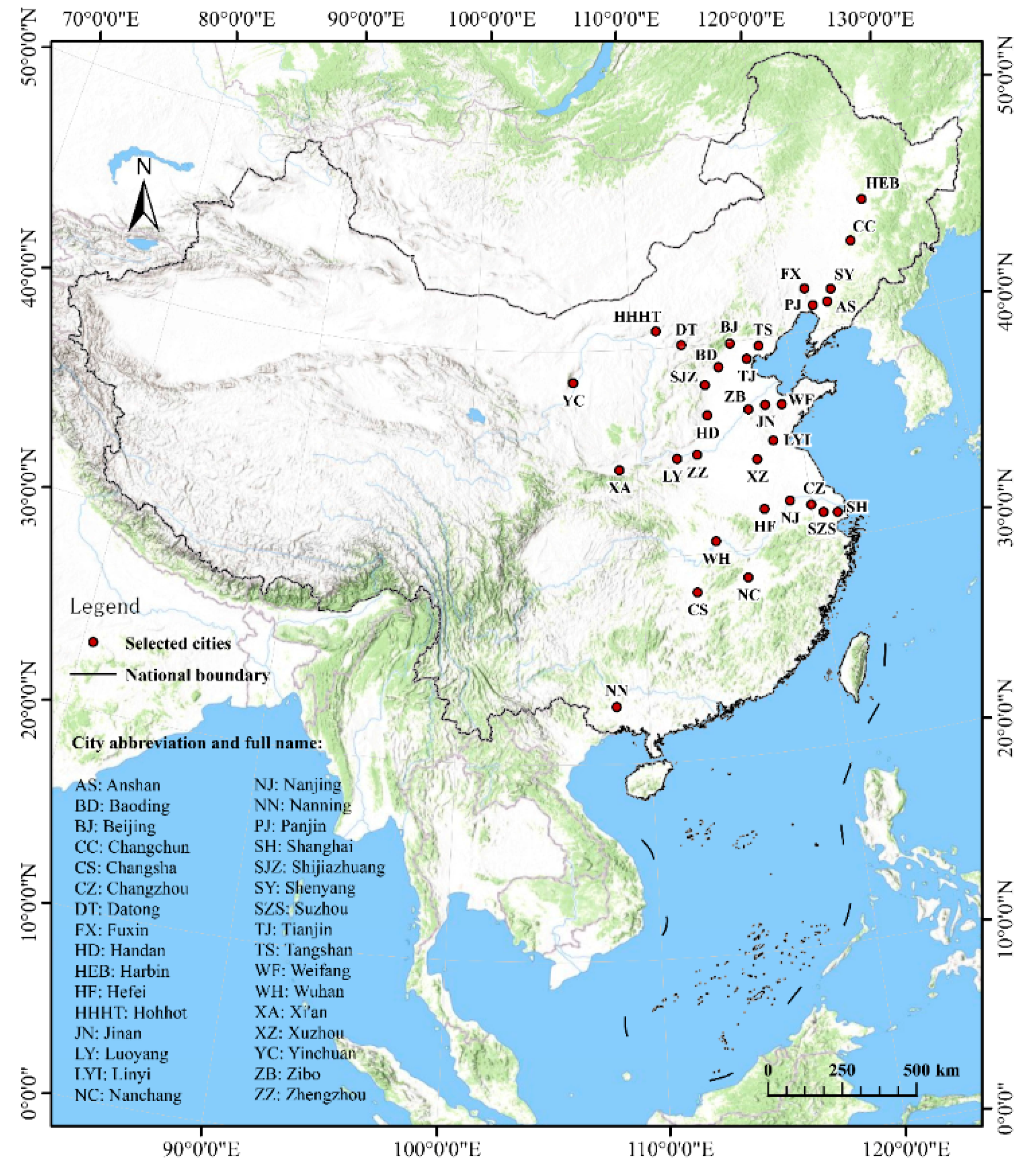
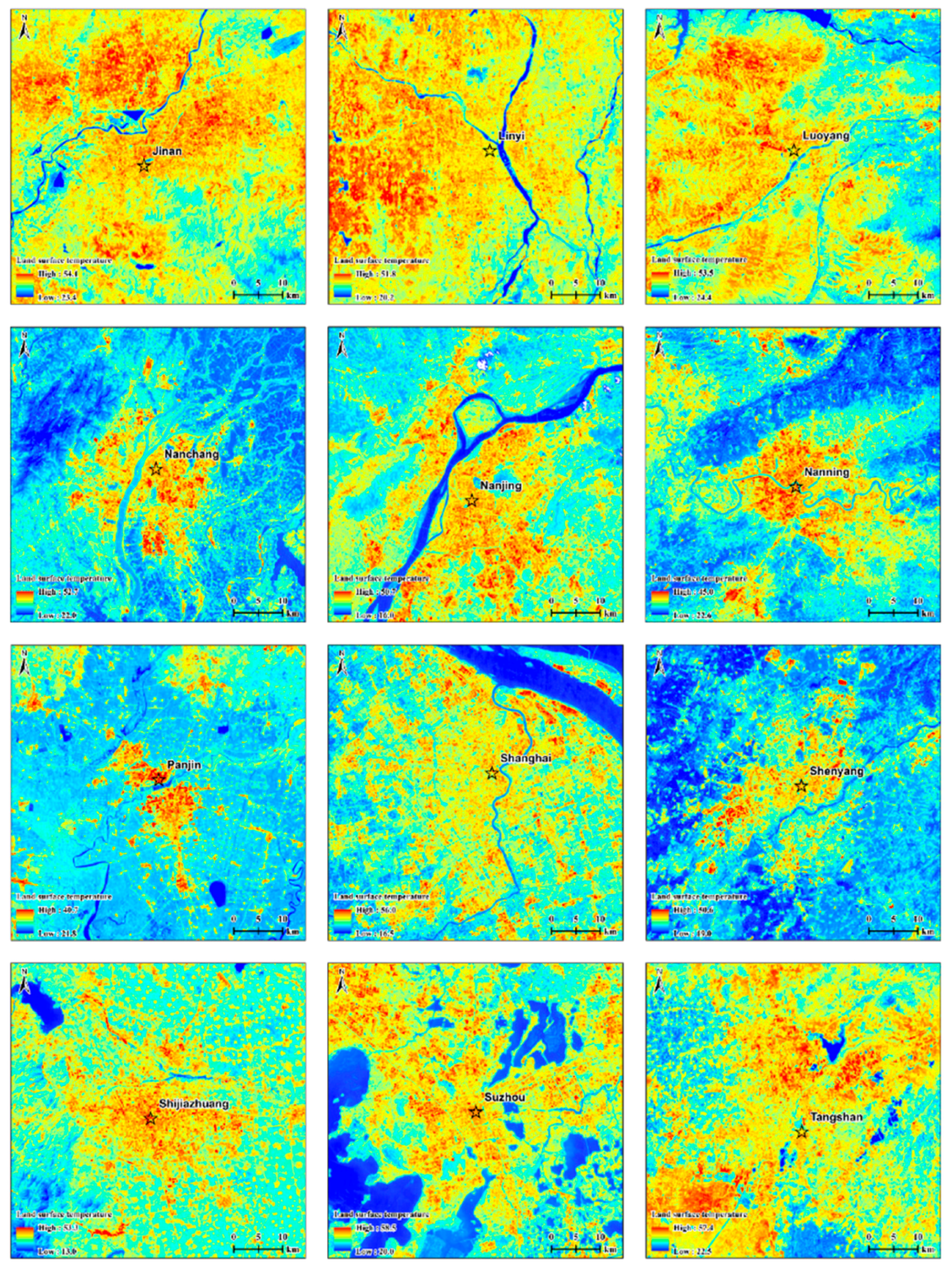
2.1. Study Areas and Data Pre-Processing

For our study, we selected major Chinese cities with built-up areas >100 km2 in 2015. For this selection, as a first step, we extracted all built-up areas within China using the global land cover product at a spatial resolution of 300 m from the Climate Change Initiative of the European Space Agency (ESACCI-LC-L4-LCCS-Map-300m-P1Y-2015-v2.0.7) [32]. By filtering out those <100 km2, we yielded 70 candidate cities. The social sensing data were real-time data and we collected it in October 2017, so we checked all available cloud-free Landsat-8 OLI images acquired during 2015–2017 to ensure the time-efficiency of the data. Eventually, 32 cities that had available cloud-free images during this time period were defined as our study areas (Figure 1, see Table A1, Appendix A for detailed information). All Landsat-8 images used in this study were geometrically registered. For each image, we conducted radiometric calibration and then atmospheric correction using the FLAASH tool with the ENVI 5.2 software. The resulting reflectance images were used for subsequent analyses.

2.2. Land Surface Temperature Retrieval

We used the radiative transfer equation (RTE) algorithm [33] for the Landsat-8 thermal infrared sensor (TIRS) to quantitatively retrieve the LST in all studied cities, considering that the accuracy of this algorithm has been repeatedly validated [8,17]. A brief description of the RTE algorithm is given below:
L λ = [ ε B ( T S ) + ( 1 ε ) L d ] τ + L u ,
where Lλ is the apparent radiance received by the sensor; ε is the surface emissivity; Ts is the land surface temperature; B ( T S ) is blackbody spectral radiance; τ is atmospheric transmittance; L u is the upwelling path radiance; and L d is the downwelling path radiance. According to Plank’s Law, B ( T S ) can be calculated as:
B ( T S ) = [ L λ L u τ ( 1 ε ) L d ] / τ ε ,
Then, the LST ( T S ) can be calculated as:
T S = K 2 / ln ( K 1 / B ( T S ) + 1 ) ,
The atmospheric parameters τ , L u , and L d can be calculated with the Atmospheric Correction Parameter Calculator [34]. For Landsat-8 TIRS band 10, K 1 = 774.89   mWm 2 s · r 1 μ m 1 ; K 2 = 1321.08   K .
The retrieved LST maps can be found in Appendix A (Figure A2).

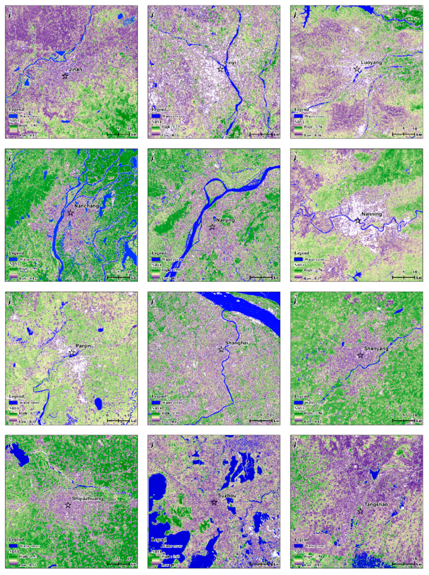
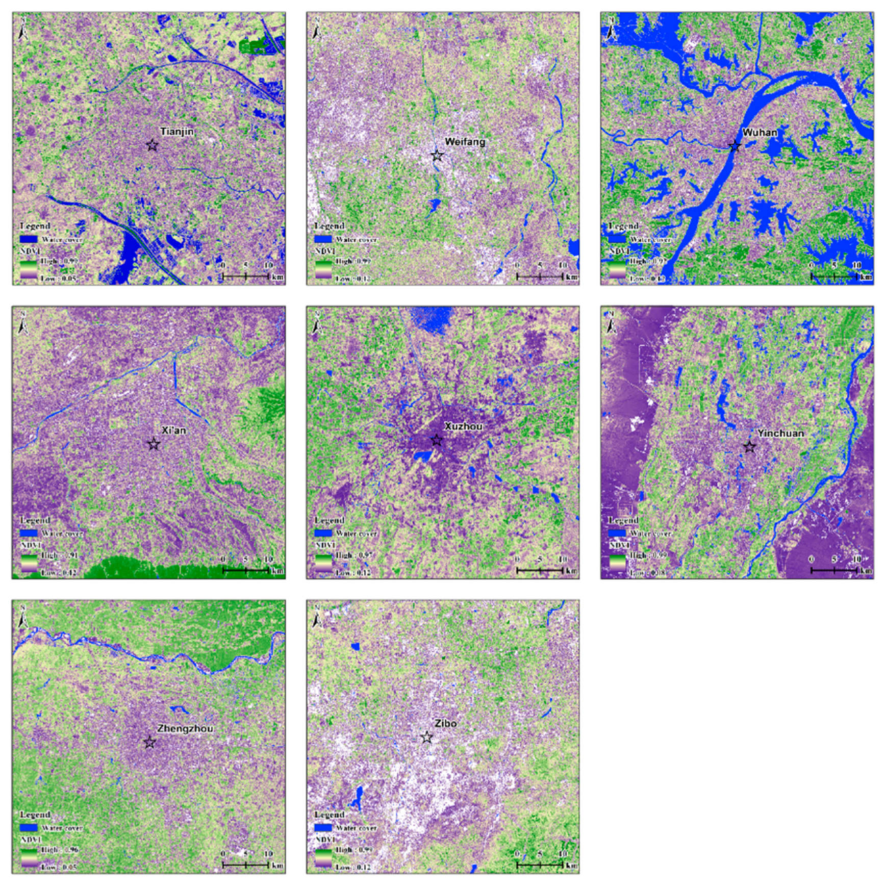
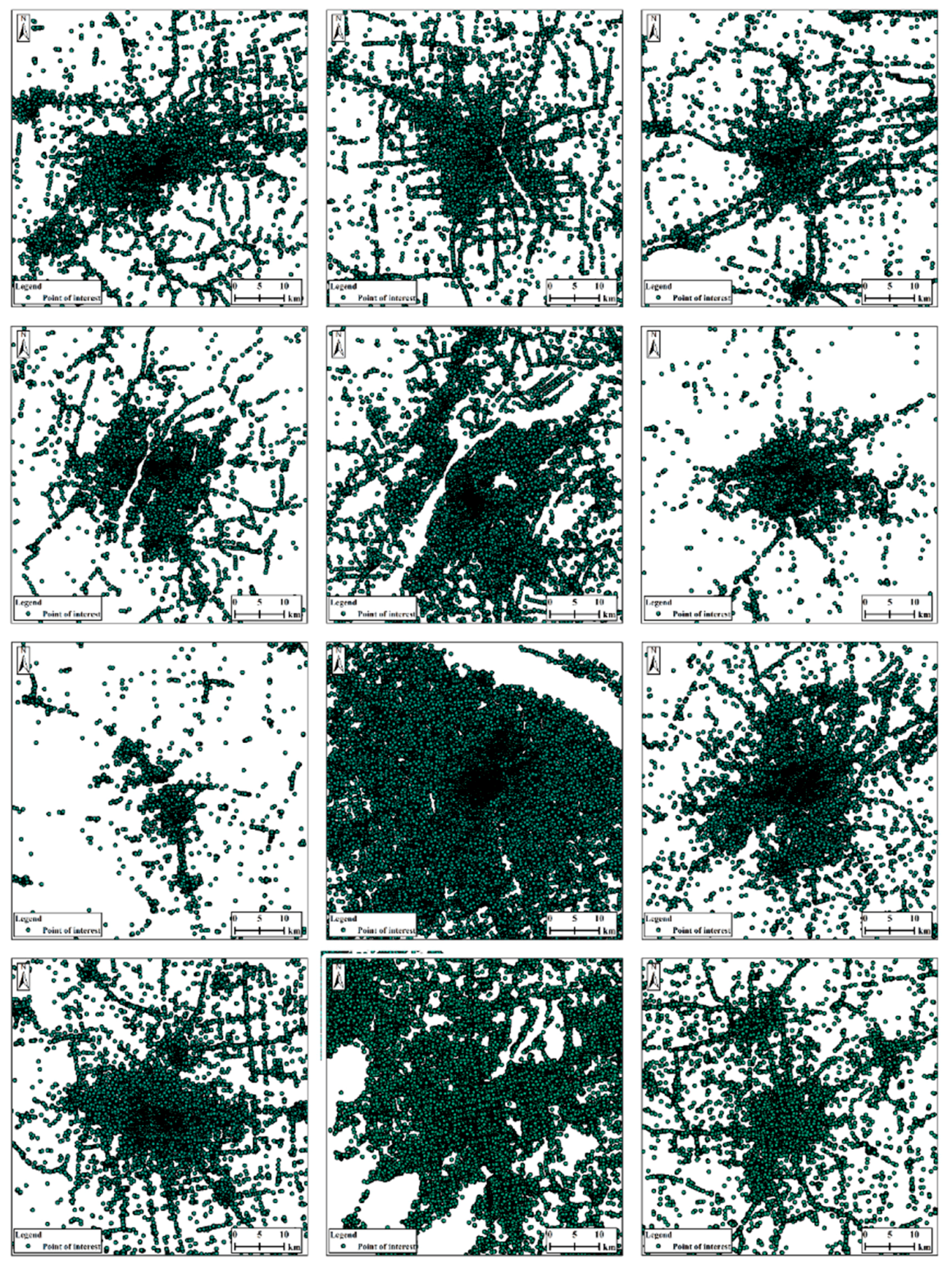
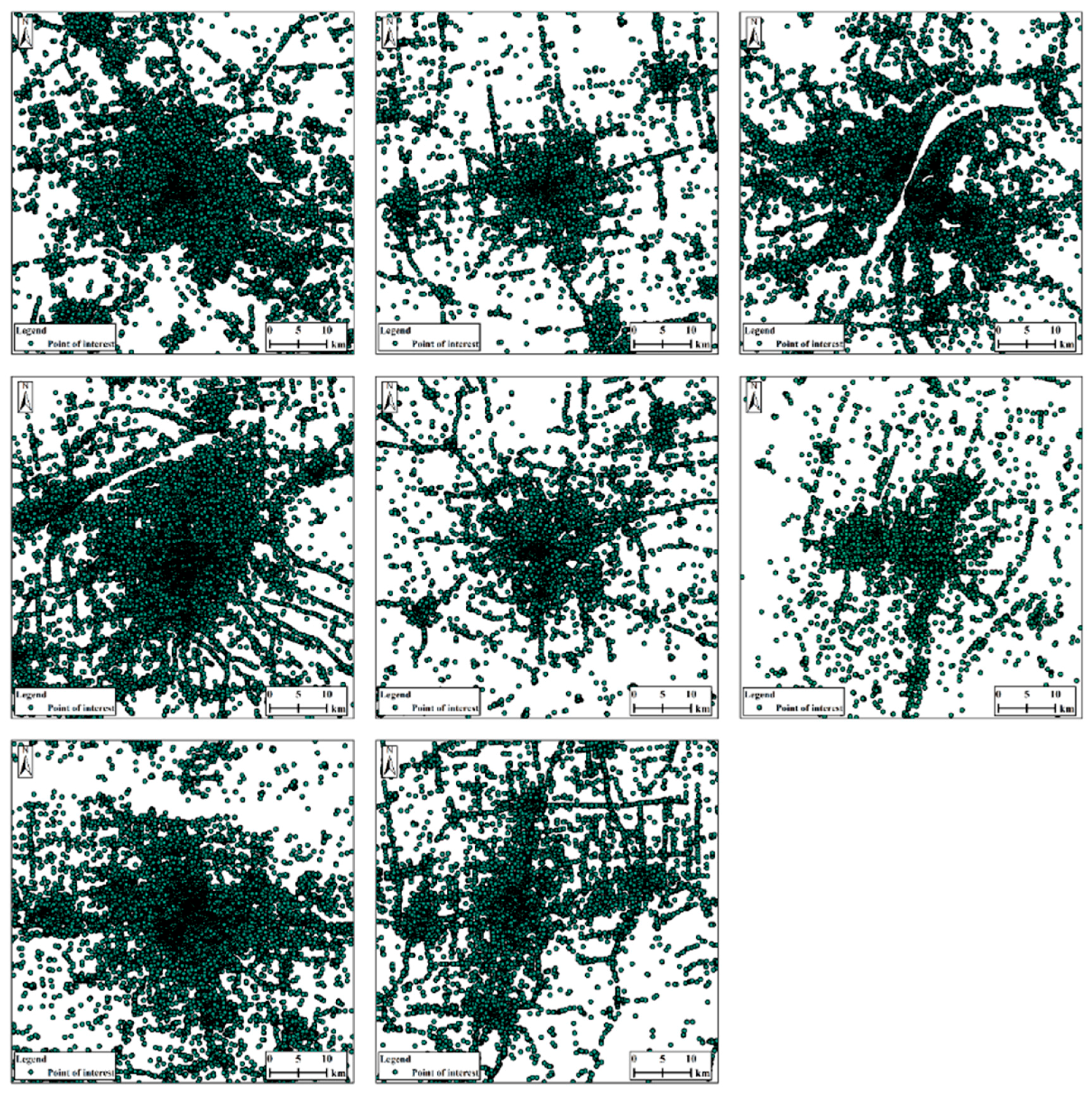
2.3. Natural-Surface and Non-Surface Variables

Prior to analyses, the areas were divided into grid cells at a particular size (see Section 3.2 below). Within each grid cell, we calculated the natural-surface and non-surface variables. Our natural-surface variables included vegetation cover and water cover (seen in Figure A3, Appendix A) as they are the most commonly used variables in the studies of the surface UHI effect [4,14,19,35]. Within each grid cell, we calculated the mean of the normalized difference vegetation index (NDVI) for all vegetated pixels as an indicator of vegetation cover. For water cover, we calculated the percentage of water bodies within each grid cell.
We used POI as an indicator of the intensity of human activities. POI is a point type geo-located data representing all urban facilities such as companies, shopping malls, schools, and parks. Unlike traditional remote sensing data where one building is one point, POI data can give more detailed information within the building such as the shops, restaurants, beauty shops, etc. close by. More POI density means more human activity intensity. POI data are real-time data and we collected the data in October 2017. The POI data were obtained from the AMap [36], which is one of the most widely used web mapping and navigation services in China. We derived the spatial data of POIs for each studied city using the application programming interface (API) provided by AMap (Figure A4, Appendix A). We then calculated the density of POIs within each grid cell.

3. Methodology

3.1. Statistical Analyses

To assess the explanatory power of the natural-surface vs. non-surface variables, we constructed regression models with LST as the response variable and NDVI, water cover, and POI density as the explanatory variables (one grid cell represents one data point in the models). NDVI, water cover, and POI density were log-transformed to approach normal distributions before model fitting.
As a first step, we constructed the most commonly used univariate ordinary least squares (OLS) models to assess the explanatory power (measured by R2) of each individual explanatory variable in explaining the observed LST patterns [28,37]. Then, we combined all three explanatory variables to fit multivariate OLS models to assess their collective explanatory power (measured by adjusted R2). We used the relative importance analysis (RWA) to partition the relative importance (measured by the proportional contribution of the variables decomposed from the total explanatory power) of the three explanatory variables [38]. In addition, to account for the potential spatial autocorrelation (SAC) problem in the OLS models, we used simultaneous autoregressive (SAR) models to test for the robustness of our results. We used the spatial error model (SARerr) recommended by Kissling and Carl [39], considering the uncertainty of the autocorrelation sources [40,41]. The explanatory power of the SAR models was decomposed into spatial signal versus non-spatial trends. We subsequently calculated the pseudo-R2 of the non-spatial component, and by checking the result of the SARerr model for explaining the LST pattern (Figure A19, Appendix B), we found that our OLS scaling relations were qualitatively robust to spatial autocorrelation. Considering that a comparison with other studies where the OLS model was mostly used as well as the method for the application of the RWA to SAR models are not available yet, we only used the results of the OLS model to answer our questions in this article. The statistical analyses were performed with R 3.3.4. The RWA was performed by using the RWA-Web software [42].

3.2. Scaling Analysis

We conducted a straightforward scaling analysis by systematically varying both the spatial extent and grain size to quantify the individual explanatory power of NDVI, water cover, and POI density as well as their collective explanatory power at different spatial scales. In doing so, for each city, we restricted the study area within a squared region according to the urban areas, and then divided this squared region into grid cells; we changed the size of the squared region (i.e., 20 × 20 km2, 30 × 30 km2, 40 × 40 km2, 50 × 50 km2, and 60 × 60 km2) for the varying spatial extent, and changed the size of the within grid cells (i.e., 0.25 × 0.25 km2, 0.5 × 0.5 km2, 1 × 1 km2, 2 × 2 km2, and 5 × 5 km2) for varying grain size (see Figure A1, Appendix A for the schematic diagram of the scaling analysis). For the selection of the spatial grain size, 500 m and 1000 m are the most commonly used grain sizes for the study of the UHI effect and so we made the scaling ladder approximate a double geometric progression that could be divisible by the spatial extents. At each combination of spatial extent and grain size, we conducted all the statistical analyses (in Section 3.1) and the scaling relations were assessed by looking at how the explanatory power changed across the scale ranges.
The materials used, data processing, and the procedures carried out are shown in the flowchart below (Figure 2).

4. Results

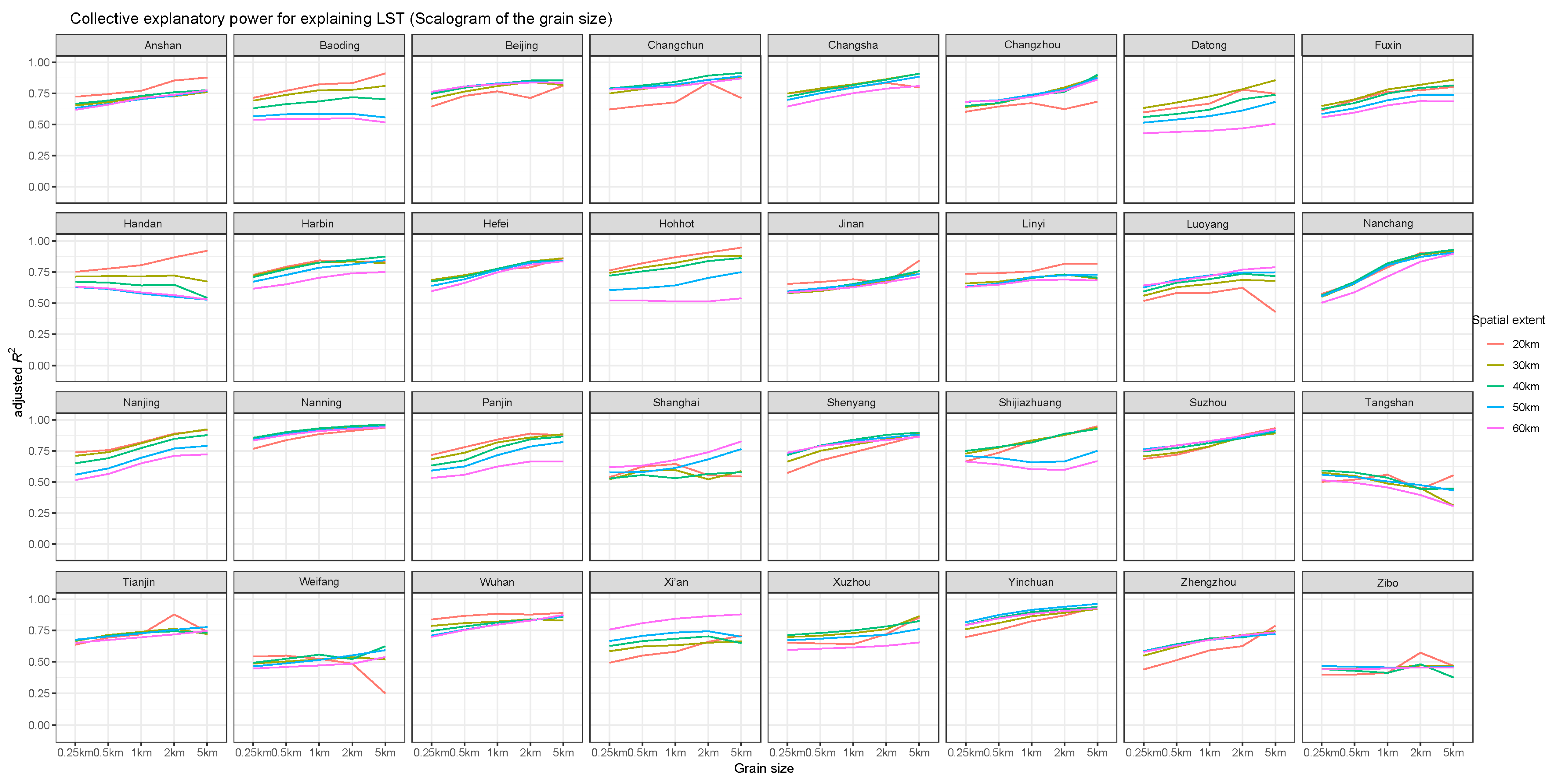
4.1. Scaling Relations at the City-Collective Level

The natural-surface (NDVI and water cover) and non-surface (POI density) variables jointly explained a considerable proportion (ca. 50–90%) of LST variance for all studied cities (Figure 3), suggesting that they are indeed good predictors of the UHI patterns. Our scaling analysis clearly demonstrated that for the selected variables, both separately and collectively, their explanatory power was strongly dependent on the spatial scale with respect to both grain size and spatial extent. At the city-collective level (aggregating all studied cities), the adjusted R2 of the full model with all three variables included demonstrated an increasingly linear-like (close to monotonic) scaling relation as the grain size coarsened from 0.25 km to 5 km (Figure 3a), and a decreasingly linear-like scaling relation as the spatial extent was enlarged from 20 km to 60 km (Figure 3e).
The results from the individual variables revealed that their strengths in shaping the UHI patterns were also strongly scale-dependent at the city-collective level (Figure 3). With changing grain size, the strengths of the NDVI and POI density (measured by the adjusted R2 of the univariate models) showed linear-like scaling relations (Figure 3b,d), which was similar to that of the total strength of all three variables (Figure 3a). However, their scaling relations with respect to spatial extent tended to exhibit hump-shaped patterns, which were clearly different to the total strength (Figure 3e). In contrast with the NDVI and POI, water cover had weaker strength, and its scaling relations with respect to both grain size and spatial extent seemed to have similar trends with (though more erratic than) those of the total strength (Figure 3c,g).
Among the three individual variables, NDVI generally had the highest relative importance at all spatial scales (Figure 4a), suggesting that vegetation cover is a dominant determinant of UHI patterns. Water cover and POI density appeared to have comparable relative importance at the city-collective level. We also observed a clear scale dependency of the relative importance of the variables. With increasing grain size, the relative importance of POI density gradually increased and exceeded that of water cover at coarse grain sizes of 2 km and 5 km. Moreover, we observed a strong scale dependence of the relative importance of the three variables. Generally, the relative importance of all three variables had linear-like scaling relations with respect to grain size (Figure 4a–c): the relative importance of NDVI and water cover declined while that of the POI density was elevated with coarsening grain sizes. With respect to spatial extent, in general, the relative importance of NDVI and POI presented a hump-shaped scaling relation, while water cover showed an inverse humped scaling relation.

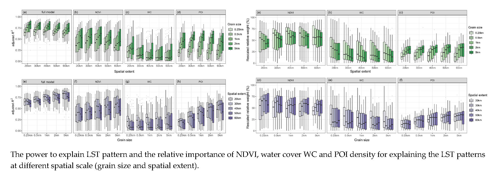
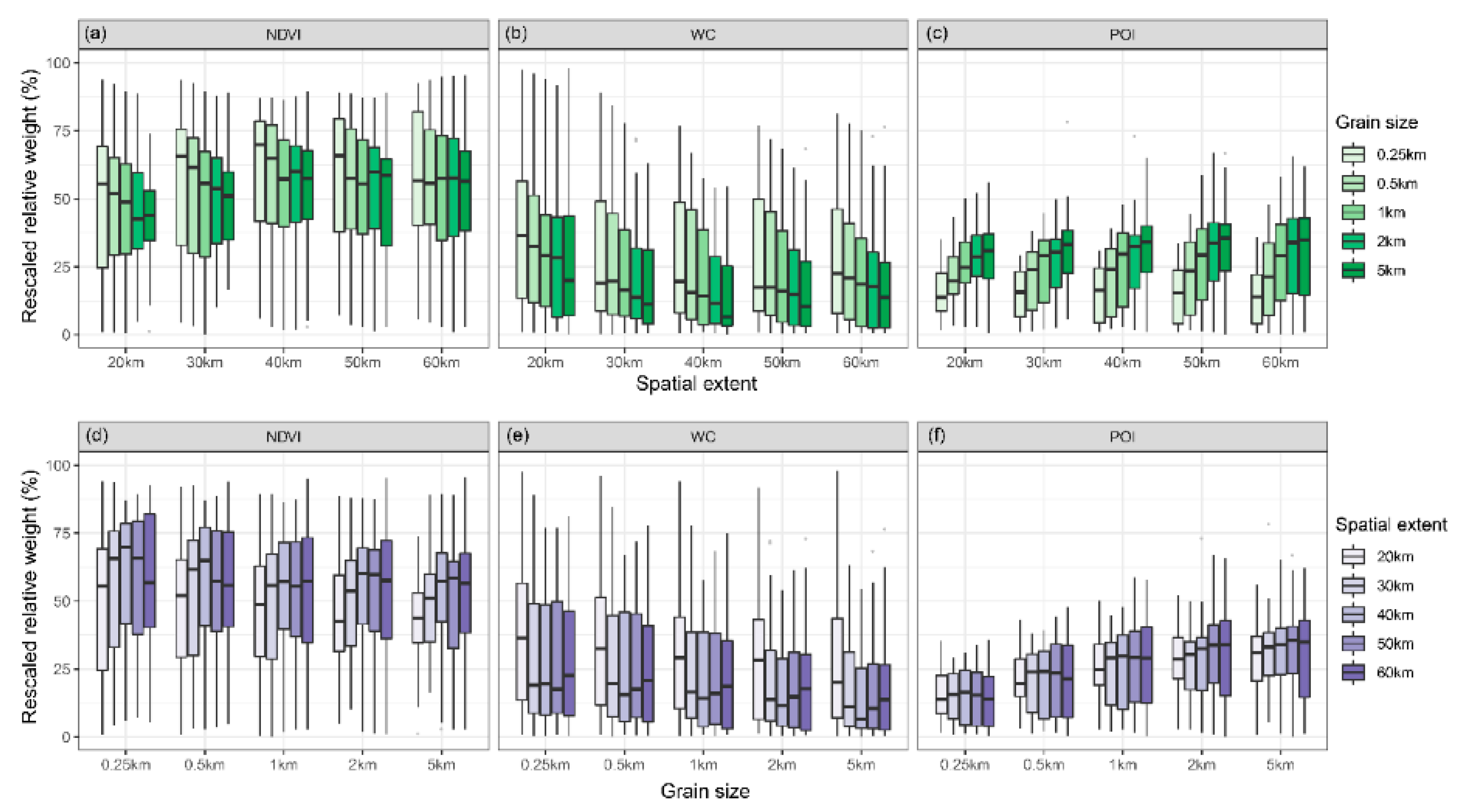
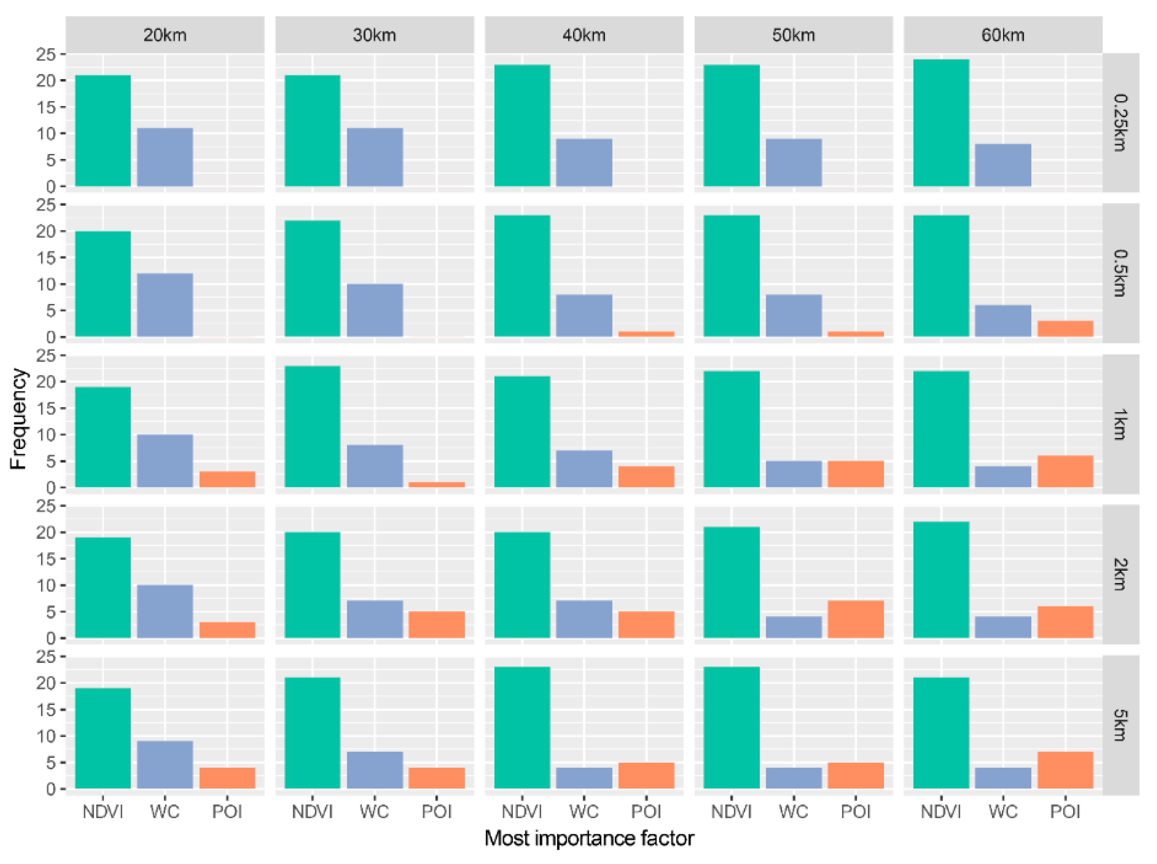
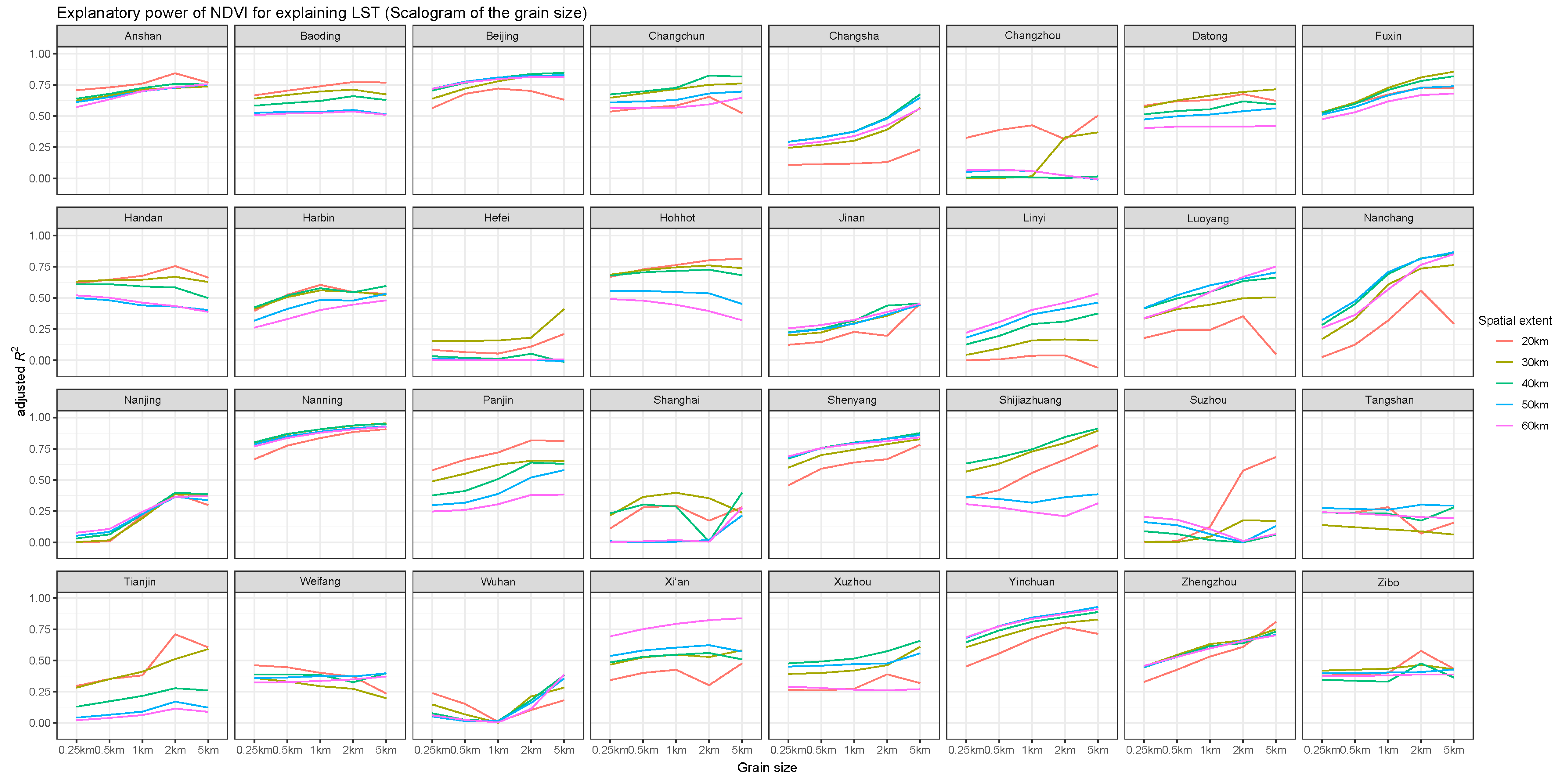
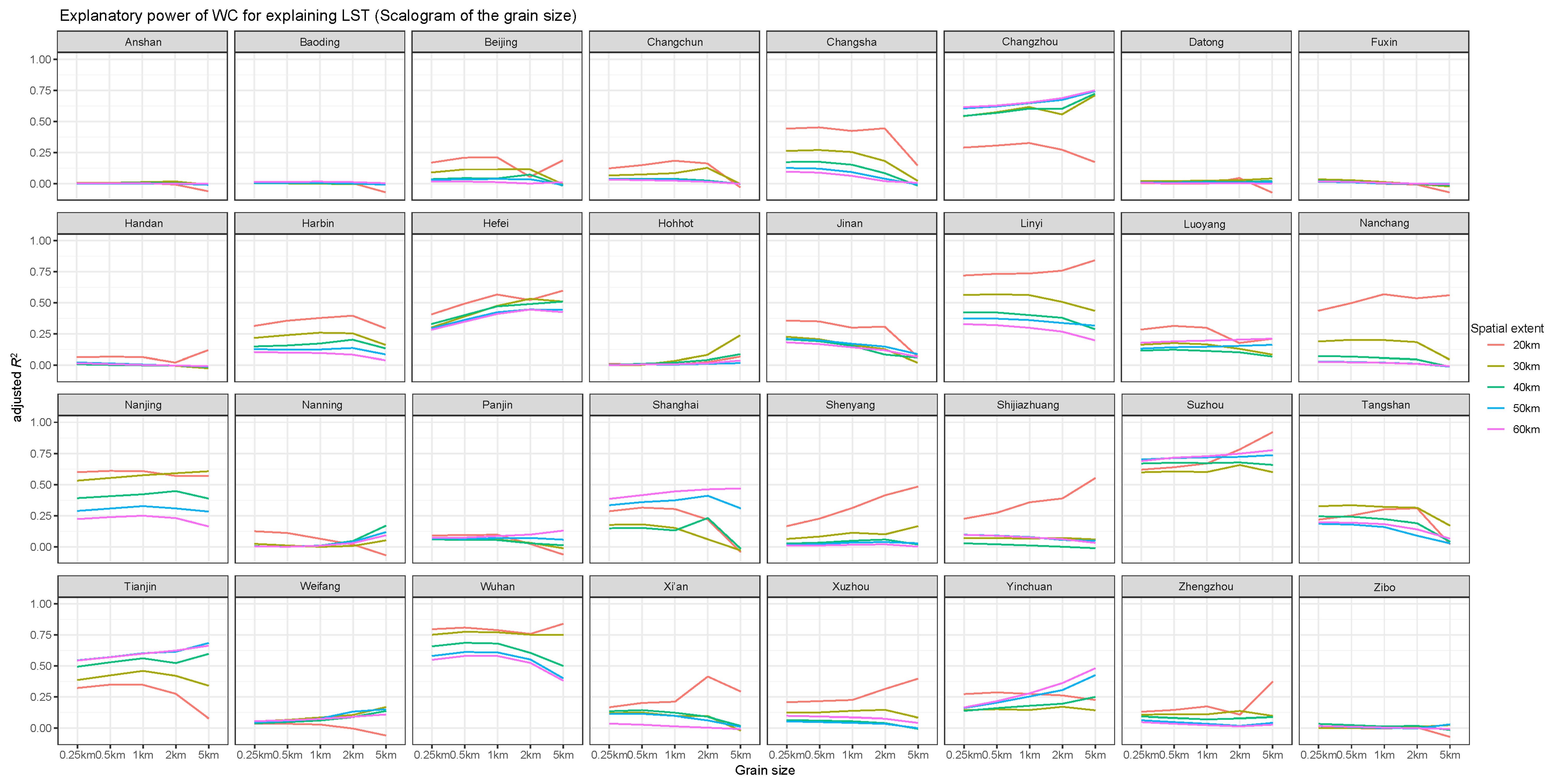
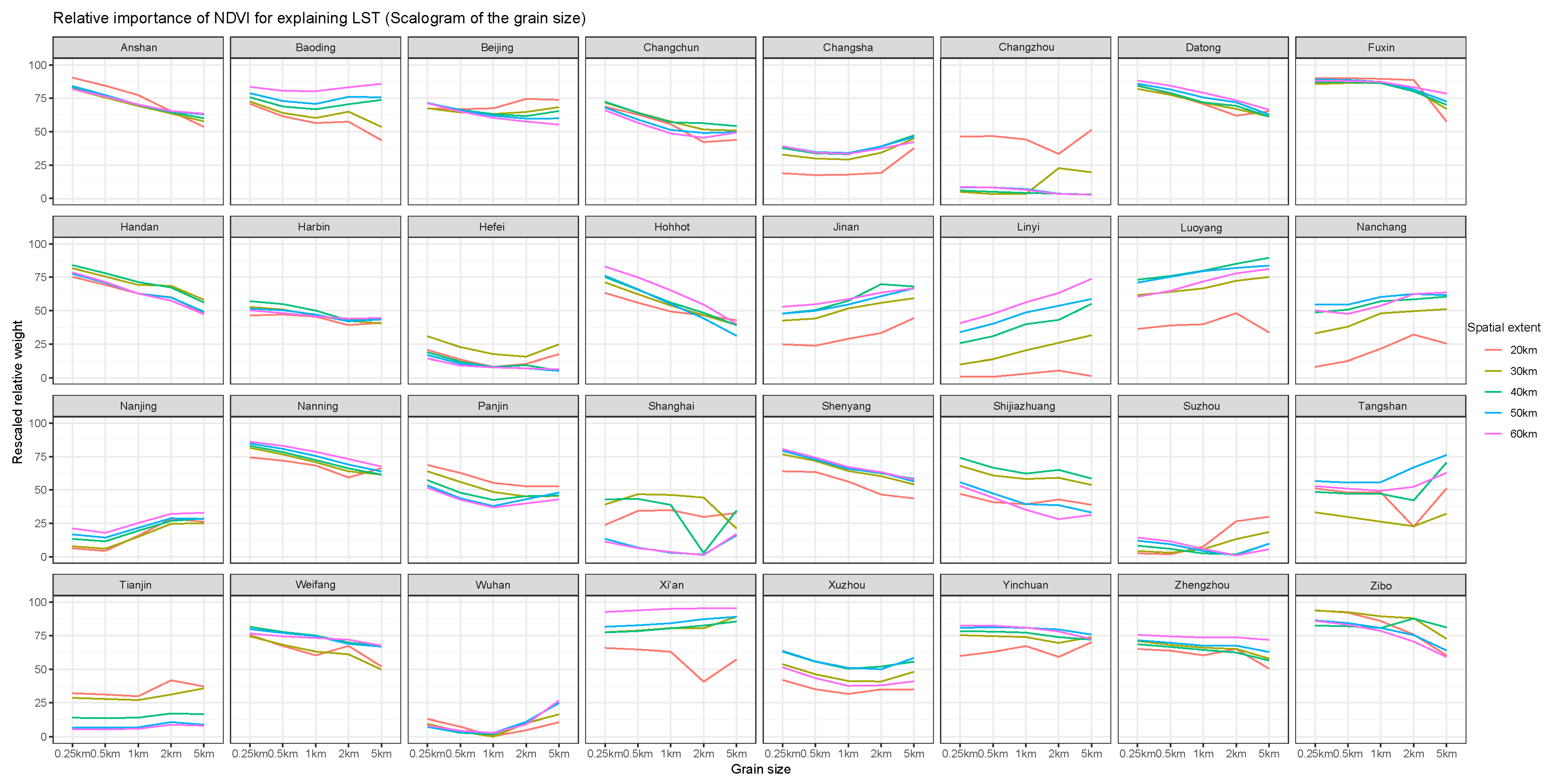
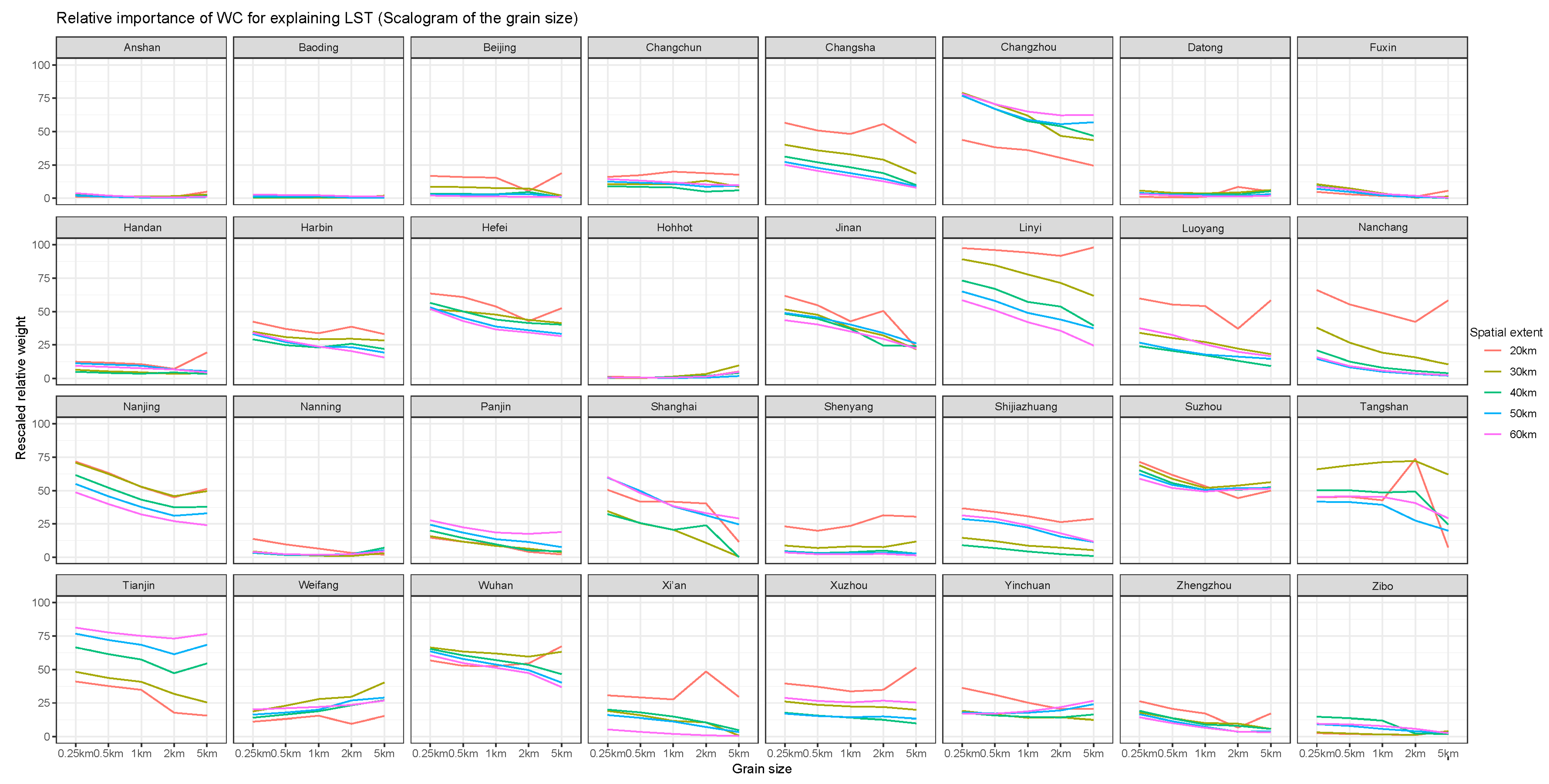
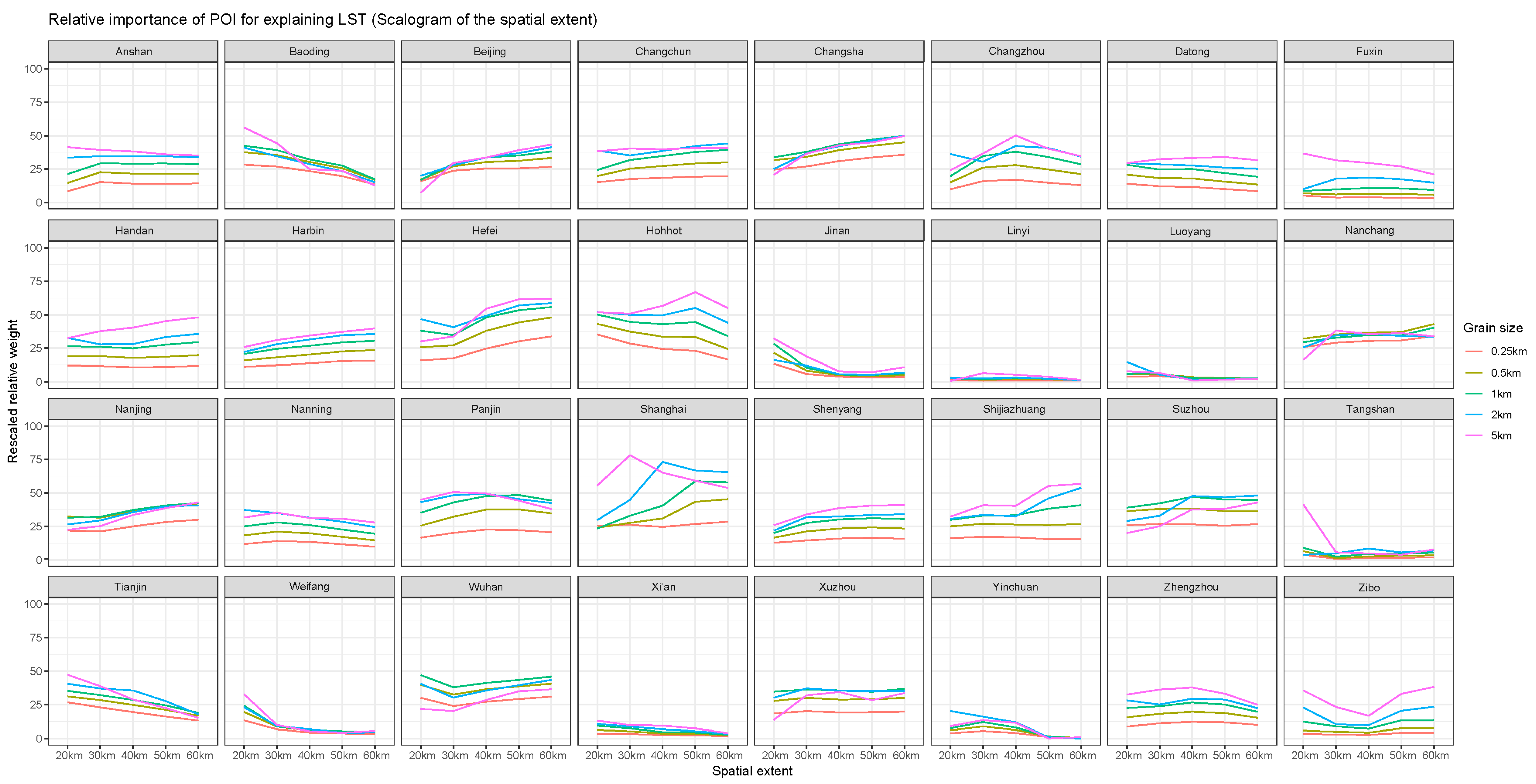
4.2. Scaling Relations and Variable Relative Importance at the Individual-City Level

While the above-mentioned city-collective-level analysis clearly revealed the general scaling patterns, it remains unclear whether or not such ‘aggregated’ patterns have resulted from consistent scaling behavior across different studied cities. We then closely scrutinized each individual city. Comparted with the linear (monotonic) scaling relations that were mostly found at the city-collective level, we observed much more diverse scaling relations at the individual-city level. Specifically, we identified six types of scaling relations, referred to as (1) monotonically increasing, (2) monotonically decreasing, (3) humped, (4) inversely humped, (5) scale invariant, and (6) erratic (Figure 5). The monotonic increasing or decreasing scaling relations were often the most frequent types across the individually studied cities (Figure 5 and Figure 6, detailed scaling relations for each city could be found from Figure A5, Figure A6, Figure A7, Figure A8, Figure A9, Figure A10, Figure A11, Figure A12, Figure A13, Figure A14, Figure A15, Figure A16, Figure A17 and Figure A18 in Appendix B), giving rise to the general scaling patterns at the collective-city level. However, very contrasting scaling relations can also frequently arise. For example, the strength of the NDVI had both monotonic increasing and humped scaling relations with respect to grain size at the spatial extent of 20 km (Figure 5b, green bars). Our results thus demonstrate that the strengths of the UHI determinants as well as their relative importance can vary from city to city, suggesting that the scaling relations are clearly system-specific.
To further illustrate the system-specificity of the relative importance, we plotted the number of cities that were found to have NDVI, water cover, or POI density as the most important determinant at a given spatial scale (Figure 7, see Table A2, Appendix B for detailed information). The NDVI was consistently identified as the dominant determinant in ca. 20 cities (around 60%) across all observational scales; water cover was identified as the dominant determinant in up to 12 cities (i.e., ~35% of the studied cities); and POI density as the dominant determinant in up to seven cities (i.e., ~20% of the studied cities). An interesting pattern is that the dominance of POI density tended to be more pronounced at coarser grain sizes and larger spatial extents. In brief, the natural-surface variables were the most important UHI determinates, but the non-surface variable can occasionally dominate the UHI patterns, especially at larger spatial scales.

5. Discussion

5.1. Scale Dependency and System Specificity of Urban Heat Island Determinants

Our study demonstrates that the strengths of the UHI determinants as well as their relative importance are strongly dependent on the observational scale and are clearly system-specific. This is not very surprising in the sense that scale dependency and system specificity are generally expected to occur, and have been found in many geographic, ecological, and social patterns [30,31,43]. However, the remarkably high plasticity of the UHI determinants (to spatial scale and studied system) revealed by our analyses was indeed unexpected. For example, when comparing different spatial scales, we found up to a threefold difference in the assessed strength of particular determinants for the same city (see figures in Appendix B); and this difference can be even larger when comparing different cities. Such plasticity may easily lead to contrasting conclusions if the observation is based on a single scale and a single city, as in many previous studies [15,28,31].
A general scaling relation we found was that the selected natural-surface and non-surface variables, collectively, could better explain the observed LST patterns at smaller spatial extents, but coarser grain sizes. These detected scaling relations might be underpinned by the spatial heterogeneity of LST. With increasing spatial extent, the thermal environment would generally present higher spatial heterogeneity (caused by more heterogeneous topographic conditions, background climatic conditions, etc.) associated with more coexisting determinants and/or shaping mechanisms of UHIs [7,44,45]. When the grain size becomes finer, the local-scale variation of thermal conditions will become stronger as a result of increasing heterogeneity of micro-environment in terms of the spatial configuration of the buildings [10,46] three-dimensional (3D) vegetation structure [47,48], and other factors. These heterogeneities may not be well captured by our selected variables and/or single linear models, leading to declined explanatory power.
For the individual variables, we found that the explanatory power of NDVI increased monotonically as the grain size became coarser. This finding is in line with some previous studies [11,49,50], but contradictory to others [26,44,51,52]. For instance, Weng, Lu, and Schubring [51] and Liu and Weng [52] suggested that the detected relationship between LST and NDVI was strongest at an intermediate grain size of 120 m in Indianapolis City, USA. While we cannot be certain whether this contradiction results from the different data sources and analysis methods used, it is very likely that it is attributed to system-specific scaling relations, because humped scaling relations of the NDVI were also found in some Chinese big cities in our study (Figure 5b). It has been documented that water bodies have a cooling effect [18,35,53], however, the scaling relations of water cover are not really clear. This multi-scale analysis revealed that 20 km is the threshold spatial extent for understanding the contribution of water cover to the LST pattern (Figure 3g), which further deepens the understanding of the contribution of water cover to LST and its cooling effect. Furthermore, we demonstrated that POI density can contribute to the formation of LST patterns and that its contribution increases with coarsening grain size.
In addition, studies on the formation mechanisms of LST patterns have mostly focused on particular influencing factors, leaving their relative importance poorly understood thus far, especially at different scales [13,26,48]. Natural surfaces and human activities can largely explain the LST pattern that was also demonstrated in this study, while the relative importance between both of them is controversial, as we stated above (see also in the Introduction). Through this multi-scale analysis, we found that the relative importance of green vegetation to LST was the highest at all spatial scales for the city-collective level, and it was significantly higher than the water cover and human activity intensity. This finding provides new evidence that the natural surface contributes more to the LST pattern than human activity [3,29]. However, the relative importance of water cover and POI to the LST shows different results at different scales (Figure 3). In contrast to the trend of human activity on the LST, the relative importance of water cover decreased with increasing grain size, and the spatial extent of 20 km is a threshold because the relative importance of water cover decreased significantly when the spatial extent exceeded 20 km (Figure 3). These results challenge our past understanding that the contribution of water cover to the LST generally increases with spatial scale, while the contribution of human activities to the LST is usually greater on a smaller spatial scale [6,26,35,53].

5.2. Implications

Many previous studies have demonstrated that green vegetation has a significant cooling effect, and the cooling effect can vary depending on the type of green vegetation, spatial pattern (composition and configuration) of green vegetation [12,17,18,49], and local background climate [54]. Our findings revealed that vegetation cover generally has the largest strength in shaping the LST patterns at most of the studied scales and lends support to previous argument that the natural surface contributes more to the LST pattern than human activity, and highlight the importance of green vegetation (and nature-based solution) for city planning in the context of climate adaptation [12]. In contrast, some case studies have found that the cooling effect of the water body was better than the green vegetation due to the higher rate of the heat consuming process of transpiration [14,54]. Our results suggest that this is also possible, as for the single-city level, the results of many cities showed that the water body was the dominant factor to explain the LST pattern, especially at finer spatial scales (Figure 6). This further indicated that the explanatory power and relative importance of the selected variables are largely scale-dependent and system-specific. Nevertheless, the results of the water body (Figure 2g and Figure 3e) indicate that decision makers or planners can design water bodies on a smaller spatial grain and extent (20 km) to mitigate the UHI effect.
The study also showed that as the grain size and spatial extent increases, human activities can contribute to the LST pattern more (Figure 3 and Figure 6). This result suggests that reducing anthropogenic heat emissions is an optional measurement for climate mitigation. In particular, the urban agglomeration has become the most salient feature of global urbanization in recent decades, hence regional thermal environment mitigation has increasingly become the focus of policy attention. In addition, the results of this study also showed that compared with the cooling effect of green space and water body, the relative importance of human activities to LST was not that significant, especially at finer spatial scales (Figure 3 and Figure 6). Therefore, according to these findings, the implication could be that compared with restricting human activities induced anthropogenic heat emissions, planning more green vegetation (and water bodies) is more efficient for climate adaption.
Overall, this study demonstrates that natural surfaces and human activities can largely determine the LST pattern and that human activity has a positive effect on the increase in LST (SUHI). On the other hand, to mitigate the UHI effect, we suggest that green vegetation (or nature-based solutions) is the best way to cool cities and urban agglomerations. Moreover, from a larger perspective, we would like to mention again the classic problem of landscape ecology–scale effect, that is, the patterns and process relationships found in one system or one scale may not be applicable to another system or scale. This study once again makes us notice the role of scale effects in other disciplines.

5.3. Limitations and Further Studies

Some limitations need to be mentioned in this study. First, due to image resolution limitations, only five grain sizes from 0.25 km to 0.5 km were selected for this study. The city is a region with a very high degree of landscape heterogeneity, so a high resolution of grain size is needed to obtain more detailed information in follow up studies. At the same time, urban agglomeration has become the most salient feature of urbanization in recent decades, so larger spatial scale-based studies are also needed to provide valuable implications for climate adaption in urban agglomerations [8,16,55]. Second, previous studies have found that LST patterns vary between day and night and vary in different seasons and climate zones. This study only used daytime thermal images to undertake the study and did not take the background climate into account. Although the 32 selected Chinese cities had similar meteorological conditions (e.g., temperature and relative humidity) in the summer season, it would be better if we could take the background climate into consideration in future studies. Therefore, future research should also further analyze the daytime and nighttime differences and seasonal differences. Third, more detailed human activity data and the 3D structure of the city need to be further considered. With the rapid development of information technology, more and more human activity data have appeared, so we should try to use these more detailed and new data for further research. Furthermore, urban 3D morphology also has effects on the LST pattern, but this study did not consider the effects of urban 3D structure, which may underestimate the impact of human activities on land surface temperature, particularly on air temperature.
In addition, although this study revealed the scale effect of the contribution and relative importance of natural surfaces and human activities to the LST pattern as well as suggest implications for climate adaption planning, the study still does not provide more valuable information such as how much green vegetation and water should be placed on a given spatial scale to most effectively reduce UHIs. Therefore, more research is needed to find the thresholds for the composition and configuration of green vegetation and water cover on a given spatial scale.

6. Conclusions

Taking 32 selected Chinese cities as the sample, this study examined the scale (spatial extent and grain size) effects of the contribution and relative importance of natural surfaces and human activities to the UHI pattern. The study revealed that the contribution and relative importance of natural surfaces and human activities are highly dependent on the scale-dependent and system-specific strengths. Specifically, this study found the following. (1) The full model of natural surfaces and human activities had a higher contribution to LST at all spatial scales generally, and the explanatory power and relative importance of natural surfaces and human activities are scale-dependent and system-specific. (2) The green space is negatively correlated with the LST pattern and showed more dominance than water and human activity intensity at all spatial scales, which implies that green vegetation (or nature-based solutions) is the best way to cool cities and urban agglomerations. (3) The water cover is significantly negatively correlated with the LST and the relative importance of water cover decreases with increasing grain size, and the spatial extent of 20 km is a threshold. Contrary to the water body, human activities are significantly positively correlated with the LST and as the spatial extent and grain size increase, human activities can contribute to the LST pattern more. These results can guide planners to plan water bodies on a smaller spatial grain and extent (20 km) to mitigate the UHI effect. Additionally, when conducting climate adaptation planning on a larger spatial scale, we should pay attention to reducing anthropogenic heat emissions, especially at a regional (urban agglomeration) scale. The study expands the understanding of the LST formation mechanisms at a different spatial scale and different cities, and its methods and results provide useful insights into thermal environment research and practice.

Author Contributions

Conceptualization, Z.Y., X.L., and C.X.; methodology, X.L. and C.X.; processing and analyses of data: X.L., Y.Z., S.W. and X.M.; visualization, X.L.; writing—original draft preparation, X.L., Z.Y.X.H., and Z.Y.; writing—review and editing, Z.Y., S.N.T. and C.X.; supervision, Z.Y., S.N.T. and C.X. All authors have read and agreed to the published version of the manuscript.

Funding

This research was funded by the National Natural Science Foundation of China (grant no. 31770512), the Open Foundation of the State Key Laboratory of Urban and Regional Ecology of China (grant no. SKLURE2019-2-6), the Shanghai Key Lab for Urban Ecological Processes and Eco-Restoration (grant no. SHUES2019A01); and the WEL Visiting Fellowship Program. CX acknowledges the support from the CTF Foundation.

Acknowledgments

Chi Xu (xuchi@nju.edu.cn) and Shuqing N. Teng (shuqingteng@nju.edu.cn) are also corresponding authors of this paper. We also thanks anonymous reviewers for their constructive comments and suggestions.

Conflicts of Interest

The authors declare no conflict of interest.

Appendix A

Table A1. List of the cities and the path/row numbers and the time of the Landsat 8 images each city used.
CityPath/RowTimeCityPath/RowTime
Anshan119/312017.08.31Panjin120/312017.09.07
Baoding123/33;2017.07.10;Shanghai118/38;2017.08.24;
124/332017.07.01118/392017.08.24
Beijing123/322017.07.10Shenyang119/312017.08.31
Changzhou119/382017.05.27Shijiazhuang124/33;2016.08.31;
124/342016.08.31
Datong125/322017.08.25Suzhou119/382017.05.27
Fuxin120/312017.09.07Tangshan122/32;2017.06.01;
122/332017.06.01
Harbin118/282017.07.07Tianjin122/332015.06.12
Handan124/34;2016.08.31;Weifang121/34;2017.07.12;
124/352016.08.31121/352017.07.12
Hefei121/382016.07.25Wuhan123/392016.07.23
Hohhot126/322017.06.29Xi’an127/362016.06.17
Jinan122/34;2015.06.12;Xuzhou121/36;2015.06.05;
122/352015.06.12122/362015.07.30
Linyi121/362017.05.25Yinchuan129/332016.07.01
Luoyang125/362017.08.09Changchun118/29;2016.07.04;
118/302016.07.04
Nanchang121/402017.09.14Changsha123/40;2016.07.23;
123/412016.07.23
Nanjing120/382017.07.21Zhengzhou124/362015.09.14
Nanning125/442016.10.09Zibo121/34;2017.07.12;
121/352017.07.12
Figure A1. An illustration of scaling analysis composed by changing spatial extent (a) and changing grain size (b).
Remotesensing 12 00391 g0a1
Figure A2. Map of the land surface temperature (LST) data for the 32 Chinese cities.
Remotesensing 12 00391 g0a2aRemotesensing 12 00391 g0a2bRemotesensing 12 00391 g0a2c
Figure A3. Map of the normalized difference vegetation index (NDVI) data and water cover (WC) data for the 32 Chinese cities.
Remotesensing 12 00391 g0a3aRemotesensing 12 00391 g0a3bRemotesensing 12 00391 g0a3c
Figure A4. Map of the point of interest (POI) data for the 32 Chinese cities.
Remotesensing 12 00391 g0a4aRemotesensing 12 00391 g0a4bRemotesensing 12 00391 g0a4c

Appendix B

Figures of the scalograms of the explanatory power (adjusted R2) for each variable (NDVI, WC, POI) and their collective explanatory power of linear models at different grain size (Figure A5, Figure A6, Figure A7 and Figure A8) and different spatial extent (Figure A9, Figure A10, Figure A11 and Figure A12); Figures of scalograms of the relative importance for each variable (NDVI, WC, POI) at different grain size (Figure A13, Figure A14 and Figure A15) and different spatial extent (Figure A16, Figure A17 and Figure A18)
Figure A5. Explanatory power of NDVI for explaning LST(Scalogram of the grain size).
Remotesensing 12 00391 g0a5
Figure A6. Explanatory power of WC for explaning LST(Scalogram of the grain size).
Remotesensing 12 00391 g0a6
Figure A7. Explanatory power of POI for explaning LST(Scalogram of the grain size).
Remotesensing 12 00391 g0a7
Figure A8. Collective explanatory power for explaning LST(Scalogram of the grain size).
Remotesensing 12 00391 g0a8
Figure A9. Explanatory power of NDVI for explaning LST(Scalogram of the spatial extent).
Remotesensing 12 00391 g0a9
Figure A10. Explanatory power of WC for explaning LST(Scalogram of the spatial extent).
Remotesensing 12 00391 g0a10
Figure A11. Explanatory power of POI for explaning LST(Scalogram of the spatial extent).
Remotesensing 12 00391 g0a11
Figure A12. Collective explanatory power for explaning LST(Scalogram of the spatial extent).
Remotesensing 12 00391 g0a12
Figure A13. Relative importance of NDVI for explaning LST(Scalogram of the grain size).
Remotesensing 12 00391 g0a13
Figure A14. Relative importance of WC for explaning LST(Scalogram of the grain size).
Remotesensing 12 00391 g0a14
Figure A15. Relative importance of POI for explaning LST(Scalogram of the grain size).
Remotesensing 12 00391 g0a15
Figure A16. Relative importance of NDVI for explaning LST(Scalogram of the spatial extent).
Remotesensing 12 00391 g0a16
Figure A17. Relative importance of WC for explaning LST(Scalogram of the spatial extent).
Remotesensing 12 00391 g0a17
Figure A18. Relative importance of NDVI for explaning LST(Scalogram of the spatial extent).
Remotesensing 12 00391 g0a18
Table A2. Count of the cities for each factor that should the most importance for explaining the LST pattern under different scales.
0.25 km0.5 km1 km2 km5 km
NDVIWCPOINDVIWCPOINDVIWCPOINDVIWCPOINDVIWCPOI
20 km211102012019103191031994
30 km2111022100238120752174
40 km23902381217420752345
50 km23902381225521472345
60 km24802363224622462147
Figure A19. The power (pseudo R2, the non-spatial component of simultaneous autoregressive) of NDVI, WC and POI density explaining the LST patterns across the grain size from 0.25 km to 5 km (at each fixed spatial extent, upper panels) and the spatial extent range from 20 to 60 km (at each fixed grain size, lower panels).
Remotesensing 12 00391 g0a19

References

  1. United Nations. World Urbanization Prospects: The 2018 Revision (st/esa/ser.A/420); United Nations, Department of Economic and Social Affairs, Population Division: New York, NY, USA, 2019. [Google Scholar]
  2. Oke, T.R. Boundary Layer Climates; Routledge: London, UK; New York, NY, USA, 2002. [Google Scholar]
  3. Forman, R.T. Urban Ecology: Science of Cities; Cambridge University Press: Cambridge, UK, 2014. [Google Scholar]
  4. Akbari, H.; Kolokotsa, D. Three decades of urban heat islands and mitigation technologies research. Energy Build. 2016, 133, 834–842. [Google Scholar] [CrossRef]
  5. Foley, J.A.; DeFries, R.; Asner, G.P.; Barford, C.; Bonan, G.; Carpenter, S.R.; Chapin, F.S.; Coe, M.T.; Daily, G.C.; Gibbs, H.K. Global consequences of land use. Science 2005, 309, 570–574. [Google Scholar] [CrossRef] [PubMed] [Green Version]
  6. Sun, R.; Wang, Y.; Chen, L. A distributed model for quantifying temporal-spatial patterns of anthropogenic heat based on energy consumption. J. Clean. Prod. 2018, 170, 601–609. [Google Scholar] [CrossRef]
  7. Buyantuyev, A.; Wu, J. Urban heat islands and landscape heterogeneity: Linking spatiotemporal variations in surface temperatures to land-cover and socioeconomic patterns. Landsc. Ecol. 2010, 25, 17–33. [Google Scholar] [CrossRef]
  8. Yu, Z.; Yao, Y.; Yang, G.; Wang, X.; Vejre, H. Spatiotemporal patterns and characteristics of remotely sensed regional heat islands during the rapid urbanization (1995–2015) of southern china. Sci. Total Environ. 2019, 674, 242–254. [Google Scholar] [CrossRef] [PubMed]
  9. Churkina, G.; Kuik, F.; Bonn, B.; Lauer, A.; Grote, R.; Tomiak, K.; Butler, T.M. Effect of voc emissions from vegetation on air quality in berlin during a heatwave. Environ. Sci. Technol. 2017, 51, 6120–6130. [Google Scholar] [CrossRef] [Green Version]
  10. Huang, G.; Cadenasso, M.L. People, landscape, and urban heat island: Dynamics among neighborhood social conditions, land cover and surface temperatures. Landsc. Ecol. 2016, 31, 2507–2515. [Google Scholar] [CrossRef]
  11. Estoque, R.C.; Murayama, Y.; Myint, S.W. Effects of landscape composition and pattern on land surface temperature: An urban heat island study in the megacities of Southeast Asia. Sci. Total Environ. 2017, 577, 349–359. [Google Scholar] [CrossRef]
  12. Yu, Z.; Guo, X.; Jørgensen, G.; Vejre, H. How can urban green spaces be planned for climate adaptation in subtropical cities? Ecol. Indic. 2017, 82, 152–162. [Google Scholar] [CrossRef]
  13. Peng, J.; Xie, P.; Liu, Y.; Ma, J. Urban thermal environment dynamics and associated landscape pattern factors: A case study in the Beijing metropolitan region. Remote Sens. Environ. 2016, 173, 145–155. [Google Scholar] [CrossRef]
  14. Santamouris, M.; Ban-Weiss, G.; Osmond, P.; Paolini, R.; Synnefa, A.; Cartalis, C.; Muscio, A.; Zinzi, M.; Morakinyo, T.E.; Ng, E.; et al. Progress in urban greenery mitigation science–assessment methodologies advanced technologies and impact on cities. J. Civ. Eng. Manag. 2018, 24, 638–671. [Google Scholar] [CrossRef] [Green Version]
  15. Li, X.; Zhou, W.; Ouyang, Z. Relationship between land surface temperature and spatial pattern of greenspace: What are the effects of spatial resolution? Landsc. Urban Plan. 2013, 114, 1–8. [Google Scholar] [CrossRef]
  16. Yu, Z.; Yao, Y.; Yang, G.; Wang, X.; Vejre, H. Strong contribution of rapid urbanization and urban agglomeration development to regional thermal environment dynamics and evolution. For. Ecol. Manag. 2019, 446, 214–225. [Google Scholar] [CrossRef]
  17. Fan, H.; Yu, Z.; Yang, G.; Liu, T.Y.; Liu, T.Y.; Hung, C.H.; Vejre, H. How to cool hot-humid (Asian) cities with urban trees? An optimal landscape size perspective. Agric. For. Meteorol. 2019, 265, 338–348. [Google Scholar] [CrossRef]
  18. Yang, G.; Yu, Z.; Jørgensen, G.; Vejre, H. How can urban blue-green space be planned for climate adaption in high-latitude cities? A seasonal perspective. Sustain. Cities Soc. 2020, 53, 101932. [Google Scholar] [CrossRef]
  19. Kuang, W.; Liu, Y.; Dou, Y.; Chi, W.; Chen, G.; Gao, C.; Yang, T.; Liu, J.; Zhang, R. What are hot and what are not in an urban landscape: Quantifying and explaining the land surface temperature pattern in Beijing, China. Landsc. Ecol. 2015, 30, 357–373. [Google Scholar] [CrossRef]
  20. Xu, H. Modification of normalised difference water index (ndwi) to enhance open water features in remotely sensed imagery. Int. J. Remote Sens. 2006, 27, 3025–3033. [Google Scholar] [CrossRef]
  21. Yu, Z.; Guo, X.; Zeng, Y.; Koga, M.; Vejre, H. Variations in land surface temperature and cooling efficiency of green space in rapid urbanization: The case of Fuzhou City, China. Urban For. Urban Green. 2018, 29, 113–121. [Google Scholar] [CrossRef]
  22. Liu, Y.; Liu, X.; Gao, S.; Gong, L.; Kang, C.; Zhi, Y.; Chi, G.; Shi, L. Social sensing: A new approach to understanding our socioeconomic environments. Ann. Assoc. Am. Geogr. 2015, 105, 512–530. [Google Scholar] [CrossRef]
  23. Raghupathi, W.; Raghupathi, V. Big data analytics in healthcare: Promise and potential. Health Inf. Sci. Syst. 2014, 2, 3. [Google Scholar] [CrossRef]
  24. Wei, S.; Teng, S.N.; Li, H.J.; Xu, J.; Ma, H.; Luan, X.L.; Yang, X.; Shen, D.; Liu, M.; Huang, Z.Y.; et al. Hierarchical structure in the world’s largest high-speed rail network. PLoS ONE 2019, 14, e0211052. [Google Scholar] [CrossRef] [PubMed]
  25. McKenzie, G.; Janowicz, K.; Adams, B. A weighted multi-attribute method for matching user-generated points of interest. Cartogr. Geogr. Inf. Sci. 2014, 41, 125–137. [Google Scholar] [CrossRef]
  26. Luan, X.; Wei, S.; Han, S.; Li, X.; Yang, W.; Liu, M.; Xu, C. A multi-scale study on the formation mechanism and main controlling factors of urban thermal field based on urban big data. Chin. J. Appl. Ecol. 2018, 29, 2861–2868. [Google Scholar]
  27. Sun, Y.; Gao, C.; Li, J.; Wang, R.; Liu, J. Quantifying the effects of urban form on land surface temperature in subtropical high-density urban areas using machine learning. Remote Sens. 2019, 11, 959. [Google Scholar] [CrossRef] [Green Version]
  28. Ma, Q.; Wu, J.; He, C. A hierarchical analysis of the relationship between urban impervious surfaces and land surface temperatures: Spatial scale dependence, temporal variations, and bioclimatic modulation. Landsc. Ecol. 2016, 31, 1–15. [Google Scholar] [CrossRef]
  29. Stewart, I.D.; Oke, T.R. Local climate zones for urban temperature studies. Bull. Am. Meteorol. Soc. 2012, 93, 1879–1900. [Google Scholar] [CrossRef]
  30. Du, H.; Wang, D.; Wang, Y.; Zhao, X.; Qin, F.; Jiang, H.; Cai, Y. Influences of land cover types, meteorological conditions, anthropogenic heat and urban area on surface urban heat island in the yangtze river delta urban agglomeration. Sci. Total Environ. 2016, 571, 461–470. [Google Scholar] [CrossRef]
  31. Wu, J. Effects of changing scale on landscape pattern analysis: Scaling relations. Landsc. Ecol. 2004, 19, 125–138. [Google Scholar] [CrossRef]
  32. ESA Climate Change Initiative. Land Cover cci, Product User Guide, Version 2.0. Cci-lc-Pugv2. Available online: http://maps.Elie.Ucl.Ac.Be/cci/viewer/ (accessed on 16 December 2017).
  33. Jiménez-Muñoz, J.C.; Sobrino, J.A.; Skoković, D.; Mattar, C.; Cristóbal, J. Land surface temperature retrieval methods from landsat-8 thermal infrared sensor data. IEEE Geosci. Remote Sens. Lett. 2014, 11, 1840–1843. [Google Scholar] [CrossRef]
  34. Atmospheric Correction Parameter Calculator. Available online: http://atmcorr.gsfc.nasa.gov/ (accessed on 31 December 2017).
  35. Ellison, D.; Morris, C.E.; Locatelli, B.; Sheil, D.; Cohen, J.; Murdiyarso, D.; Gutierrez, V.; Noordwijk, M.V.; Creed, I.F.; Pokorny, J.; et al. Trees, forests and water: Cool insights for a hot world. Glob. Environ. Chang. 2017, 43, 51–61. [Google Scholar] [CrossRef]
  36. AMAP. Available online: https://ditu.amap.com/ (accessed on 31 October 2017).
  37. Yuan, F.; Bauer, M.E. Comparison of impervious surface area and normalized difference vegetation index as indicators of surface urban heat island effects in landsat imagery. Remote Sens. Environ. 2007, 106, 375–386. [Google Scholar] [CrossRef]
  38. Tonidandel, S.; LeBreton, J.M. Relative importance analysis: A useful supplement to regression analysis. J. Bus. Psychol. 2011, 26, 1–9. [Google Scholar] [CrossRef]
  39. Kissling, W.D.; Carl, G. Spatial autocorrelation and the selection of simultaneous autoregressive models. Glob. Ecol. Biogeogr. 2008, 17, 59–71. [Google Scholar] [CrossRef]
  40. Teng, S.N.; Xu, C.; Sandel, B.; Svenning, J.C. Effects of intrinsic sources of spatial autocorrelation on spatial regression modelling. Methods Ecol. Evol. 2018, 9, 363–372. [Google Scholar] [CrossRef]
  41. Xu, C.; Huang, Z.Y.X.; Chi, T.; Chen, B.J.W.; Zhang, M.; Liu, M. Can local landscape attributes explain species richness patterns at macroecological scales? Glob. Ecol. Biogeogr. 2014, 23, 436–445. [Google Scholar] [CrossRef]
  42. Tonidandel, S.; Lebreton, J.M. Rwa web: A free, comprehensive, web-based, and user-friendly tool for relative weight analyses. J. Bus. Psychol. 2015, 30, 207–216. [Google Scholar] [CrossRef] [Green Version]
  43. Allen, T.F.; Starr, T.B. Hierarchy: Perspectives for Ecological Complexity; University of Chicago Press: Chicago, IL, USA, 2017. [Google Scholar]
  44. Sun, R.; Lü, Y.; Yang, X.; Chen, L. Understanding the variability of urban heat islands from local background climate and urbanization. J. Clean. Prod. 2019, 208, 743–752. [Google Scholar] [CrossRef]
  45. Zhao, L.; Lee, X.; Smith, R.B.; Oleson, K. Strong contributions of local background climate to urban heat islands. Nature 2014, 511, 216–219. [Google Scholar] [CrossRef]
  46. Yin, C.; Yuan, M.; Lu, Y.; Huang, Y.; Liu, Y. Effects of urban form on the urban heat island effect based on spatial regression model. Sci. Total Environ. 2018, 634, 696–704. [Google Scholar] [CrossRef]
  47. Zhang, Y.; Middel, A.; Turner, B.L. Evaluating the effect of 3d urban form on neighborhood land surface temperature using google street view and geographically weighted regression. Landsc. Ecol. 2019, 34, 681–697. [Google Scholar] [CrossRef]
  48. Shiflett, S.A.; Liang, L.L.; Crum, S.M.; Feyisa, G.L.; Wang, J.; Jenerette, G.D. Variation in the urban vegetation, surface temperature, air temperature nexus. Sci. Total Environ. 2017, 579, 495–505. [Google Scholar] [CrossRef] [PubMed]
  49. Zhou, W.; Wang, J.; Cadenasso, M.L. Effects of the spatial configuration of trees on urban heat mitigation: A comparative study. Remote Sens. Environ. 2017, 195, 1–12. [Google Scholar] [CrossRef]
  50. Han, S.R.; Wei, S.; Zhou, W.; Zhang, M.J.; Tao, T.T.; Qiu, L.; Liu, M.S.; Xu, C. Quantifying the spatial pattern of urban thermal fields based on point of interest data and landsat images. Acta Ecol. Sin. 2017, 37, 5305–5312. [Google Scholar]
  51. Weng, Q.; Lu, D.; Schubring, J. Estimation of land surface temperature–vegetation abundance relationship for urban heat island studies. Remote Sens. Environ. 2004, 89, 467–483. [Google Scholar] [CrossRef]
  52. Liu, H.; Weng, Q. Scaling effect on the relationship between landscape pattern and land surface temperature. Photogramm. Eng. Remote Sens. 2009, 75, 291–304. [Google Scholar] [CrossRef] [Green Version]
  53. Du, H.; Song, X.; Jiang, H.; Kan, Z.; Wang, Z.; Cai, Y. Research on the cooling island effects of water body: A case study of shanghai, china. Ecol. Indic. 2016, 67, 31–38. [Google Scholar] [CrossRef]
  54. Yu, Z.; Xu, S.; Zhang, Y.; Jørgensen, G.; Vejre, H. Strong contributions of local background climate to the cooling effect of urban green vegetation. Sci. Rep. 2018, 8, 6798. [Google Scholar] [CrossRef]
  55. Gao, J.; Yu, Z.; Wang, L.; Vejre, H. Suitability of regional development based on ecosystem service benefits and losses: A case study of the yangtze river delta urban agglomeration, china. Ecol. Indic. 2019, 107, 105579. [Google Scholar] [CrossRef]
Figure 1. The locations of the 32 studied Chinese cities.
Remotesensing 12 00391 g001
Figure 2. Flowchart showing the procedures for data acquisition and methodology.
Remotesensing 12 00391 g002
Figure 3. The power (adjusted R2) of NDVI, water cover (WC), and POI density explaining the LST patterns across the grain size range from 0.25 km to 5 km (at each fixed spatial extent, ad) and the spatial extent range from 20 to 60 km (at each fixed grain size, eh).
Remotesensing 12 00391 g003
Figure 4. The boxplot of the relative importance of NDVI, water cover (WC), and POI density for explaining the LST patterns across the grain size range from 0.25 km to 5 km (at each fixed spatial extent, ac) and the spatial extent range from 20 to 60 km (at each fixed grain size, df).
Remotesensing 12 00391 g004
Figure 5. The frequency (number of cities) distributions of six types of scaling relations with respect to grain size (at each fixed spatial extent, ad) and spatial extent (at each fixed grain size, eh) for the individual explanatory power of NDVI, water cover (WC), and POI density as well as their overall explanatory power. The number of cities (the frequency) that had a specific scaling relation type is annotated above the corresponding bar.
Remotesensing 12 00391 g005
Figure 6. The frequency (number of cities) distributions of six types of scaling relations with respect to grain size (at each fixed spatial extent, ac) and spatial extent (at each fixed grain size, df) for the relative importance of NDVI, water cover (WC), and POI density. The number of cities (the frequency) that had a specific scaling relation type is annotated above the corresponding bar.
Remotesensing 12 00391 g006
Figure 7. The frequency (number of cities) distributions of NDVI, water cover (WC), or POI density as the dominant urban-heat-island determinant that had the highest relative importance at each combination of spatial extent and grain size.
Remotesensing 12 00391 g007

