The Difference of Sea Level Variability by Steric Height and Altimetry in the North Pacific

Abstract
:
1. Introduction
2. Materials and Methods
2.1. Argo Profile
2.2. Altimetry Data
2.3. Wind Data
2.4. Method
3. Results
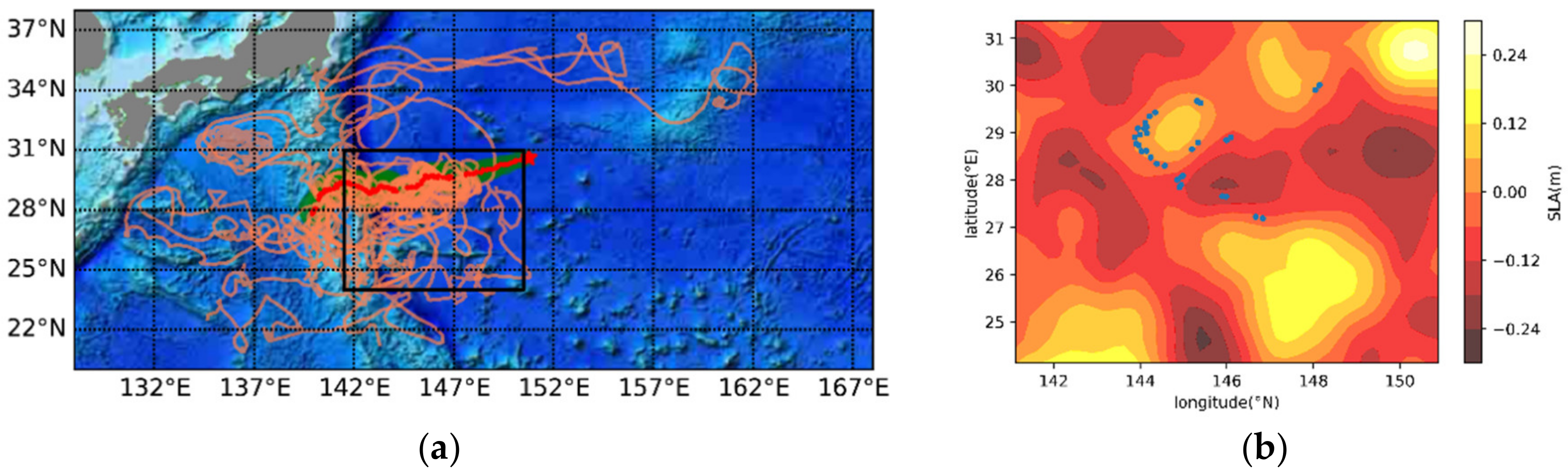
3.1. Distances between the Argo Positions and the Along-Track Positions
3.2. Barotropic Influence
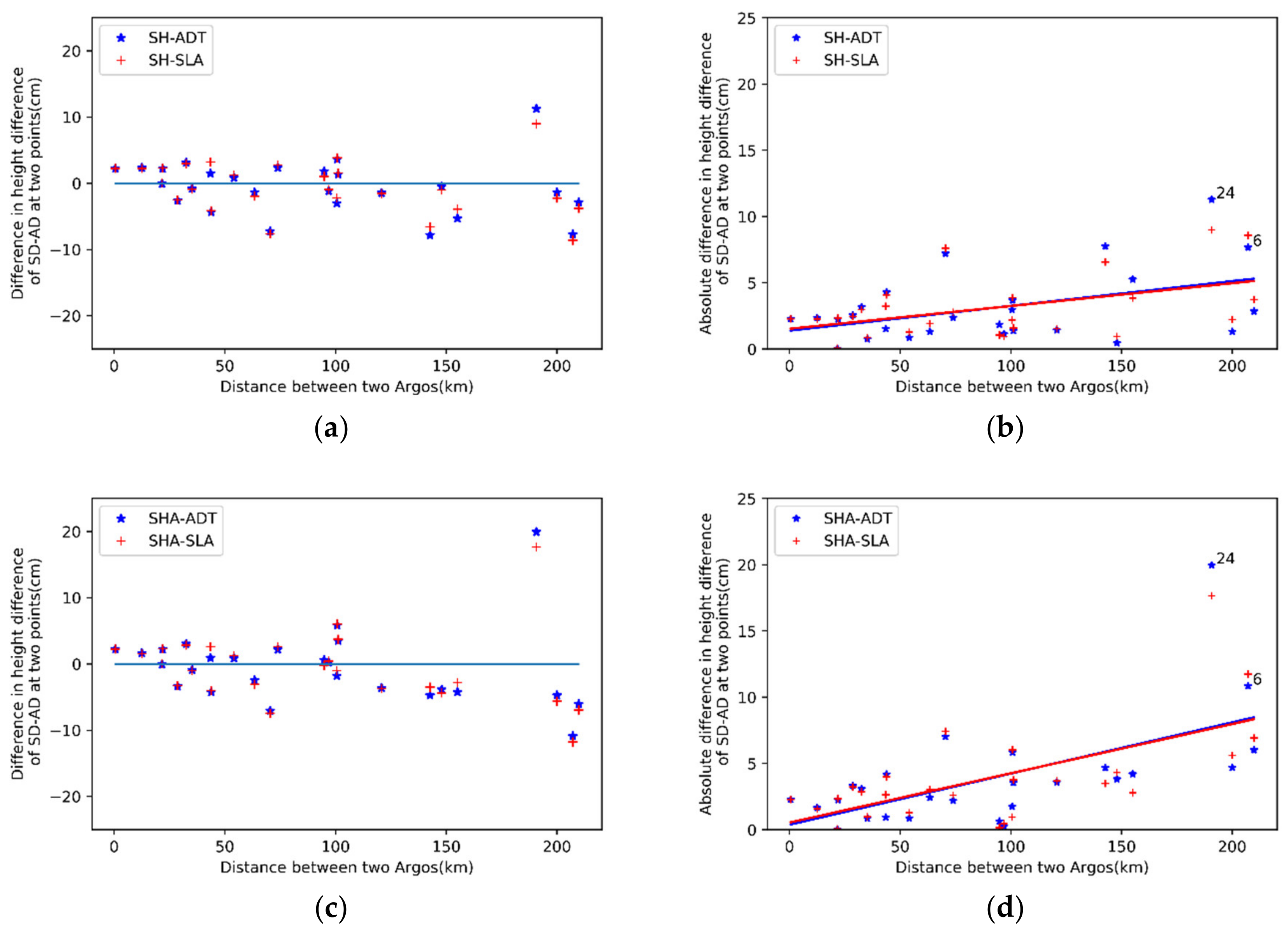
3.2.1. Distance between Two Points
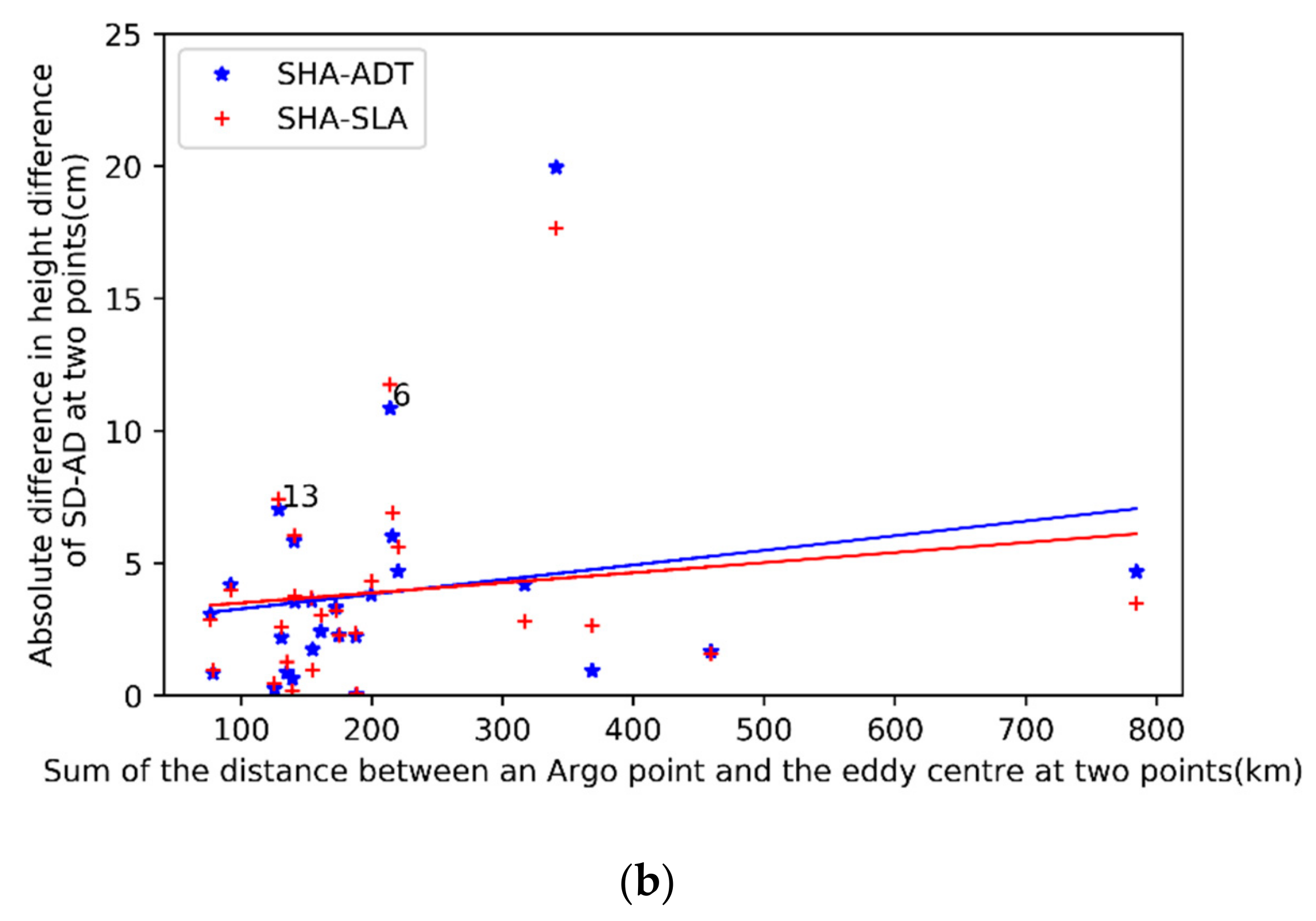
3.2.2. Distances between the Argo Points and the Eddy Centre
3.2.3. Wind Speeds
3.3. Results under the Conditions
4. Discussion
5. Conclusions
- The feasibility of validating the altimetry swath data by using the steric method. In this paper, we used in-situ observation data to analyze the feasibility of using a steric method to validate the interference altimetry sea level variability in different pixels. The result showed that when considering the distance difference between the distance of the Argo and the satellite in and and angle difference, the distance between two Argo points, the sum of the distance of the Argo point and the eddy center in and and the difference in wind speed between two Argo points, the relationship of the SD-AD has a highly corrected coefficient of 0.98, the RMSD was ~1.8 cm and the bias was ~0.6 cm. This proved that it is feasible to validate interferometric altimetry data using the steric method under these conditions.
- As we can see from Figure 4, Figure 5, Figure 6, Figure 7, Figure 8, Figure 9 and Figure 10, when the distance difference between the distance of the Argo and the satellite in and were less than ~13 km, and in the same direction, the distance between two Argo points was less than ~120 km, the sum of the distance of the Argo point and the eddy center in and less than 220 km, difference in wind speed between two Argo points were less than ~1 m/s and the non-steric influence had a significant reduction. The relationship between the steric data and sea level data had a highly corrected coefficient of 0.98. This proved that using the steric method to validate the sea level variability in different pixels is feasible, and the relationship needs to be studied in more detail in the future.
Author Contributions
Funding
Acknowledgments
Conflicts of Interest
Abbreviations
| ADT | Absolute Dynamic Topography |
| AE | Anticyclonic Eddy |
| AVISO | Archiving, Validation and Interpretation of Satellite Oceanographic |
| Cal/Val | Calibration and Validation |
| CMEMS | Copernicus Marine Environment Monitoring Service |
| ECMWF | European Centre for Medium Weather Forecasting |
| GDAC | Global Data Assembly Centers |
| IFREMER | French Research Institute for Exploitation of the Sea |
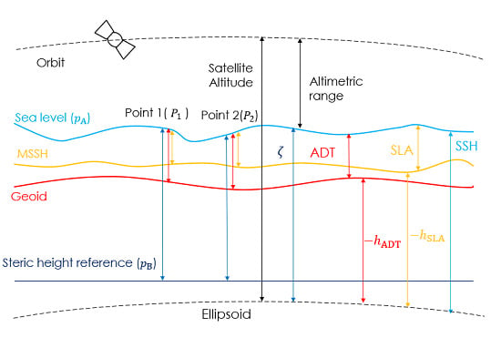
| MSSH | Mean Sea Surface Height |
| MSH | Mean Steric Height |
| NSH | Non-Steric Height |
| OW | Okubo–Weiss method |
| Point 1 | |
| Point 2 | |
| RMSD | Root Mean Square Deviation |
| SD-AD | Steric Data and Along-track Data |
| SH | Steric Height |
| SHA | Steric Height Anomaly |
| SLA | Sea Level Anomaly |
| SSH | Sea Surface Height |
| SWOT | Surface Water and Ocean Topography |
| T-S-P | Temperature-Salinity-Pressure |
| WOA 13 | World Ocean Atlas 2013 |
| 4D-Var | Four-Dimensional Variational Analysis |
References
- Johnson, D.R.; Thompson, J.D.; Hawkins, J.D. Circulation in the Gulf of Mexico from Geosat altimetry during 1985–1986. J. Geophys. Res. Ocean. 1992, 97, 2201. [Google Scholar] [CrossRef]
- Fu, L.-L.; Ubelmann, C. On the Transition from Profile Altimeter to Swath Altimeter for Observing Global Ocean Surface Topography. J. Atmos. Ocean. Technol. 2014, 31, 560–568. [Google Scholar] [CrossRef]
- Chen, G.; Tang, J.; Zhao, C.; Wu, S.; Yu, F.; Ma, C.; Xu, Y.; Chen, W.; Zhang, Y.; Liu, J.; et al. Concept Design of the “Guanlan” Science Mission: China’s Novel Contribution to Space Oceanography. Front. Mar. Sci. 2019, 6, 194. [Google Scholar] [CrossRef] [Green Version]
- Morrow, R.; Fu, L.-L.; Ardhuin, F.; Benkiran, M.; Chapron, B.; Cosme, E.; d’Ovidio, F.; Farrar, J.T.; Gille, S.T.; Lapeyre, G.; et al. Global Observations of Fine-Scale Ocean Surface Topography With the Surface Water and Ocean Topography (SWOT) Mission. Front. Mar. Sci. 2019, 6, 232. [Google Scholar] [CrossRef]
- Fu, L.L.; Ferrari, R. Observing Oceanic Submesoscale Processes From Space. Eos Trans. Am. Geophys. Union 2013, 89, 488. [Google Scholar] [CrossRef]
- Bonnefond, P.; Exertier, P.; Laurain, O.; Ménard, Y.; Orsoni, A.; Jan, G.; Jeansou, E. Absolute Calibration of Jason-1 and TOPEX/Poseidon Altimeters in Corsica Special Issue: Jason-1 Calibration/Validation. Mar. Geod. 2010, 26, 261–284. [Google Scholar] [CrossRef]
- Christensen, E.J.; Haines, B.J.; Keihm, S.J.; Morris, C.S.; Norman, R.A.; Purcell, G.H.; Williams, B.G.; Wilson, B.D.; Born, G.H.; Parke, M.E.; et al. Calibration of TOPEX/POSEIDON at Platform Harvest. J. Geophys. Res. 1994, 99, 24465. [Google Scholar] [CrossRef]
- Mertikas, S.P.; Daskalakis, A.; Tziavos, I.N.; Vergos, G.S.; Frantzis, X.; Tripolitsiotis, A.; Partsinevelos, P.; Andrikopoulos, D.; Zervakis, V. Ascending and Descending Passes for the Determination of the Altimeter Bias of Jason Satellites using the Gavdos Facility. Mar. Geod. 2011, 34, 261–276. [Google Scholar] [CrossRef]
- Watson, C.; Coleman, R.; White, N.; Church, J.; Govind, R. Absolute Calibration of TOPEX/Poseidon and Jason-1 Using GPS Buoys in Bass Strait, Australia Special Issue: Jason-1 Calibration/Validation. Mar. Geod. 2010, 26, 285–304. [Google Scholar] [CrossRef]
- Liu, Y.; Tang, J.; Zhu, J.; Lin, M.; Zhai, W.; Chen, C. An improved method of absolute calibration to satellite altimeter: A case study in the Yellow Sea, China. 2014, 33, 103–112. Acta Oceanol. Sinica 2014, 33, 103–112. [Google Scholar] [CrossRef]
- Jan, G.; Ménard, Y.; Faillot, M.; Lyard, F.; Jeansou, E.; Bonnefond, P. Offshore Absolute Calibration of Space-Borne Radar Altimeters. Mar. Geod. 2004, 27, 615–629. [Google Scholar] [CrossRef]
- Li, Z.; Wang, J.; Fu, L.L. An Observing System Simulation Experiment for Ocean State Estimation to Assess the Performance of the SWOT Mission: Part 1—A Twin Experiment. J. Geophys. Res. Ocean. 2019, 124, 4838–4855. [Google Scholar] [CrossRef]
- Wang, J.; Fu, L.-L.; Qiu, B.; Menemenlis, D.; Farrar, J.T.; Chao, Y.; Thompson, A.F.; Flexas, M.M. An Observing System Simulation Experiment for the Calibration and Validation of the Surface Water Ocean Topography Sea Surface Height Measurement Using In Situ Platforms. J. Atmos. Ocean. Technol. 2018, 35, 281–297. [Google Scholar] [CrossRef]
- Wahr, J.; Smeed, D.A.; Leuliette, E.; Swenson, S. Seasonal variability of the Red Sea, from satellite gravity, radar altimetry, and in situ observations. J. Geophys. Res. Ocean. 2015, 119, 5091–5104. [Google Scholar] [CrossRef] [Green Version]
- Guinehut, S.; Le Traon, P.-Y.; Larnicol, G. What can we learn from Global Altimetry/Hydrography comparisons? Geophys. Res. Lett. 2006, 33, 10. [Google Scholar] [CrossRef] [Green Version]
- Tapley, B.D.; Srinivas, B.; Ries, J.C.; Thompson, P.F.; Watkins, M.M. GRACE measurements of mass variability in the Earth system. Science 2004, 305, 503–505. [Google Scholar] [CrossRef] [Green Version]
- Roemmich, D.; Gilson, J.; Sutton, P.; Zilberman, N. Multidecadal Change of the South Pacific Gyre Circulation. J. Phys. Oceanogr. 2016, 46, 1871–1883. [Google Scholar] [CrossRef]
- Meyssignac, B.; Piecuch, C.G.; Merchant, C.J.; Racault, M.F.; Palanisamy, H.; Macintosh, C.; Sathyendranath, S.; Brewin, R. Causes of the Regional Variability in Observed Sea Level, Sea Surface Temperature and Ocean Colour Over the Period 1993–2011. In Integrative Study of the Mean Sea Level and Its Components; Springer: Cham, Germany, 2017; pp. 187–215. [Google Scholar]
- Dhomps, A.L.; Guinehut, S.; Traon, P.Y.L.; Larnicol, G. A global comparison of Argo and satellite altimetry observations. Ocean. Sci. 2011, 7, 175–183. [Google Scholar] [CrossRef] [Green Version]
- Perigaud, C. Influence of interannual rainfall anomalies on sea level variations in the tropical Indian Ocean. J. Geophys. Res. 2003, 108, C10. [Google Scholar] [CrossRef]
- Song, Y.T.; Qu, T. Multiple Satellite Missions Confirming the Theory of Seasonal Oceanic Variability in the Northern North Pacific. Mar. Geod. 2011, 34, 477–490. [Google Scholar] [CrossRef]
- Shao, Q.; Zhao, J. Comparing the steric height in the Nordic Seas with satellite altimeter sea surface height. Acta Oceanol. Sin. 2015, 34, 32–37. [Google Scholar] [CrossRef]
- Dandapat, S.; Chakraborty, A. Mesoscale Eddies in the Western Bay of Bengal as Observed From Satellite Altimetry in 1993–2014: Statistical Characteristics, Variability and Three-Dimensional Properties. IEEE J. Sel. Top. Appl. Earth Obs. Remote. Sens. 2016, 9, 5044–5054. [Google Scholar] [CrossRef]
- Henson, S.A.; Thomas, A.C. A census of oceanic anticyclonic eddies in the Gulf of Alaska. Deep. Sea Res. Part I 2008, 55, 163–176. [Google Scholar] [CrossRef]
- Xu, L.; Li, P.; Xie, S.P.; Liu, Q.; Liu, C.; Gao, W. Observing mesoscale eddy effects on mode-water subduction and transport in the North Pacific. Nat. Commun. 2016, 7, 10505. [Google Scholar] [CrossRef] [PubMed] [Green Version]
- Lázaro, C.; Juliano, M.F.; Fernandes, M.J. Semi-automatic determination of the Azores Current axis using satellite altimetry: Application to the study of the current variability during 1995–2006. Adv. Space Res. 2013, 51, 2155–2170. [Google Scholar]
- Rio, M.H. A mean dynamic topography computed over the world ocean from altimetry, in situ measurements, and a geoid model. J. Geophys. Res. 2004, 109, C12. [Google Scholar] [CrossRef] [Green Version]
- Baker-Yeboah, S.; Watts, D.R.; Byrne, D.A. Measurements of Sea Surface Height Variability in the Eastern South Atlantic from Pressure Sensor–Equipped Inverted Echo Sounders: Baroclinic and Barotropic Components. J. Atmos. Ocean. Technol. 2009, 26, 2593–2609. [Google Scholar] [CrossRef] [Green Version]
- Badin, G.; Williams, R.G.; Holt, J.T.; Fernand, L.J. Are mesoscale eddies in shelf seas formed by baroclinic instability of tidal fronts? J. Geophys. Res. Ocean. 2009, 114, C10. [Google Scholar] [CrossRef] [Green Version]
- Piecuch, C.G.; Calafat, F.M.; Dangendorf, S.; Jordà, G. The Ability of Barotropic Models to Simulate Historical Mean Sea Level Changes from Coastal Tide Gauge Data. Surv. Geophys. 2019, 40, 1399–1435. [Google Scholar] [CrossRef]
- Fourniotis, N.T.; Horsch, G.M. Three-dimensional numerical simulation of wind-induced barotropic circulation in the Gulf of Patras. Ocean. Eng. 2010, 37, 355–364. [Google Scholar] [CrossRef]
- Güting, P.M.; Hutter, K. Modeling wind-induced circulation in the homogeneous Lake Constance using. Aquat. Sci. 1998, 60, 266–277. [Google Scholar]
- Savage, A.C.; Arbic, B.K.; Richman, J.G.; Shriver, J.F.; Alford, M.H.; Buijsman, M.C.; Farrar, J.T.; Sharma, H.; Voet, G.; Wallcraft, A.J. Frequency content of sea surface height variability from internal gravity waves to mesoscale eddies. J. Geophys. Res. Ocean. 2017, 122, 2519–2538. [Google Scholar] [CrossRef]


| Control Condition | Root Mean Square Deviation (RMSD) | Bias | Correlation Coefficient | |||
|---|---|---|---|---|---|---|
| 0.2 degrees 4 hours | ADT | SLA | ADT | SLA | ADT | SLA |
| 5.25 cm | 4.42 cm | 1.54 cm | 1.18 cm | 0.8858 | 0.9034 | |
| 0.15 degrees 4 hours | ADT | SLA | ADT | SLA | ADT | SLA |
| 4.07 cm | 3.87 cm | 0.54 cm | 0.57 cm | 0.9241 | 0.9292 | |
| Control Condition | RMSD | BIAS | Correlation Coefficient | |||
|---|---|---|---|---|---|---|
| 0.2 degrees 4 hours | ADT | SLA | ADT | SLA | ADT | SLA |
| 7.79 cm | 6.56 cm | 2.46 cm | 2.09 cm | 0.7393 | 0.7994 | |
| 0.15 degrees 4 hours | ADT | SLA | ADT | SLA | ADT | SLA |
| 5.57 cm | 5.42 cm | 0.54 cm | 0.57 cm | 0.8862 | 0.8941 | |
| Argo Database | RMSD | BIAS | Correlation Coefficient | |||
|---|---|---|---|---|---|---|
| SH | ADT | SLA | ADT | SLA | ADT | SLA |
| 1.79 cm | 1.76 cm | 0.81 cm | 0.69 cm | 0.9785 | 0.9780 | |
| SHA | ADT | SLA | ADT | SLA | ADT | SLA |
| 1.76 cm | 1.89 cm | 0.66 cm | 0.55 cm | 0.9841 | 0.9828 | |
© 2020 by the authors. Licensee MDPI, Basel, Switzerland. This article is an open access article distributed under the terms and conditions of the Creative Commons Attribution (CC BY) license (http://creativecommons.org/licenses/by/4.0/).
Share and Cite
Zhang, Q.; Yu, F.; Chen, G. The Difference of Sea Level Variability by Steric Height and Altimetry in the North Pacific. Remote Sens. 2020, 12, 379. https://doi.org/10.3390/rs12030379
Zhang Q, Yu F, Chen G. The Difference of Sea Level Variability by Steric Height and Altimetry in the North Pacific. Remote Sensing. 2020; 12(3):379. https://doi.org/10.3390/rs12030379
Chicago/Turabian StyleZhang, Qianran, Fangjie Yu, and Ge Chen. 2020. "The Difference of Sea Level Variability by Steric Height and Altimetry in the North Pacific" Remote Sensing 12, no. 3: 379. https://doi.org/10.3390/rs12030379