Article

Elaborating Hungarian Segment of the Global Map of Salt-Affected Soils (GSSmap): National Contribution to an International Initiative

1
Institute for Soil Sciences and Agricultural Chemistry, Centre for Agricultural Research, H-1022 Budapest, Hungary
2
Department of Soil Science and Environmental Informatics, Georgikon Faculty, Szent István University, H-8360 Keszthely, Hungary
3
Lechner Knowledge Center, H-1149 Budapest, Hungary
*
Author to whom correspondence should be addressed.
Remote Sens. 2020, 12(24), 4073; https://doi.org/10.3390/rs12244073
Submission received: 8 November 2020 / Revised: 7 December 2020 / Accepted: 10 December 2020 / Published: 12 December 2020
(This article belongs to the Special Issue Global Gridded Soil Information Based on Machine Learning)

Abstract

:
Recently, the Global Map of Salt-affected Soils (GSSmap) was launched, which pursued a country-driven approach and aimed to update the global and country-level information on salt-affected soils (SAS). The aim of this paper was to present how Hungary contributed to GSSmap by preparing its own SAS maps using advanced digital soil mapping techniques. We used not just a combination of random forest and multivariate geostatistical techniques for predicting the spatial distribution of SAS indicators (i.e., pH, electrical conductivity and exchangeable sodium percentage) for the topsoil (0–30 cm) and subsoil (30–100 cm), but also a number of indices derived from Sentinel-2 satellite images as environmental covariates. The importance plots of random forests showed that in addition to climatic, geomorphometric parameters and legacy soil information, image indices were the most important covariates. The performance of spatial modelling was checked by 10-fold cross validation showing that the accuracy of the SAS maps was acceptable. By this study and by the resulting maps of it, we not just contributed to GSSmap, but also renewed the SAS mapping methodology in Hungary, where we paid special attention to modelling and quantifying the prediction uncertainty that had not been quantified or even taken into consideration earlier.

Graphical Abstract

1. Introduction

In the past decade, a number of international initiatives have been launched in order to provide thematic spatial soil information with relatively high resolution (from 1 km to 100 m) at the global scale, e.g., SoilGrids [1], Global Soil Map [2] and Global Soil Organic Carbon Map [3]. Nowadays, a country-driven (a.k.a “bottom-up”) approach is frequently pursued in which a given country is invited to prepare its own thematic soil maps for targeted soil properties and functions according to the specifications summarized in a guideline or “cookbook” (e.g., [3,4]). This approach has its own advantages and disadvantages, e.g., a map prepared by a country could be more accurate than a globally or continentally compiled one [5,6]. However, merging countrywide maps prepared by different countries (with possibly different methodology, sampling density, data quality etc.) are going to yield artefacts at state or country borders, which makes the final global map not so attractive [7,8].
Recently, an international initiative, namely Global Map of Salt-affected Soils (GSSmap), which has also pursued a country-driven approach, has been launched by the Global Soil Partnership (GSP) of the Food and Agriculture Organization (FAO). Salt-affected soils (SAS) are groups of soils with a high content of soluble salts and/or high amounts of sodium ions and have significant impacts on the environment, water and agriculture [4]. GSSmap is aimed at updating the global and country-level information on these soils and lay ground for future monitoring [4]. The initiative is highly appreciated because the global distribution of salt-affected soils was first estimated in the late 1970s by Szabolcs [9] and since then there has not been consistent updates of the global distribution [4]. In the framework of GSSmap, the role of the countries is to prepare and deliver their own SAS maps for the topsoil (0–30 cm) and for the subsoils (30–100 cm) with quantified prediction uncertainty, which calls for using advanced digital soil mapping techniques. The global map of GSSmap is expected to be published in December, 2020.
Digital soil mapping (DSM), which has become a successful sub-discipline of soil science with an active research output [10], aims to provide spatial soil information for a wide range of studies, such as precision agriculture [11,12], hydrology [13,14,15], environmental sciences [16,17], conservation biology [18,19] or spatial planning [20,21]. For this purpose, geostatistical techniques are widely used, which have been complemented by machine learning algorithms in the past decade. Nowadays, these advanced geostatistical and machine learning techniques, as well as their combinations, are in use for inferring the spatial variations of soil properties, functions and/or services [22,23,24,25]. In addition to the new techniques, the amount of environmental covariates used in DSM is continuously expanding mainly thanks to remote sensing. Although digital elevation models and their derivatives (e.g., slope, aspect and topographic wetness index) are proved to be useful covariates in DSM, remote sensing is able to provide a huge amount of information on land surface with a continuously increasing spatial, temporal and spectral resolution [26,27,28]. By the combination of certain bands of satellite images, such image indices (e.g., normalized difference vegetation index, salinity index and vegetation soil salinity index) can be gained, which provide specific information for the problem in hand. Thus, a lot of papers have addressed the issue of exploiting information acquired by remote sensing techniques in spatial modelling and inferencing (e.g., [29,30,31,32]).
In Hungary, there is a long tradition and history of studying salt-affected soils that is nicely demonstrated by a huge number of monographs dedicated to this topic (e.g., [9,33,34,35,36]). Most of the areas with SAS can be found in the Great Hungarian Plain that is an alluvial plain filled up with thick alluvial sediments on an ancient seabed. Later loess formation also took place here and the influence of shallow fluctuating, saline-sodic groundwater, as well as permanent or temporary waterlogging created the conditions of SAS formation. Sodium ions, being considered as the most important factor, either dissolved from the Tertiary Era deposits into groundwater [37] or concentrated during consecutive drying and wetting of infiltrated water [38]. Systematic mapping of salt-affected soils has a history of more than a hundred years in Hungary. The first medium-scale SAS map (1:75,000) was prepared in the late 1920s by Arany [39] and Magyar [40] presenting the status and vegetation of salt-affected soils, respectively. Sigmond [33] prepared the first ever quantitative map of soil salinity at the scale of 1:300,000. The first large-scale SAS map (1:10,000) was compiled by Szabolcs [41], who later also compiled SAS maps not just for Europe [42] but for the world [9] as well. The latter is important because it was the basis for assessing the global distribution of salt-affected soils [4].
The objective of our study was to present how Hungary contributed to the GSSmap international initiative by preparing its own maps of salt-affected soils according to the GSSmap specifications. For this purpose, we applied not just a combination of advanced machine learning algorithms and multivariate geostatistical techniques but also a number of image indices exploiting a huge amount of relevant information contained in remote sensing images. Our maps were prepared with a resolution of 100 m because we wanted to simultaneously update the available SAS maps for Hungary.

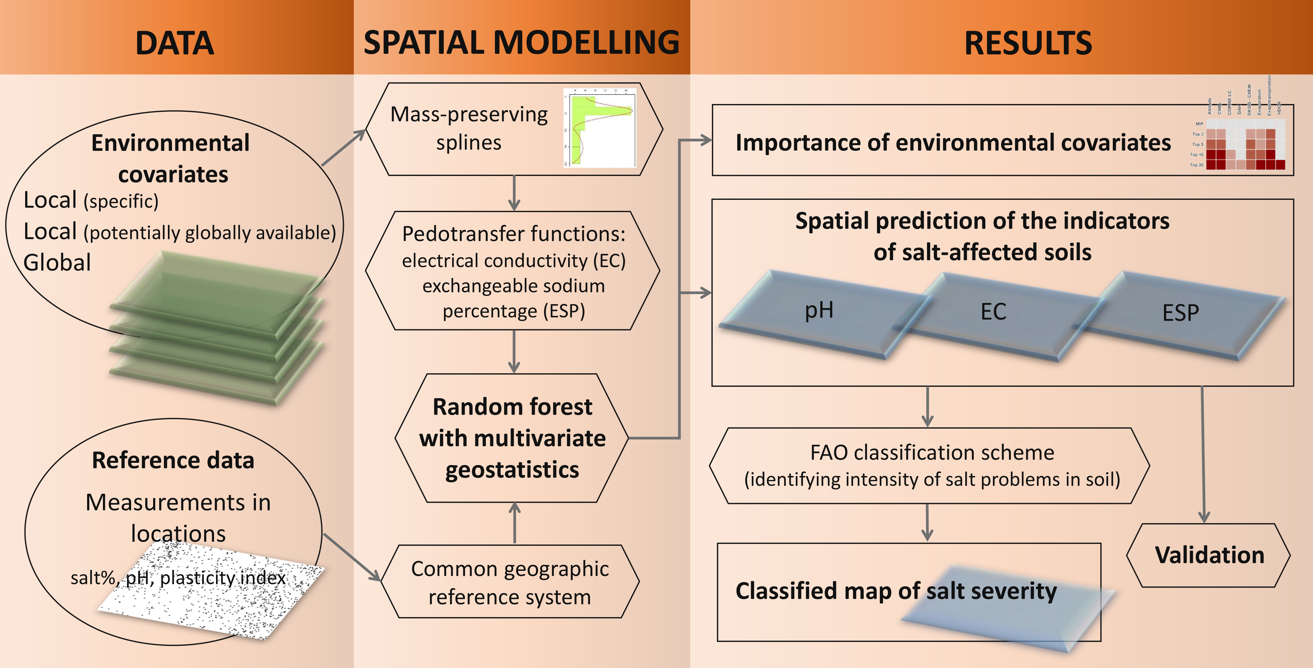
2. Materials and Methods

2.1. GSSmap Specifications

In the framework of GSSmap, three SAS indicators were selected, namely pH (H2O), electrical conductivity (EC) and exchangeable sodium percentage (ESP) of the soil paste extract, as identifiers of the status and occurrence of salt-affected soils. It was mandatory to map these indicators for the topsoil (0–30 cm) and for the subsoil (30–100 cm) with quantified prediction uncertainty that had to be expressed by the width of the 95% prediction interval. The target spatial resolution of the deliverable maps was 1 km. In addition to the maps of SAS indicators, it was also mandatory to prepare a classified salt severity map for the topsoil and for the subsoil with quantified prediction uncertainty using the maps of SAS indicators. Either the FAO or the USDA classification scheme could be used for preparing the map of salt severity. In summary, 4+4 maps for the topsoil and 4+4 maps for the subsoil were expected to be delivered by a country.

2.2. Soil Data, Conversion and Harmonization

For mapping the SAS indicators, we derived soil data from the Hungarian Soil Information and Monitoring System (SIMS) established in 1992 (Figure 1). SIMS is a countrywide monitoring system providing geographically referenced biological, physical and chemical information on the temporal change of the Hungarian soils. It consists of 4859 soil horizons belonging to 1236 soil profiles.
Since neither EC nor ESP of the soil paste-extract are part of the standard laboratory analysis of the soils in Hungary, thus neither does the laboratory protocol of SIMS extend to measure these indicators. For example, instead of measuring EC of the soil-paste extract, the measurement of salt concentration of the soil solution is preferred. Therefore, we had to use conversion methods in order to gain EC and ESP data. In Hungary, Filep [43], as well as Filep and Wafi [44] extensively studied the statistical relationships between EC, ESP and more commonly measured soil properties and elaborated a number of pedotransfer functions by adapting and modifying the internationally used functions. The main advantage of these pedotransfer functions is that they have been elaborated on a consistent and detailed data set of Hungarian SAS and therefore they have been specifically designed for deriving EC and ESP values for Hungarian salt-affected soils. Table 1 summarizes the pedotransfer functions used in this study.
Since the depth of soil horizons varies from one soil profile to another, we used mass-preserving splines [45] for modelling the vertical distribution of each SAS indicator at each soil profile. The fitted splines were used to derive the values of SAS indicators for the topsoil (0–30 cm) and for the subsoil (30–100 cm) at each monitoring point. The splined, so-called harmonized values of SAS indicators were used in further spatial modelling. Table 2 summarizes their descriptive statistics.

2.3. Environmental Covariates

Table 3 summarizes the environmental covariates used in spatial modelling. Representing the spatial variation of soil mantle, we used the genetic soil type map of Hungary [46] and a thematic layer of the Digital Kreybig Soil Information System (DKSIS [47]), namely the chemical properties of soils. The latter contains detailed, legacy, spatial information on the chemical properties of the Hungarian soils including categories of various types of SAS. Data layers provided by the Hungarian Meteorological Service were used to characterize climate. We characterized topography by a digital elevation model [48] and a number of its derivatives (see Table 3). Parent material was considered based on the correlation between the legend of the geological map of Hungary and 13 parent material classes according to the FAO code system [49].
In addition to the covariates summarized above, we also used a number of relevant indices derived from Sentinel-2 satellite images. The spectral bands of Sentinel-2 range from the visible and near infrared to the short wave infrared with a spatial resolution of 10, 20 and 60 m depending on the sensor. If the meteorological conditions are perfect, 22 Sentinel-2 satellite images in total are needed to cover Hungary entirely. However, due to cloudiness, 27 Sentinel-2 satellite images in total were used in this study, which were acquired during the spring of the year 2019 (i.e., 23/03/2019, 24/03/2019 and 31/03/2019). In the supplementary material, Figure S1 graphically presents the satellite images used in this study and their acquisition date. Spring is an appropriate period for surveying and mapping of salt-affected soils since soil mantle is either uncovered (i.e., bare) or only covered by natural vegetation. Using the satellite images, we compiled a countrywide, cloud-free mosaic for Hungary with the closest possible acquisition times. This mosaic was the basis for deriving satellite-based soil and/or vegetation indices. In this study, we derived those indices, which are the most frequently used in SAS mapping [4]. Table 4 presents these indices with their formulas. All the indices were computed at a resolution of 10 m in an automatized Python environment. Since SAS mapping was targeted with a resolution of 100 m, we aggregated the derived indices to 100 m using a median filter.
All the environmental covariates listed above were resampled into a common geographic reference system with a resolution of 100 m. This geographic reference system was also used in spatial modelling. In the case of categorical covariates (i.e., soil type, DKSIS chemical properties of soils, CORINE land cover, parent material), we applied a nearest neighbor resampling technique, whereas in the case of continuous covariates, a cubic spline technique was applied. Resampling was carried out in SAGA GIS software environment [51].

2.4. Spatial Modelling and Classification of SAS

The harmonized data on EC and ESP showed positively skewed distribution (Table 1) and therefore we applied log transformation in order to obtain quasi-normal distribution. The log-transformed EC and ESP data were used in further spatial modelling. The harmonized data on pH showed quasi-normal distribution.
Spatial variation of soil properties at a given depth can be described and modelled in terms of a deterministic component and a stochastic component, that is
Z d ( u ) = m d ( u ) + ε d ( u )
where Z is the soil property of interest, m is the deterministic component describing structural variation, ε is the stochastic part consisting of random variation that could be spatially correlated, u is the vector of the geographical coordinates, and d is the target soil depth. In this study, we used a combination of advanced machine learning algorithm and multivariate geostatistical techniques for modelling the spatial variation of the SAS indicators at both soil depths.
We used random forest (RF [52]) for describing, modelling and predicting the deterministic part of variation of the SAS indicators at both soil depths. We selected RF not only because it has become a frequently applied machine learning technique in various fields (e.g. [53,54,55,56]), but it commonly outperforms other techniques as well [23,57]. Before fitting RF between the indicators and the environmental covariates listed in Table 3, we fine-tuned the hyper-parameter mtry of RF that is the number of input covariates selected randomly at each split. A tuning vector was generated containing the possible values of mtry, and then a repeated 10-fold cross-validation was used for evaluating the performance on each SAS indicator at both soil depths. The fine-tuned values of mtry were used for fitting RF to each indicator and then the fitted RFs were used for spatially exhaustively predicting each SAS indicator at both soil depths.
Since we could reasonably assume that the SAS indicators are interdependent, it is better to jointly model their spatial variation at a given soil depth. Therefore, a geostatistical model, namely cokriging with external drift (coKED), was built up for each soil depth. In coKED, we used the RF predictions of the SAS indicators as external drifts, i.e., they were interpreted as deterministic, known functions of the SAS indicators (i.e., m ( u ) of Eq. 1). The residuals (i.e., the difference between the RF predictions and the observations of the SAS indicators) represented the stochastic part of variation of the SAS indicators (i.e., ε ( u ) of Eq. 1). We computed the direct- and cross-variograms of the residuals and then a linear model of coregionalization (LMC) was fitted in order to obtain a statistically valid model [58]. The spatial prediction of SAS indicators and their uncertainty were identified by the corresponding coKED prediction and its kriging variance, respectively. In the case of EC and ESP, we had to transform the coKED predictions back to the original, positively skewed scale since spatial modelling was carried out on a transformed, normal scale. It can be done by adding half of the kriging variance to the coKED prediction and then taking its exponential [59].
According to the GSSmap specifications, we finally classified the spatial predictions of the SAS indicators in order to prepare a salt severity map for both soil depths. For this purpose, we used the FAO classification scheme presented in Table 5.

2.5. Quantification and Propagation of Uncertainty

The prediction uncertainty of the SAS indicators was quantified by the width of the 95% prediction interval (PI). This PI reports the range of values within which the true value is expected to occur 95 times out of 100. If the distribution is normal, as in the case of pH, the upper and lower limit of the 95% PI can be readily computed by subtracting and adding 1.96 times the kriging standard deviation to the kriging prediction [60]. If the distribution is lognormal, as in the case of EC and ESP, the limits of the 95% PI are computed on the transformed, normal scale as above and then transformed back to the original, lognormal scale by taking their exponential [61]. The width of the 95% PI (i.e., the difference between the upper and lower limit) is a useful measure of uncertainty because its value can be interpreted as the higher the value, the higher the uncertainty [62].
We also examined how the prediction uncertainty of SAS indicators propagates through the classification scheme (Table 5) at both soil depths. Sequential Gaussian cosimulation was conducted to the geostatistical models built up in the section above and 100 equally probable stochastic realizations of the SAS indicators were simulated for both soil depths. Cosimulation was conditional, that is, it honored the SAS data at the monitoring locations. In addition, the generated stochastic realizations reproduced the joint spatial relationship (i.e., interdependency) of the SAS indicators. We used the generated 100 realizations as inputs of classification for investigating how the prediction uncertainty of inputs propagates through [63]. Thus, 100 classified salt severity maps were obtained for both soil depths, which means 100 simulated salt severity classes at each location for both soil depths. To quantify the uncertainty in the classification output, we used Shannon’s [64] information entropy, that is
H ( u ) = i = 1 N p i ( u ) · log p i ( u ) log N
where H ( u ) is the value of Shannon’s information entropy at location u , p i ( u ) is the probability of the ith salt severity class at location u , and N is the number of possible salt severity classes. The value of p i ( u ) was determined by the relative frequency of the ith salt severity class based on the 100 salt severity classes simulated at location u . Term in the denominator of Equation (2) ensures that the value of Shannon’s entropy falls within the interval [0,1]. Its value can be interpreted as the higher the value, the higher the uncertainty. If H ( u ) takes the value of zero, then there is no uncertainty, i.e., the probability of one of the possible classes is equal to one at location u . If H ( u ) takes the value of one, the uncertainty is highest, i.e., each possible class has equal probability of occurring at location u .

2.6. Validation

Due to the limited number of soil observations, we used 10-fold cross-validation for inspecting the performance of the spatial predictions and uncertainty quantifications of SAS indicators. In 10-fold cross-validation, the dataset is randomly partitioned into 10 equal-size parts. One of these parts is retained for validating the spatial predictions, which were given by using the remaining nine parts. This step is repeated until each of the 10 parts become a validation set exactly once.
We computed the most commonly used error measures, i.e., bias (mean error, ME) and the spread of the error distribution (root mean square error, RMSE). Furthermore, Lin’s [65] concordance correlation coefficient (CCC) and Nash-Sutcliffe [66] model efficiency coefficient (NSE) were computed.
We examined the performance of the uncertainty quantifications by using accuracy plots and G statistics. The underlying theory is that if an uncertainty quantification reports, e.g., the map of the 95% PI, then we expect that 95% of the observed values coming from the validation set should fall within this PI. If the observed fraction is lower than the expected fraction, then the uncertainty has been underestimated. If the observed fraction is higher, the uncertainty has been too liberally estimated (i.e., overestimated). This can be extended to any symmetric PIs. An accuracy plot (a.k.a. prediction interval coverage probability plot) graphically presents the expected and observed fraction for any symmetric PIs and ideally follows the 1:1 line. Based on the accuracy plot, G statistics [67] measures the overall closeness of the observed and the expected fractions, that is
G = 1 0 1 [ ξ ¯ ( p ) p ] d p
where ξ ¯ ( p ) and p are the observed and expected fraction for a p -width symmetric PI, respectively. The value of G statistics can be interpreted as the higher the value, the closer the observed and the expected fractions. Ideally, its value is equal to 1.

3. Results

3.1. Spatial Prediction of SAS Indicators

The log-transformed data on EC and ESP showed quasi normal distribution in both soil depths and therefore they could be easily conducted to spatial modelling. For pH, EC and ESP, mtry values of 9, 18 and 7 were found to be optimal in the topsoil, respectively, whereas mtry values of 14, 15 and 11 were found to be optimal in the subsoil for pH, EC and ESP, respectively.
The importance of the environmental covariates for each SAS indicators at both soil depths is given in the supplementary material (see Figure S2). A terser summary is given in Figure 2 in which the importance of a given environmental covariate was presented by counting its occurrence on the list of the top 3, 5, 10, and 20 important covariates of each SAS indicator. Besides, Figure 2 also presents the most important predictors (MIPs) for the SAS indicators, i.e., those ones which proved to be the most important (or best) covariates in predicting SAS indicators. Temperature, precipitation and evapotranspiration were found to be MIPs at both soil depths, which is not a surprise considering that salt-affected soils have developed with an excess of evaporation over precipitation, helping to raise salt from shallow groundwater [68]. In addition to the climatic data layers detailed above, DEM derivatives (i.e., altitude and channel network base level) and soil information (i.e., soil type and DKSIS’s chemical properties of soils) were found to be very important in predicting SAS indicators in the topsoil and subsoil based on the top three lists. Hungary is located in the Carpathian (or Pannonian) Basin, and thus, Hungarian salt-affected soils have been mainly formed in the Great Hungarian Plain, which are discharge areas of regional flow systems of groundwater characterized by surplus salts and especially sodium ions. The importance of DKSIS’s thematic layer of chemical properties of soils is evident in Figure 2, meaning that legacy spatial soil information provided by DKSIS are definitely valuable for predicting SAS indicators. Based on the top 5, 10 and 20 lists, we found that further DEM derivatives (e.g., vertical and horizontal distance to channel network, topographic wetness index), land cover and image indices (e.g., salinity index and ratio, brightness index and vegetation soil salinity index) derived from Sentinel-2 satellite images were also important in predicting SAS indicators at both soil depths. Image indices mainly represented the mosaic-like patches of salt-affected soils, which could be hardly captured by other covariates.
Figure 3 presents the experimental direct- and cross-variograms computed from the RFs residuals, and it also depicts the fitted LMCs at both soil depths. In both cases, LMCs have a nested model structure in which the first structure models the discontinuity at the origin (a.k.a. nugget effect), whereas the second one models spatial continuity with range values of 40 and 35 km in the topsoil and in the subsoil, respectively. The model type of the second structure was spherical at both soil depths.
Figure 4 presents the maps of the SAS indicators, whereas their prediction uncertainty is presented in the supplementary material (Figure S3). The spatial predictions represent well the overall spatial distribution of the SAS indicators in Hungary. High values of EC, ESP and pH have been predicted on those areas where it is well-known that soils are strongly affected by salinity, sodicity and/or alkalinity. These areas are mainly located in the Danube-Tisza Interfluve, the upper part of Tisza River and in the eastern part of Hungary. In addition, the maps presented in Figure 4 give a fairly detailed picture about the spatial variability of the SAS indicators, which makes it easy to identify the mosaic-like patches of salt-affected soils. We should note that the prediction uncertainty of ESP and EC was explicitly high on those areas, where the prediction of EC and ESP was also high. This is because both SAS indicators are lognormally distributed. A property of a lognormally distributed random variable is the proportional effect, i.e., variability is higher in areas with high average values than in areas with low average values [61]. This implies high prediction uncertainty in areas with high predicted values [62,69].

3.2. Performance of Spatial Predictions and Uncertainty Quantifications

In Table 6, we summarized the performance of the spatial predictions by the computed values of ME, RMSE, CCC and NSE. An important aim of every DSM procedure is to provide predictive soil maps without bias (i.e., value of ME close to zero) and with RMSE as low as possible. According to the error measures, the spatial models gave unbiased spatial predictions for each SAS indicator at both soil depths. The values of CCC range from 0.531 to 0.764. The values of NSE can be interpreted as the value of R-square if its value is greater than zero. The values of NSE range from 0.333 to 0.621. The lowest values were obtained for ESP, meaning that its performance was the lowest between the SAS indicators.
We also checked the performance of the uncertainty quantifications of the SAS indicators by accuracy plots and G statistics. Figure 5 presents the prepared accuracy plots and computed G statistics for each SAS indicator at both soil depths. The accuracy plots approximately follow the 1:1 line, proving that the accuracy of uncertainty quantifications is acceptable. This statement is also supported by the computed G statistics, which are quite close to the expected value.

3.3. Classified Maps of Salt Severity

Figure 6 presents the classified salt severity maps for the topsoil and for the subsoil. Areas with already known salt-affected soils are well reflected in the classified maps, if we compare them with Szabolcs’s [42] map (see Figure S4). However, the comparison of these maps is not so straightforward since the SAS categories presented in Szabolcs’s map were defined according to the Hungarian soil classification system, which distinguishes salt-affected soils by (i) the vertical distribution of salinity, sodicity and alkalinity; (ii) the soil structure; and (iii) the vertical sequence of diagnostic horizons [70]. Nonetheless, areas severely affected by salinity or sodicity are quite similar in Szabolcs’s map and in the classified salt severity maps. These areas are mainly located in the Danube-Tisza Interfluve, upper part of Tisza River and in the eastern part of Hungary. Though the improvement (i.e., reclamation or amelioration) of these soils is scientifically well founded in Hungary, it is a rather costly operation. This is the reason why large parts of these areas are kept as graze-land or hayfield, land for afforestation, paddy field, or fishpond. Besides, most of the Hungarian National Parks have salt-affected grasslands, hayfields, marshes, reed-lands, and lakes, and these provide habitat for protected animals (mainly birds), plants and attract lots of tourists.
It should be mentioned that the FAO classification scheme (Table 5) proposed by the GSSmap specification is not so appropriate for classifying Hungarian salt-affected soils since it applies a very strict threshold on salinity (i.e., 0.75 dS·m−1). Furthermore, the threshold on sodicity is not so strict with the common ESP value of 15% (Table 5). That is the reason why areas of slight and moderate salinity classes, as well as areas of slight sodicity class, are so widespread in Hungary, especially in the eastern part of Hungary and in the Danube-Tisza Interfluve (Figure 6). This can be attributed to the fact that large parts of the Hungarian lowlands have been affected by stagnant water and consequently have fine sediments with some minor soluble salt concentration. Since the values of EC reflect not only soluble salts but also fine particles and organic matter [71], the categories of slight and moderate salinity also reflect clayey soils, which are quite widespread in the eastern part of Hungary. These areas are classified as “potential salt-affected soils” in Szabolcs’s map (see Figure S4), meaning that these areas could be potentially threated by salt problems.
The quantified uncertainty in the SAS classification outputs is presented in the supplementary material (see Figure S5). There is a strong relationship between the uncertainty in SAS classification outputs and the prediction uncertainty of the SAS indicators (Figure S3), i.e., the higher the prediction uncertainty of SAS indicators, the higher the uncertainty in the SAS classification output. This is quite conspicuous for salinity (i.e., EC) and sodicity (i.e., ESP). This could be attributed to the fact that the prediction uncertainty of ESP and EC was explicitly high on those areas, where the prediction of ESP and EC was also high. This is why areas strongly affected by salinity or sodicity show higher uncertainty in the SAS classification than areas without salt problems.

4. Discussion

This section was addressed to discuss some issues in more detail in relation to the methodology and environmental covariates used in this study. Two of them were raised in the course of spatial modelling, whereas one of them relates to the remote sensing images applied as environmental covariates.

4.1. On the Interpretability of Machine Learning Algorithms

It is commonly known that data-driven models given by machine learning algorithms (MLAs), including RF, are not easily interpretable since they are too complex and complicated to understand. They frequently appear like a black box in which it is hard to trace and understand what happens. Although there are some MLAs, which can provide more-or-less easily interpretable models (e.g., cubist), the most of them cannot do so. Prediction accuracy and model interpretability are in conflict as it was pointed out by Breiman [72]. Thus, in most cases, a more accurate prediction can be gained by a complex and complicated model than by a simple and easily interpretable one. However, we should try to understand these models as far as possible [73], e.g., by the application of post-hoc techniques [74,75]. The importance plot derived from a RF model can be a valuable tool trying to do so. In this study, we examined these plots of the environmental covariates (Figure S2) at different levels of importance (Figure 2) and tried to interpret with expert knowledge why these environmental covariates were important in predicting SAS indicators in Hungary. Obviously, it did not give a full picture about the fitted RFs but, at least, there was a chance to explore and try to interpret the main relationships between the SAS indicators and the environmental covariates, which defined these predictive models. We could identify the background, conditions and driving forces of SAS formation, which is important for studying, mapping and monitoring of these soils.

4.2. Remotely Sensed Information as Important Covariates for SAS Mapping

Remotely sensed information, including aerial photographs, on land surface have been used for decades to study the spatio-temporal variability of salt-affected soils (e.g., [29,30,76,77]). Thus, we dedicated a separate subsection to discuss and highlight the importance of remote sensing in SAS mapping. In this study, we pointed out that indices derived from remotely sensed images were informative covariates (Figure S2 and Figure 2) in representing smaller scale spatial variability of salt-affected soils. Indeed, conditions and driving forces of SAS formation operate at various scales and, therefore, it is a real challenge to map these soils accurately. We have seen that environmental covariates associated with topography and climate were principal because they are important conditions and driving forces of the potential occurrence of SAS at a larger scale. However, salt-affected soils frequently appear as mosaic-like patches. This can be attributed to conditions and driving forces operating at a much smaller scale, such as microtopography or microclimate, which can be hardly taken into consideration directly, especially when countrywide SAS mapping is targeted. The easiest way to capture this small scale variability is the application of image indices derived from remotely sensed information. Indices can provide specific, spatially (or even spatio-temporally) detailed information on the mosaic-like appearance of SAS via the natural vegetation or bare soil surface. It is commonly known that halophytes (i.e., salt-tolerant plants) and their communities are important indicators of SAS and are closely related to mosaic-like patches of SAS. This knowledge on botanic and ecology have been used for decades in field surveying and mapping of SAS [78,79]. Indices derived from remotely sensed images are able to provide information on the occurrence of these plant communities and, therefore, these indices as environmental covariates can be successfully used for modelling smaller scale spatial variability of SAS. Furthermore, since these plant communities are differentiated by microtopography [78], indices containing information on these plant communities can also provide indirect information on the characteristic of microtopography, which cannot be reflected by a countrywide digital elevation model with a relatively low resolution.

4.3. Pros And Cons of Using Multivariate Geostatistics

In this study, we used multivariate geostatistics, to be more precise the cokriging approach, with random forest since we could reasonably assume that the SAS indicators are interdependent and jointly vary in space. The computed experimental direct- and cross-variograms (Figure 3) confirmed this assumption and, therefore, we jointly modelled the spatial distribution of SAS indicators, which is a rarely used approach in practice. When two or more variables are targeted for mapping or spatial modelling, it is common in practice to model their spatial distribution separately. In geostatistics, Goovaerts [58], Wackernagel [80] and Cressie [81] pointed out that this approach could yield inconsistent results, e.g., the sum of the separately kriged particle size fractions of the soils (i.e., sand, silt and clay) is not going to be 100%. Therefore, it is better to jointly model their spatial distribution. The application of the cokriging approach is able not just to exploit the advantages of this interdependency in spatial modelling but also to provide consistent results that are highly appreciated in further assessment [58,80,81]. Besides, in this study, this approach allowed us to generate such stochastic realizations that honored the joint spatial distribution of the SAS indicators and to examine in a consistent way (thanks to these realizations) how the prediction uncertainty of the SAS indicators propagates through the SAS classification scheme. As a matter of fact, there are some disadvantages that make the cokriging approach not so attractive in practice. In this study, we modelled the spatial distribution of three SAS indicators, which meant three direct- and three cross-variograms for a given soil depth (Figure 3), and then we used a linear model of coregionalization (Figure 3) to fit a statistically valid model. As the number of variables increases, not just the number of direct- and cross-variograms increases exponentially, which have to be modelled, but also the modelling becomes complicated and needs more effort because of the increasing number of conditions that have to be satisfied (for more details see Goovaerts [58]).

5. Conclusions

The objective of our paper was to present how Hungary contributed to GSSmap by preparing its own SAS maps using advanced DSM techniques. We used a combination of random forest and multivariate geostatistics for jointly modelling and predicting the spatial distribution of the selected SAS indicators with special attention to quantifying the prediction uncertainty and how this uncertainty propagates through the SAS classification scheme recommended by FAO.
By the interpretation of the importance plots of the fitted RFs, we have explored and identified the conditions and driving forces of SAS formation at various scales, which could support further studies on SAS. Furthermore, these findings can serve as a basis not just for better understanding the spatial distribution of SAS but also for further surveying, mapping and monitoring of these soils.
In this study, we have pointed out that indices derived from remotely sensed images can serve as highly informative covariates in digital mapping of salt-affected soils. It was revealed that short-scale variability of salt-affected soils, which causes mosaic-like patches in field, can be appropriately captured and modelled via remote sensing indices.
As we have highlighted, there is a long history and tradition of studying salt-affected soils in Hungary, and there are a number of SAS maps with varying scales. By this study and by the resulting maps of it, we not just successfully contributed to the GSSmap international initiative and complemented the available map series of salt-affected soils in Hungary, but also renewed their mapping methodology by using advanced DSM techniques. In the renewal of the methodology, we paid special attention to modelling and quantifying the prediction uncertainty that had not been quantified or even taken into consideration earlier.

Supplementary Materials

The following are available online at https://www.mdpi.com/2072-4292/12/24/4073/s1, Figure S1: Sentinel-2 satellite images and their acquisition date, Figure S2: Importance of environmental covariates, Figure S3: Prediction uncertainty of the indicators of salt-affected soils, Figure S4: Map of salt-affected soils compiled by Szabolcs (1974), and Figure S5: Propagation of uncertainty in classification of salt-affected soils.

Author Contributions

Conceptualization, G.S., Z.B. and L.P.; methodology, G.S. and L.P.; software, G.S.; validation, G.S., Z.B., A.L., T.T. and L.P.; formal analysis, G.S. and Z.B.; investigation, Z.B., A.L., R.P. and O.P.; data curation, A.L., R.P. and O.P.; writing—original draft preparation, G.S., Z.B., A.L., T.T. and L.P.; writing—review and editing, G.S., Z.B., T.T. and A.L.; visualization, G.S. and A.L.; supervision, Z.B., and L.P.; project administration, G.S.; funding acquisition, G.S., T.T. and L.P. All authors have read and agreed to the published version of the manuscript.

Funding

This research was funded by the National Research, Development and Innovation Office (NKFIH), grant numbers K-131820 and K-124290. The work of G.S. was supported by the Premium Postdoctoral Scholarship of the Hungarian Academy of Sciences. The APC was funded by the Premium Postdoctoral Scholarship of the Hungarian Academy of Sciences.

Acknowledgments

The authors thank J. Matus and B. Bártfai for their indispensable contributions.

Conflicts of Interest

The authors declare no conflict of interest.

References

  1. Hengl, T.; Mendes de Jesus, J.; Heuvelink, G.B.M.; Ruiperez Gonzalez, M.; Kilibarda, M.; Blagotić, A.; Shangguan, W.; Wright, M.N.; Geng, X.; Bauer-Marschallinger, B.; et al. SoilGrids250m: Global gridded soil information based on machine learning. PLoS ONE 2017, 12, e0169748. [Google Scholar] [CrossRef] [PubMed] [Green Version]
  2. Arrouays, D.; Grundy, M.G.; Hartemink, A.E.; Hempel, J.W.; Heuvelink, G.B.M.; Hong, S.Y.; Lagacherie, P.; Lelyk, G.; McBratney, A.B.; McKenzie, N.J.; et al. GlobalSoilMap. Toward a Fine-Resolution Global Grid of Soil Properties. Adv. Agron. 2014, 125, 93–134. [Google Scholar] [CrossRef]
  3. Yigini, Y.; Olmedo, G.F.; Reiter, S.; Baritz, R.; Viatkin, K.; Vargas, R. Soil Organic Carbon Mapping Cookbook, 2nd ed.; FAO: Rome, Italy, 2018. [Google Scholar]
  4. Omuto, C.T.; Vargas, R.R.; El Mobarak, A.M.; Mohamed, N.; Viatkin, K.; Yigini, Y. Mapping of Salt-Affected Soils: Technical Manual; FAO: Rome, Italy, 2020. [Google Scholar]
  5. Vitharana, U.W.A.; Mishra, U.; Mapa, R.B. National soil organic carbon estimates can improve global estimates. Geoderma 2019, 337, 55–64. [Google Scholar] [CrossRef]
  6. Szatmári, G.; Pirkó, B.; Koós, S.; Laborczi, A.; Bakacsi, Z.; Szabó, J.; Pásztor, L. Spatio-temporal assessment of topsoil organic carbon stock change in Hungary. Soil Tillage Res. 2019, 195, 104410. [Google Scholar] [CrossRef]
  7. Heuvelink, G.B.M. It’s the accuracy. Pedometron 2015, 37, 14–16. [Google Scholar]
  8. Hengl, T. On usability of soil maps (and on global soil data models vs stitching together of individual disparate soil maps). Pedometron 2015, 38, 19–24. [Google Scholar]
  9. Szabolcs, I. Review of Research on Salt Affected Soils. Natural Resources Research; UNESCO: Paris, France, 1979. [Google Scholar]
  10. Minasny, B.; McBratney, A.B. Digital soil mapping: A brief history and some lessons. Geoderma 2016, 264, 301–311. [Google Scholar] [CrossRef]
  11. Söderström, M.; Sohlenius, G.; Rodhe, L.; Piikki, K. Adaptation of regional digital soil mapping for precision agriculture. Precis. Agric. 2016, 17, 588–607. [Google Scholar] [CrossRef] [Green Version]
  12. Piikki, K.; Wetterlind, J.; Söderström, M.; Stenberg, B. Three-dimensional digital soil mapping of agricultural fields by integration of multiple proximal sensor data obtained from different sensing methods. Precis. Agric. 2014, 16, 29–45. [Google Scholar] [CrossRef]
  13. Decsi, B.; Vári, Á.; Kozma, Z. The effect of future land use changes on hydrologic ecosystem services: A case study from the Zala catchment, Hungary. Biol. Futur. 2020, 1, 3. [Google Scholar] [CrossRef]
  14. Decsi, B.; Ács, T.; Kozma, Z. Long-term Water Regime Studies of a Degraded Floating Fen in Hungary. Period. Polytech. Civ. Eng. 2020, 64, 951–963. [Google Scholar] [CrossRef]
  15. Jolánkai, Z.; Kardos, M.K.; Clement, A. Modification of the MONERIS Nutrient Emission Model for a Lowland Country (Hungary) to Support River Basin Management Planning in the Danube River Basin. Water 2020, 12, 859. [Google Scholar] [CrossRef] [Green Version]
  16. Tóth, G.; Hermann, T.; Szatmári, G.; Pásztor, L. Maps of heavy metals in the soils of the European Union and proposed priority areas for detailed assessment. Sci. Total Environ. 2016, 565, 1054–1062. [Google Scholar] [CrossRef] [PubMed]
  17. Pásztor, L.; Szabó, K.Z.; Szatmári, G.; Laborczi, A.; Horváth, Á. Mapping geogenic radon potential by regression kriging. Sci. Total Environ. 2016, 544, 883–891. [Google Scholar] [CrossRef] [PubMed]
  18. Szilassi, P.; Szatmári, G.; Pásztor, L.; Árvai, M.; Szatmári, J.; Szitár, K.; Papp, L. Understanding the Environmental Background of an Invasive Plant Species (Asclepias syriaca) for the Future: An Application of LUCAS Field Photographs and Machine Learning Algorithm Methods. Plants 2019, 8, 593. [Google Scholar] [CrossRef] [PubMed] [Green Version]
  19. Tanács, E.; Belényesi, M.; Lehoczki, R.; Pataki, R.; Petrik, O.; Standovár, T.; Pásztor, L.; Laborczi, A.; Szatmári, G.; Molnár, Z.; et al. Országos, nagyfelbontású ökoszisztéma- alaptérkép: Módszertan, validáció és felhasználási lehetőségek. Természetvédelmi Közlemények 2019, 25, 34–58. [Google Scholar] [CrossRef]
  20. Laborczi, A.; Bozán, C.; Körösparti, J.; Szatmári, G.; Kajári, B.; Túri, N.; Kerezsi, G.; Pásztor, L. Application of Hybrid Prediction Methods in Spatial Assessment of Inland Excess Water Hazard. ISPRS Int. J. Geo-Inf. 2020, 9, 268. [Google Scholar] [CrossRef]
  21. Pásztor, L.; Laborczi, A.; Takács, K.; Szatmári, G.; Fodor, N.; Illés, G.; Farkas-Iványi, K.; Bakacsi, Z.; Szabó, J. Compilation of Functional Soil Maps for the Support of Spatial Planning and Land Management in Hungary. In Soil Mapping and Process Modeling for Sustainable Land Use Management; Pereira, P., Brevik, E.C., Munoz-Rojas, M., Miller, B.A., Eds.; Elsevier Ltd.: Amsterdam, The Nethelands, 2017; pp. 293–317. [Google Scholar]
  22. Veronesi, F.; Schillaci, C. Comparison between geostatistical and machine learning models as predictors of topsoil organic carbon with a focus on local uncertainty estimation. Ecol. Indic. 2019, 101, 1032–1044. [Google Scholar] [CrossRef]
  23. Nussbaum, M.; Spiess, K.; Baltensweiler, A.; Grob, U.; Keller, A.; Greiner, L.; Schaepman, M.E.; Papritz, A. Evaluation of digital soil mapping approaches with large sets of environmental covariates. Soil Discuss. 2017, 1–32. [Google Scholar] [CrossRef] [Green Version]
  24. Szabó, B.; Szatmári, G.; Takács, K.; Laborczi, A.; Makó, A.; Rajkai, K.; Pásztor, L. Mapping soil hydraulic properties using random-forest-based pedotransfer functions and geostatistics. Hydrol. Earth Syst. Sci. 2019, 23, 2615–2635. [Google Scholar] [CrossRef] [Green Version]
  25. Keskin, H.; Grunwald, S. Regression kriging as a workhorse in the digital soil mapper’s toolbox. Geoderma 2018, 326, 22–41. [Google Scholar] [CrossRef]
  26. Mulder, V.L.; de Bruin, S.; Schaepman, M.E.; Mayr, T.R. The use of remote sensing in soil and terrain mapping—A review. Geoderma 2011, 162, 1–19. [Google Scholar] [CrossRef]
  27. Dwivedi, R.S. Remote Sensing of Soils; Springer: Berlin/Heidelberg, Germany, 2017; ISBN 9783662537404. [Google Scholar]
  28. Pásztor, L.; Takács, K. Remote sensing in soil mapping—A review. Agrokémia és Talajt. 2014, 63, 353–370. [Google Scholar] [CrossRef]
  29. Lugassi, R.; Goldshleger, N.; Chudnovsky, A. Studying Vegetation Salinity: From the Field View to a Satellite-Based Perspective. Remote Sens. 2017, 9, 122. [Google Scholar] [CrossRef] [Green Version]
  30. Dehni, A.; Lounis, M. Remote sensing techniques for salt affected soil mapping: Application to the Oran region of Algeria. Procedia Eng. 2012, 33, 188–198. [Google Scholar] [CrossRef] [Green Version]
  31. Bakacsi, Z.; Tóth, T.; Makó, A.; Barna, G.; Laborczi, A.; Szabó, J.; Szatmári, G.; Pásztor, L. National level assessment of soil salinization and structural degradation risks under irrigation. Hungarian Geogr. Bull. 2019, 68, 141–156. [Google Scholar] [CrossRef]
  32. Schillaci, C.; Acutis, M.; Lombardo, L.; Lipani, A.; Fantappiè, M.; Märker, M.; Saia, S. Spatio-temporal topsoil organic carbon mapping of a semi-arid Mediterranean region: The role of land use, soil texture, topographic indices and the in fl uence of remote sensing data to modelling. Sci. Total Environ. 2017, 601–602, 821–832. [Google Scholar] [CrossRef]
  33. Sigmond, E. Hungarian Alkali Soils and Methods of Their Reclamation; California Agricultural Experiment Station: Berkeley, CA, USA, 1927. [Google Scholar]
  34. Szabolcs, I. Salt-Affected Soils; CRC Press: Boca Raton, FL, USA, 1989. [Google Scholar]
  35. Szabolcs, I. European Solonetz Soils and Their Reclamation; Akadémia Kiadó: Budapest, Hungary, 1971. [Google Scholar]
  36. Tóth, T.; Szendrei, G. A hazai szikes talajok és a szikesedés valamint a sófelhalmozódási folyamatok rövid jellemzése. Topogr. Mineral. Hungariae 2006, 9, 7–20. [Google Scholar]
  37. Mádlné Szőnyi, J.; Simon, S.; Tóth, J.; Pogácsás, G. Connection between surface and groundwaters in the case of Kelemen-lake and Kolon-lake. Általános Földtani Szle. 2005, 30, 93–110. [Google Scholar]
  38. Bakacsi, Z.; Kuti, L. Agrogeological investigation on a salt affected landscape in the Danube Valley, Hungary. Agrokémia és Talajt. 1998, 47, 29–38. [Google Scholar]
  39. Arany, S. A hortobágyi ősi szíkes legelőkön végzett talajfelvételek. Kísérletügyi Közlemények Pallas részvénytársaság sajtója 1926, 29, 48–71. [Google Scholar]
  40. Magyar, P. Adatok a Hortobágy növényszociológiai és geobotanikai viszonyaihoz. Erdészeti kisérletek 1928, 30, 26–63. [Google Scholar]
  41. Szabolcs, I. Hortobágy Talajai; Mezőgazdasági Kiadó: Budapest, Hungary, 1954. [Google Scholar]
  42. Szabolcs, I. Salt-Affected Soils in Europe; Springer: Berlin/Heidelberg, Germany, 1974. [Google Scholar]
  43. Filep, G. Correlations between the chemical characteristics of salt-affected soils. Agrokem. es Talajt. 1999, 48, 419–430, (In Hungarian with an English summary). [Google Scholar]
  44. Filep, G.; Wafi, M.J.K. Calculation of the salt concentration of the soil solution and the sodium saturation of the soil (ESP) from saturation extract indices. Agrokémia és Talajt. 1993, 42, 245–256, (In Hungarian with an English summary). [Google Scholar]
  45. Bishop, T.F.A.; McBratney, A.B.; Laslett, G.M. Modelling soil attribute depth functions with equal-area quadratic smoothing splines. Geoderma 1999, 91, 27–45. [Google Scholar] [CrossRef]
  46. Pásztor, L.; Laborczi, A.; Bakacsi, Z.; Szabó, J.; Illés, G. Compilation of a national soil-type map for Hungary by sequential classification methods. Geoderma 2018, 311, 93–108. [Google Scholar] [CrossRef] [Green Version]
  47. Pásztor, L.; Szabó, J.; Bakacsi, Z. Digital processing and upgrading of legacy data collected during the 1:25 000 scale Kreybig soil survey. Acta Geod. Geophys. Hungarica 2010, 45, 127–136. [Google Scholar] [CrossRef]
  48. Bashfield, A.; Keim, A. Continent-wide DEM Creation for the European Union. In Proceedings of the 34th International Symposium on Remote Sensing of Environment—The GEOSS Era: Towards Operational Environmental Monitoring, Sydney, Australia, 10–15 April 2011. [Google Scholar]
  49. Bakacsi, Z.; Laborczi, A.; Szabó, J.; Takács, K.; Pásztor, L. Az 1:100 000-es földtani térkép jelkulcsának és a FAO rendszer talajképző kőzet kódrendszerének javasolt megfeleltetése. Agrokémia és Talajt. 2014, 63, 189–202. [Google Scholar] [CrossRef]
  50. Pásztor, L.; Szabó, J.; Bakacsi, Z. Application of the Digital Kreybig Soil Information System for the delineation of naturally handicapped areas in Hungary. Agrokémia és Talajt. 2010, 59, 47–56. [Google Scholar] [CrossRef]
  51. Conrad, O.; Bechtel, B.; Bock, M.; Dietrich, H.; Fischer, E.; Gerlitz, L.; Wehberg, J.; Wichmann, V.; Böhner, J. System for Automated Geoscientific Analyses (SAGA) v. 2.1.4. Geosci. Model Dev. 2015, 8, 1991–2007. [Google Scholar] [CrossRef] [Green Version]
  52. Breiman, L. Random forests. Mach. Learn. 2001, 45, 5–32. [Google Scholar] [CrossRef] [Green Version]
  53. Gudmann, A.; Csikós, N.; Szilassi, P.; Mucsi, L. Improvement in Satellite Image-Based Land Cover Classification with Landscape Metrics. Remote Sens. 2020, 12, 3580. [Google Scholar] [CrossRef]
  54. Szabó, Z.C.; Mikita, T.; Négyesi, G.; Gyöngyi Varga, O.; Burai, P.; Takács-Szilágyi, L.; Szabó, S. Uncertainty and Overfitting in Fluvial Landform Classification Using Laser Scanned Data and Machine Learning: A Comparison of Pixel and Object-Based Approaches. Remote Sens. 2020, 12, 3652. [Google Scholar] [CrossRef]
  55. Phinzi, K.; Abriha, D.; Bertalan, L.; Holb, I.; Szabó, S. Machine Learning for Gully Feature Extraction Based on a Pan-Sharpened Multispectral Image: Multiclass vs. Binary Approach. ISPRS Int. J. Geo-Information 2020, 9, 252. [Google Scholar] [CrossRef] [Green Version]
  56. Hengl, T.; Leenaars, J.G.B.; Shepherd, K.D.; Walsh, M.G.; Heuvelink, G.B.M.; Mamo, T.; Tilahun, H.; Berkhout, E.; Cooper, M.; Fegraus, E.; et al. Soil nutrient maps of Sub-Saharan Africa: Assessment of soil nutrient content at 250 m spatial resolution using machine learning. Nutr. Cycl. Agroecosystems 2017, 109, 77–102. [Google Scholar] [CrossRef] [Green Version]
  57. Hengl, T.; Heuvelink, G.B.M.; Kempen, B.; Leenaars, J.G.B.; Walsh, M.G.; Shepherd, K.D.; Sila, A.; MacMillan, R.A.; De Jesus, J.M.; Tamene, L.; et al. Mapping soil properties of Africa at 250 m resolution: Random forests significantly improve current predictions. PLoS ONE 2015, 10, 1–26. [Google Scholar] [CrossRef]
  58. Goovaerts, P. Geostatistics for Natural Resources Evaluation; Oxford University Press: Oxford, UK, 1997; ISBN 9780195115383. [Google Scholar]
  59. Webster, R.; Oliver, M.A. Geostatistics for Environmental Scientists, 2nd ed.; Wiley: Hoboken, NJ, USA, 2007; ISBN 0470028580. [Google Scholar]
  60. Heuvelink, G. Uncertainty quantification of GlobalSoilMap products. In GlobalSoilMap; CRC Press: Boca Raton, FL, USA, 2014; pp. 335–340. [Google Scholar]
  61. Chilès, J.-P.; Delfiner, P. Geostatistics: Modeling Spatial Uncertainty: Second Edition, 2nd ed.; Wiley Blackwell: Hoboken, NJ, USA, 2012; ISBN 9780470183151. [Google Scholar]
  62. Szatmári, G.; Pásztor, L. Comparison of various uncertainty modelling approaches based on geostatistics and machine learning algorithms. Geoderma 2019, 337, 1329–1340. [Google Scholar] [CrossRef]
  63. Heuvelink, G.B.M. Uncertainty and Uncertainty Propagation in Soil Mapping and Modelling. In Pedometrics; McBratney, A.B., Minasny, B., Stockmann, U., Eds.; Springer International Publishing: Berlin/Heidelberg, Germany, 2018; pp. 439–461. [Google Scholar]
  64. Shannon, C.E. A mathematical theory of communication. Bell Syst. Tech. J. 1948, 27, 379–423. [Google Scholar] [CrossRef] [Green Version]
  65. Lin, L.I.-K. A Concordance Correlation Coefficient to Evaluate Reproducibility. Biometrics 1989, 45, 255. [Google Scholar] [CrossRef]
  66. Nash, J.E.; Sutcliffe, J.V. River flow forecasting through conceptual models part I—A discussion of principles. J. Hydrol. 1970, 10, 282–290. [Google Scholar] [CrossRef]
  67. Deutsch, C.V. Direct assessment of local accuracy and precision. In Geostatstics Wollongong ’96; Baafi, E.Y., Schofield, N.A., Eds.; Kluwer Academic Publishers: Amsterdam, The Netherlands, 1997; pp. 115–125. [Google Scholar]
  68. Molnár, S.; Bakacsi, Z.; Balog, K.; Bolla, B.; Tóth, T. Evolution of a salt-affected lake under changing environmental conditions in Danube-Tisza interfluve. Carpathian J. Earth Environ. Sci. 2019, 14, 77–82. [Google Scholar] [CrossRef]
  69. Manchuk, J.G.; Leuangthong, O.; Deutsch, C.V. The proportional effect. Math. Geosci. 2009, 41, 799–816. [Google Scholar] [CrossRef]
  70. Stefanovits, P. Magyarország Talajai, 2nd ed.; Akadémia Kiadó: Budapest, Hungary, 1963. [Google Scholar]
  71. Tóth, T.; Kovács, Z.A.; Rékási, M. XRF-measured rubidium concentration is the best predictor variable for estimating the soil clay content and salinity of semi-humid soils in two catenas. Geoderma 2019, 342, 106–108. [Google Scholar] [CrossRef]
  72. Breiman, L. Statistical Modeling: The Two Cultures. Stat. Sci. 2001, 16, 199–231. [Google Scholar] [CrossRef]
  73. Wadoux, A.M.J.-C.; Minasny, B.; McBratney, A.B. Machine learning for digital soil mapping: Applications, challenges and suggested solutions. Earth Sci. Rev. 2020, 210, 103359. [Google Scholar] [CrossRef]
  74. Barredo Arrieta, A.; Díaz-Rodríguez, N.; Del Ser, J.; Bennetot, A.; Tabik, S.; Barbado, A.; Garcia, S.; Gil-Lopez, S.; Molina, D.; Benjamins, R.; et al. Explainable Artificial Intelligence (XAI): Concepts, taxonomies, opportunities and challenges toward responsible AI. Inf. Fusion 2020, 58, 82–115. [Google Scholar] [CrossRef] [Green Version]
  75. Tziolas, N.; Tsakiridis, N.; Ben-Dor, E.; Theocharis, J.; Zalidis, G. Employing a multi-input deep convolutional neural network to derive soil clay content from a synergy of multi-temporal optical and radar imagery data. Remote Sens. 2020, 12. [Google Scholar] [CrossRef]
  76. Csillag, F.; Pásztor, L.; Biehl, L.L. Spectral band selection for the characterization of salinity status of soils. Remote Sens. Environ. 1993, 43, 231–242. [Google Scholar] [CrossRef]
  77. Kertész, M.; Csillag, F. Kummert Optimal tiling of heterogeneous images. Int. J. Remote Sens. 1995, 16, 1397–1415. [Google Scholar] [CrossRef]
  78. Tóth, T.; Csillag, F.; Biehl, L.L.; Michéli, E. Characterization of semivegetated salt-affected soils by means of field remote sensing. Remote Sens. Environ. 1991, 37, 167–180. [Google Scholar] [CrossRef]
  79. Tóth, T.; Kertész, M. Application of soil-vegetation correlation to optimal resolution mapping of solonetzic rangeland. Arid Soil Res. Rehabil. 1996, 10, 1–12. [Google Scholar] [CrossRef]
  80. Wackernagel, H. Multivariate Geostatistics; Springer: Berlin/Heidelberg, Germany, 2003. [Google Scholar]
  81. Cressie, N.A.C. Statistics for Spatial Data; Wiley: Hoboken, NJ, USA, 1993. [Google Scholar]
Figure 1. Location of the monitoring sites (n = 1236) of the Hungarian Soil Information and Monitoring System (SIMS).
Remotesensing 12 04073 g001
Figure 2. Importance of environmental covariates for predicting the indicators of salt-affected soils in the topsoil (0–30 cm) and in the subsoil (30–100 cm). Abbreviations: BI: brightness index, CNBL: channel network base level, DAH: diurnal anisotropic heating, DKSIS-CHEM: digital Kreybig soil information system’s chemical properties of soils, HDCN: horizontal distance to channel network, LC: land cover, MBI: mass balance index, MIP: most important predictor, MRRTF: multiresolution index of the ridge top flatness, MRVBF: multiresolution index of valley bottom flatness, NDSI: normalized difference salinity index, NDVI: normalized difference vegetation index, SAVI: soil adjusted vegetation index, SI: salinity index, SPI: stream power index, SR: salinity ratio, TPI: topographic position index, TRI: terrain ruggedness index, TWI: topographic wetness index, VDCN: vertical distance to channel network, VSSI: vegetation soil salinity index, and WI: wetness index.
Remotesensing 12 04073 g002
Figure 3. Matrix of the experimental direct- and cross-variograms (circles) and the linear model of coregionalization (solid lines) fitted to the topsoil (0–30 cm) and to the subsoil (30–100 cm). Abbreviations: EC: electrical conductivity, and ESP: exchangeable sodium percentage.
Remotesensing 12 04073 g003
Figure 4. Spatial prediction of the indicators of salt-affected soils for the topsoil (0–30 cm) and for the subsoil (30–100 cm). Abbreviations: EC: electrical conductivity, and ESP: exchangeable sodium percentage.
Remotesensing 12 04073 g004
Figure 5. Accuracy plots and G statistics for the indicators of salt-affected soils in the topsoil (0–30 cm) and in the subsoil (30–100 cm). Abbreviations: EC: electrical conductivity, and ESP: exchangeable sodium percentage.
Remotesensing 12 04073 g005
Figure 6. Classified map of salt severity for the topsoil and for the subsoil according to the FAO classification scheme.
Remotesensing 12 04073 g006
Table 1. Pedotransfer functions used for computing electrical conductivity (EC) and exchangeable sodium percentage (ESP) of the Hungarian soils. Abbreviations: SAS: salt-affected soils, salt%: salt concentration of the soil solution, and KA: Arany’s plasticity index.
SAS IndicatorFormulaReference
EC [dS·m−1] E C = 1254.7 × s a l t % 1.2 · K A Filep [43]
ESP [%] E S P = { 4.3461 · p H 2 52.195 · p H + 139.61 ,    if   p H 8 0.001 ,    if   p H < 8 Filep and Wafi [44]
Table 2. Descriptive statistics of the selected indicators of salt-affected soils (SAS) for the topsoil (0–30 cm) and for the subsoil (30–100 cm). Abbreviations: EC: electrical conductivity, ESP: exchangeable sodium percentage, and SD: standard deviation.
SAS IndicatorDepthMinMaxMeanMedianSDSkewness
pH [-]0–30 cm3.74010.4066.9177.2161.085−0.594
30–100 cm4.23410.4207.4637.7920.997−0.739
EC [dS·m−1]0–30 cm0.01225.8650.8960.4441.4906.983
30–100 cm0.01225.7671.0030.4701.7135.631
ESP [%]0–30 cm0.00167.0910.7050.0113.82810.340
30–100 cm0.00167.6513.0640.4356.6584.248
Table 3. Summary of the environmental covariates used in spatial modelling. Abbreviations: CLC: CORINE Land Cover, DKSIS: Digital Kreybig Soil Information System, DEM: digital elevation model, and OMSZ: Hungarian Meteorological Service.
FactorsCovariatesReference or Source
Soil, soil surfaceSoil typePásztor et al. [46]
DKSIS, chemical properties of soilsPásztor et al. [47,50]
Brightness indexSentinel-2
Normalized difference salinity indexSentinel-2
Normalized difference salinity index 2Sentinel-2
Salinity index 5Sentinel-2
Salinity ratioSentinel-2
ClimateLong-term mean annual evaporationOMSZ
Long-term mean annual evapotranspirationOMSZ
Long-term mean annual precipitationOMSZ
Long-term mean annual temperatureOMSZ
OrganismsCORINE Land CoverCLC project
Normalized difference vegetation indexSentinel-2
Soil adjusted vegetation indexSentinel-2
Vegetation soil salinity indexSentinel-2
TopographyAltitudeDEM
Channel network base levelDEM
Diurnal anisotropic heatingDEM
Horizontal distance to channel networkDEM
LS factorDEM
Mass balance indexDEM
Multiresolution ridge top flatnessDEM
Multiresolution valley bottom flatnessDEM
Multi-scale topographic position indexDEM
Profile curvatureDEM
SAGA wetness indexDEM
SlopeDEM
Stream power indexDEM
Surface areaDEM
Terrain ruggedness indexDEM
Topographic position indexDEM
Topographic wetness indexDEM
Total curvatureDEM
Vertical distance to channel networkDEM
GeologyParent materialBakacsi et al. [49]
Table 4. Summary of vegetation and soil indices derived from Sentinel-2 satellite images. Abbreviations: G: green band, R: red band, B: blue band, and NIR: near infrared band.
IndicesAbbreviationFormula
Brightness indexBI B I = [ G ] 2 + [ R ] 2 + [ N I R ] 2 2
Normalized difference salinity indexNDSI N D S I = [ R ] [ N I R ] [ R ] + [ N I R ]
Salinity index 5SI-5 S I 5 = [ B ] [ R ]
Salinity ratioSR S R = [ G ] [ R ] [ B ] + [ R ]
Normalized difference vegetation indexNDVI N D V I = [ N I R ] [ R ] [ N I R ] + [ R ]
Soil adjusted vegetation indexSAVI S A V I = [ N I R ] [ R ] ( [ N I R ] + [ R ] + 0.5 ) · 1.5
Vegetation soil salinity indexVSSI V S S I = 2 · [ G ] 5 · ( [ R ] + [ N I R ] )
Table 5. The FAO classification scheme for identifying intensity of salt problems in soil. Abbreviations: EC: electrical conductivity, and ESP: exchangeable sodium percentage.
Severity Classes for ECEC [dS·m−1]Severity Classes for ESPESP [%]
None<0.75None<15.00
Slight salinity0.75–2.00Slight sodicity15.00–30.00
Moderate salinity2.00–4.00Moderate sodicity30.00–50.00
Strong salinity4.00–8.00Strong sodicity50.00–70.00
Very strong salinity8.00–15.00Extreme sodicity>70.00
Extreme salinity>15.00
Table 6. The performance of spatial predictions by 10-fold cross-validation. Abbreviations: ME: mean error, RMSE: root mean square error, CCC: Lin’s concordance correlation coefficient, NSE: Nash-Sutcliffe model efficiency coefficient, SAS: salt-affected soils, EC: electrical conductivity, and ESP: exchangeable sodium percentage.
SAS IndicatorsDepthMERMSECCCNSE
pH0–30 cm<0.0010.7440.6920.528
30–100 cm−0.0040.6130.7640.621
EC0–30 cm0.0061.3700.6420.426
30–100 cm0.0011.2510.7080.524
ESP0–30 cm−0.0172.2550.5310.333
30–100 cm−0.0152.9870.5930.383
Publisher’s Note: MDPI stays neutral with regard to jurisdictional claims in published maps and institutional affiliations.

