Crop Yield Prediction Using Multitemporal UAV Data and Spatio-Temporal Deep Learning Models


Abstract
:
1. Introduction
1.1. Related Work
1.2. Contribution
2. Materials and Methods
2.1. Data Acquisition
2.2. Data Preprocessing
2.3. Model Architectures
2.3.1. Convolutional Neural Networks
2.3.2. Long Short-Term Memory Networks
2.3.3. CNN-LSTM
2.3.4. ConvLSTM
2.3.5. 3D-CNN
2.4. Training and Optimization
3. Results
- Weeks 21, 22, 23, 24, 25; five temporal frames.
- Weeks 21, 22, 23, 24; four temporal frames.
- Weeks 22, 23, 24, 25; four temporal frames.
- Weeks 21, 22, 23; three temporal frames.
- Weeks 23, 24, 25; three temporal frames.
- Weeks 21, 23, 25; three temporal frames.
4. Discussion
5. Conclusions
Author Contributions
Funding
Acknowledgments
Conflicts of Interest
References
- Narra, N.; Nevavuori, P.; Linna, P.; Lipping, T. A Data Driven Approach to Decision Support in Farming. In Information Modelling and Knowledge Bases XXXI; IOS Press: Amsterdam, The Netherlands, 2020; Volume 321, pp. 175–185. [Google Scholar] [CrossRef]
- Nevavuori, P.; Narra, N.; Lipping, T. Crop yield prediction with deep convolutional neural networks. Comput. Electron. Agric. 2019, 163, 104859. [Google Scholar] [CrossRef]
- Sainath, T.N.; Vinyals, O.; Senior, A.; Sak, H. Convolutional, Long Short-Term Memory, fully connected Deep Neural Networks. In Proceedings of the 2015 IEEE International Conference on Acoustics, Speech and Signal Processing (ICASSP), Brisbane, Australia, 19–24 April 2015; pp. 4580–4584. [Google Scholar]
- Shi, X.; Chen, Z.; Wang, H.; Yeung, D.Y.; Wong, W.K.; Woo, W.C. Convolutional LSTM Network: A Machine Learning Approach for Precipitation Nowcasting. Adv. Neural Inf. Process. Syst. 2015, 28, 802–810. [Google Scholar]
- Tran, D.; Bourdev, L.; Fergus, R.; Torresani, L.; Paluri, M. Learning spatiotemporal features with 3D convolutional networks. In Proceedings of the IEEE International Conference on Computer Vision, Santiago, Chile, 7–13 December 2015; pp. 4489–4497. [Google Scholar]
- Sun, J.; Di, L.; Sun, Z.; Shen, Y.; Lai, Z. County-Level Soybean Yield Prediction Using Deep CNN-LSTM Model. Sensors 2019, 19, 4363. [Google Scholar] [CrossRef] [PubMed] [Green Version]
- Rustowicz, R.; Cheong, R.; Wang, L.; Ermon, S.; Burke, M.; Lobell, D. Semantic Segmentation of Crop Type in Africa: A Novel Dataset and Analysis of Deep Learning Methods. In Proceedings of the CVPR Workshops, Long Beach, CA, USA, 16–20 June 2019; pp. 75–82. [Google Scholar]
- Yaramasu, R.; Bandaru, V.; Pnvr, K. Pre-season crop type mapping using deep neural networks. Comput. Electron. Agric. 2020, 176, 105664. [Google Scholar] [CrossRef]
- Ji, S.; Zhang, C.; Xu, A.; Shi, Y.; Duan, Y. 3D Convolutional Neural Networks for Crop Classification with Multi-Temporal Remote Sensing Images. Remote Sens. 2018, 10, 75. [Google Scholar] [CrossRef] [Green Version]
- Simonyan, K.; Zisserman, A. Very deep convolutional networks for large-scale image recognition. In Proceedings of the 3rd International Conference on Learning Representations (ICLR 2015), San Diego, CA, USA, 7–9 May 2015. [Google Scholar]
- Liu, Q.; Zhou, F.; Hang, R.; Yuan, X. Bidirectional-Convolutional LSTM Based Spectral-Spatial Feature Learning for Hyperspectral Image Classification. Remote Sens. 2017, 9, 1330. [Google Scholar] [CrossRef] [Green Version]
- Ienco, D.; Interdonato, R.; Gaetano, R.; Ho Tong Minh, D. Combining Sentinel-1 and Sentinel-2 Satellite Image Time Series for land cover mapping via a multi-source deep learning architecture. ISPRS J. Photogramm. Remote Sens. 2019, 158, 11–22. [Google Scholar] [CrossRef]
- Yue, Y.; Li, J.H.; Fan, L.F.; Zhang, L.L.; Zhao, P.F.; Zhou, Q.; Wang, N.; Wang, Z.Y.; Huang, L.; Dong, X.H. Prediction of maize growth stages based on deep learning. Comput. Electron. Agric. 2020, 172, 105351. [Google Scholar] [CrossRef]
- Li, Y.; Zhang, H.; Shen, Q. Spectral–Spatial Classification of Hyperspectral Imagery with 3D Convolutional Neural Network. Remote Sens. 2017, 9, 67. [Google Scholar] [CrossRef] [Green Version]
- Barbosa, A.; Trevisan, R.; Hovakimyan, N.; Martin, N.F. Modeling yield response to crop management using convolutional neural networks. Comput. Electron. Agric. 2020, 170. [Google Scholar] [CrossRef]
- Krizhevsky, A.; Sutskever, I.; Hinton, G.E. ImageNet classification with deep convolutional neural networks. Commun. ACM 2017, 60, 84–90. [Google Scholar] [CrossRef]
- Szegedy, C.; Liu, W.; Jia, Y.; Sermanet, P.; Reed, S.; Anguelov, D.; Erhan, D.; Vanhoucke, V.; Rabinovich, A. Going deeper with convolutions. In Proceedings of the IEEE Computer Society Conference on Computer Vision and Pattern Recognition, Boston, MA, USA, 7–12 June 2015; pp. 1–9. [Google Scholar] [CrossRef] [Green Version]
- Zeiler, M.D.; Fergus, R. Visualizing and Understanding Convolutional Networks. In Computer Vision—ECCV 2014; Lecture Notes in Computer Science; Springer: Cham, Switzerland, 2014; Volume 8689, pp. 818–833. [Google Scholar]
- Ioffe, S.; Szegedy, C. Batch Normalization: Accelerating Deep Network Training by Reducing Internal Covariate Shift. arXiv 2015, arXiv:1502.03167. [Google Scholar]
- Hochreiter, S.; Schmidhuber, J. Long Short-Term Memory. Neural Comput. 1997, 9, 1735–1780. [Google Scholar] [CrossRef] [PubMed]
- Schmidhuber, J. Deep Learning in Neural Networks: An Overview. Neural Netw. 2014, 61, 85–117. [Google Scholar] [CrossRef] [PubMed] [Green Version]
- Paszke, A.; Gross, S.; Chintala, S.; Chanan, G.; Yang, E.; DeVito, Z.; Lin, Z.; Desmaison, A.; Antiga, L.; Lerer, A. Automatic differentiation in PyTorch. In Proceedings of the NIPS-W, Long Beach, CA, USA, 4–9 December 2017. [Google Scholar]
- Schuster, M.; Paliwal, K.K. Bidirectional recurrent neural networks. IEEE Trans. Signal Process. 1997, 45, 2673–2681. [Google Scholar] [CrossRef] [Green Version]
- Graves, A. Generating Sequences with Recurrent Neural Networks. arXiv 2013, arXiv:1308.0850. [Google Scholar] [CrossRef]
- Srivastava, N.; Hinton, G.; Krizhevsky, A.; Sutskever, I.; Salakhutdinov, R. Dropout: A Simple Way to Prevent Neural Networks from Overfitting. J. Mach. Learn. Res. 2014, 15, 1929–1958. [Google Scholar] [CrossRef] [Green Version]
- Bergstra, J.; Bengio, Y. Random Search for Hyper-Parameter Optimization. J. Mach. Learn. Res. 2012, 13, 281–305. [Google Scholar] [CrossRef]
- Zeiler, M.D. ADADELTA: An Adaptive Learning Rate Method. arXiv 2012, arXiv:1212.5701. [Google Scholar] [CrossRef]
- Kingma, D.P.; Ba, J. Adam: A Method for Stochastic Optimization. ICLR 2014, 1–15. [Google Scholar] [CrossRef]
- Tietz, M.; Fan, T.J.; Nouri, D.; Bossan, B.; Skorch Developers. Skorch: A Scikit-Learn Compatible Neural Network Library That Wraps PyTorch. 2017. Available online: https://skorch.readthedocs.io/ (accessed on 16 October 2020).
- Glorot, X.; Bengio, Y. Understanding the difficulty of training deep feedforward neural networks. J. Mach. Learn. Res. 2010, 9, 249–256. [Google Scholar]
- Messina, G.; Modica, G. Applications of UAV thermal imagery in precision agriculture: State of the art and future research outlook. Remote Sens. 2020, 12, 1491. [Google Scholar] [CrossRef]
- Sun, C.; Feng, L.; Zhang, Z.; Ma, Y.; Crosby, T.; Naber, M.; Wang, Y. Prediction of end-of-season tuber yield and tuber set in potatoes using in-season uav-based hyperspectral imagery and machine learning. Sensors 2020, 20, 5293. [Google Scholar] [CrossRef] [PubMed]
- Lee, H.; Wang, J.; Leblon, B. Intra-Field Canopy Nitrogen Retrieval from Unmanned Aerial Vehicle Imagery for Wheat and Corn Fields. Can. J. Remote Sens. 2020, 46, 454–472. [Google Scholar] [CrossRef]
- Fu, Z.; Jiang, J.; Gao, Y.; Krienke, B.; Wang, M.; Zhong, K.; Cao, Q.; Tian, Y.; Zhu, Y.; Cao, W.; et al. Wheat growth monitoring and yield estimation based on multi-rotor unmanned aerial vehicle. Remote Sens. 2020, 12, 508. [Google Scholar] [CrossRef] [Green Version]
- Liu, S.; Marinelli, D.; Bruzzone, L.; Bovolo, F. A review of change detection in multitemporal hyperspectral images: Current techniques, applications, and challenges. IEEE Geosci. Remote Sens. Mag. 2019, 7, 140–158. [Google Scholar] [CrossRef]
- Borra-Serrano, I.; Swaef, T.D.; Quataert, P.; Aper, J.; Saleem, A.; Saeys, W.; Somers, B.; Roldán-Ruiz, I.; Lootens, P. Closing the phenotyping gap: High resolution UAV time series for soybean growth analysis provides objective data from field trials. Remote Sens. 2020, 12, 1644. [Google Scholar] [CrossRef]
- Ghamisi, P.; Rasti, B.; Yokoya, N.; Wang, Q.; Hofle, B.; Bruzzone, L.; Bovolo, F.; Chi, M.; Anders, K.; Gloaguen, R.; et al. Multisource and multitemporal data fusion in remote sensing: A comprehensive review of the state of the art. IEEE Geosci. Remote Sens. Mag. 2019, 7, 6–39. [Google Scholar] [CrossRef] [Green Version]
- Hauglin, M.; Ørka, H.O. Discriminating between native norway spruce and invasive sitka spruce—A comparison of multitemporal Landsat 8 imagery, aerial images and airborne laser scanner data. Remote Sens. 2016, 8, 363. [Google Scholar] [CrossRef] [Green Version]


| Field Number | Size (ha) | Mean Yield (kg/ha) | Crop (Variety) | Thermal Time | Sowing Date |
|---|---|---|---|---|---|
| 1 | 11.11 | 4349.1 | Wheat (Mistral) | 1290.3 | 13 May |
| 2 | 7.59 | 5157.6 | Wheat (Mistral) | 1316.8 | 14 May |
| 3 | 11.77 | 5534.3 | Barley (Zebra) | 1179.9 | 12 May |
| 4 | 11.08 | 3727.5 | Barley (Zebra) | 1181.3 | 11 May |
| 5 | 7.88 | 4166.9 | Barley (RGT Planet) | 1127.6 | 16 May |
| 6 | 13.05 | 4227.9 | Barley (RGT Planet) | 1117.1 | 19 May |
| 7 | 7.61 | 6668.5 | Oats (Ringsaker) | 1223.4 | 17 May |
| 8 | 7.77 | 5788.2 | Barley (Harbringer) | 1136.1 | 21 May |
| 9 | 7.24 | 6166.0 | Oats (Ringsaker) | 1216.4 | 18 May |
| Data | Min | Max | Mean | Std |
|---|---|---|---|---|
| RGB: R | 105 | 254 | 186.0 | 19.5 |
| RGB: G | 72 | 243 | 154.3 | 18.8 |
| RGB: B | 58 | 223 | 126.7 | 18.9 |
| Cumulative °C | 388.6 | 2096 | 1192 | 545.0 |
| Yield, kg/ha | 1500 | 14,800 | 5287 | 1816 |
| Hyperparameter | Distribution | Pre-CNN | CNN-LSTM | ConvLSTM | 3D-CNN |
|---|---|---|---|---|---|
| LSTM Architectural parameters | |||||
| LSTM layers | int-uniform | - | - | ||
| Dropout | float-uniform | - | - | ||
| Bidirectional | bool | - | |||
| CNN Architectural parameters | |||||
| CNN layers | int-uniform | - | - | ||
| Batch normalization | bool | - | - | ||
| Kernels | set | - | - | ||
| Optimizer parameters | |||||
| Learning rate | log-uniform | ||||
| L2-regularization | float-uniform | - | |||
| Model | Test RMSE (kg/ha) | Test MAE (kg/ha) | Test MAPE (%) | Test R - | Trainable Parameters |
|---|---|---|---|---|---|
| Pretrained CNN | 692.8 | 472.7 | 10.95 | 0.780 | 2.72 × |
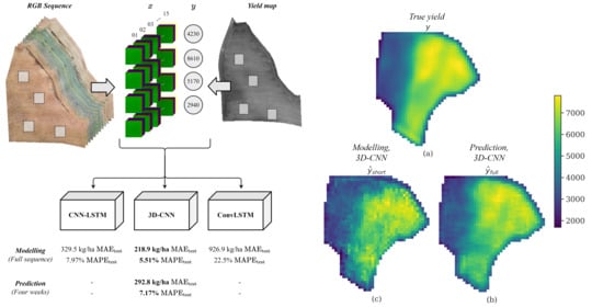
| CNN-LSTM | 456.1 | 329.5 | 7.97 | 0.905 | 2.94 × |
| ConvLSTM | 1190.3 | 926.9 | 22.47 | 0.349 | 9.03 × |
| 3D-CNN | 289.5 | 219.9 | 5.51 | 0.962 | 7.48 × |
| Model | Test RMSE (kg/ha) | ||||
|---|---|---|---|---|---|
| Min | 25% | 50% | 75% | Max | |
| CNN-LSTM | 456.1 | 655.1 | 1475.6 | 1623.7 | 2.152× |
| ConvLSTM | 1190.3 | 1477.8 | 1646.6 | 8750.2 | 1.334 × |
| 3D-CNN | 289.5 | 1355.4 | 1493.6 | 1649.0 | 1.926 × |
| Hyperparameter | Pre-CNN | CNN-LSTM | ConvLSTM | 3D-CNN |
|---|---|---|---|---|
| LSTM Architectural parameters | ||||
| LSTM layers | - | 2 | 2 | - |
| Dropout | - | 0.5027 | 0.9025 | - |
| Bidirectional | - | 0 | 1 | - |
| CNN Architectural parameters | ||||
| CNN layers | 6 * | - | 1 | 5 |
| Batch normalization | Yes * | - | No | No |
| Kernels | 128/64 * | - | 32 | 32 |
| Optimizer parameters | ||||
| Learning rate | 1.000 × | 7.224 × | 1.361 × | 1.094 × |
| L2-regularization | 0.9 * | 0.0 | 0.0 | 0.0 |
| Weeks in Input Sequence | Test RMSE (kg/ha) | Test MAE (kg/ha) | Test MAPE (%) | Test R - |
|---|---|---|---|---|
| 21, 22, 23, 24, 25 | 413.8 | 320.6 | 7.04 | 0.921 |
| 21, 22, 23, 24 | 393.9 | 292.8 | 7.17 | 0.929 |
| 22, 23, 24, 25 | 439.3 | 343.0 | 7.90 | 0.911 |
| 21, 22, 23 | 543.5 | 421.4 | 10.02 | 0.864 |
| 23, 24, 25 | 425.0 | 326.6 | 8.25 | 0.917 |
| 21, 23, 25 | 478.1 | 369.3 | 8.72 | 0.895 |
Publisher’s Note: MDPI stays neutral with regard to jurisdictional claims in published maps and institutional affiliations. |
© 2020 by the authors. Licensee MDPI, Basel, Switzerland. This article is an open access article distributed under the terms and conditions of the Creative Commons Attribution (CC BY) license (http://creativecommons.org/licenses/by/4.0/).
Share and Cite
Nevavuori, P.; Narra, N.; Linna, P.; Lipping, T. Crop Yield Prediction Using Multitemporal UAV Data and Spatio-Temporal Deep Learning Models. Remote Sens. 2020, 12, 4000. https://doi.org/10.3390/rs12234000
Nevavuori P, Narra N, Linna P, Lipping T. Crop Yield Prediction Using Multitemporal UAV Data and Spatio-Temporal Deep Learning Models. Remote Sensing. 2020; 12(23):4000. https://doi.org/10.3390/rs12234000
Chicago/Turabian StyleNevavuori, Petteri, Nathaniel Narra, Petri Linna, and Tarmo Lipping. 2020. "Crop Yield Prediction Using Multitemporal UAV Data and Spatio-Temporal Deep Learning Models" Remote Sensing 12, no. 23: 4000. https://doi.org/10.3390/rs12234000