Article

InSAR 3-D Coseismic Displacement Field of the 2015 Mw 7.8 Nepal Earthquake: Insights into Complex Fault Kinematics during the Event

1
State Key Laboratory of Earthquake Dynamics, Institute of Geology, China Earthquake Administration, Beijing 100029, China
2
Guangdong Provincial Key Laboratory of Geodynamics and Geohazards, School of Earth Sciences and Engineering, Sun Yat-Sen University, Guangzhou 510275, China
*
Author to whom correspondence should be addressed.
Remote Sens. 2020, 12(23), 3982; https://doi.org/10.3390/rs12233982
Submission received: 10 November 2020 / Revised: 19 November 2020 / Accepted: 1 December 2020 / Published: 5 December 2020
(This article belongs to the Section Remote Sensing in Geology, Geomorphology and Hydrology)

Abstract

:
The 2015 Mw 7.8 Gorkha, Nepal, earthquake occurred in the central Himalayan collisional orogenic belt, which demonstrated complex fault kinematics and significant surface deformation. The coseismic deformation has been well documented by previous studies using Global Positioning System (GPS) and Interferometric Synthetic Aperture Radar (InSAR) data. However, due to some limitations of spatially sparse GPS stations and InSAR only-one-dimensional observation in the line-of-sight (LOS) direction, the complete distribution and detailed spatial variation of the three-dimensional surface deformation field are still not fully understood. In this study, we reconstructed the three-dimensional coseismic deformation fields using multi-view InSAR observations and investigated the refined surface deformation characteristics during this event. We firstly obtained four ascending and descending InSAR coseismic deformation maps from both Sentinel-1A/B and ALOS-2 data. Secondly, we obtained the synthetic north-south deformation field from our best-fitting slip distribution inversions. Finally, we calculated three-dimensional deformation fields, which were consistent with coseismic GPS displacements but with higher resolution. We found that the surface deformation is dominated by horizontal southward motion and vertical uplift and subsidence, with minor east-west deformation. In the north-south direction, the whole deformation area reaches at least 150 × 150 km with a maximum displacement of ~1.5 m. In the vertical direction, two areas, including uplift in the south and subsidence in the north, are mapped with a peak displacement of 1.5 and −1.0 m, respectively. East-west deformation presented a four-quadrant distribution with a maximum displacement of ~0.6 m. Complex thrusting movement occurred on the seismogenic fault; overall, there was southward push motion and wave-shaped fold motion.

1. Introduction

On 25 April 2015, an Mw 7.8 earthquake occurred ~77 km northwest of Kathmandu, Nepal, located in the central Himalayan tectonic belt. This was the largest seismic event in Nepal since the Mw 8.1 earthquake in 1934. The event ruptured along the strike for ~150 km to the southeast of the epicentre; the area suffered from significant seismic damage, including Kathmandu, resulting in a large number of casualties and numerous building collapses. Following the Mw 7.8 mainshock, two strong aftershocks (Mw 6.7 and Mw 6.6) and a sequence of small magnitude aftershocks occurred. On 12 May, 17 days after the mainshock, the largest aftershock (Mw 7.3) occurred in the northeast of the rupture zone (Figure 1) [1,2].
The Indian and Eurasian plates are currently converging at a rate of 30–40 mm/a, approximately half of which is absorbed by the Himalayan orogenic belt [3,4,5,6]. This long-term collision and high convergent rate process have caused the Himalayan mountains to rise continuously, leading to the formation of several structural belts extending over thousands of kilometers. The convergence of the Himalayan orogenic belt has ultimately manifested as permanent deformations from large earthquakes on the Himalayan main thrust fault [3,5]. Over the past few centuries, the Himalayan arc has experienced several great thrust earthquakes, including the Lo Mustang earthquake (Mw ~8.2) in 1505, the Shillong earthquake (Mw ~8.1) in 1897, the Kangra earthquake (Mw ~7.8) in 1905, the Bihar-Nepal earthquake (Mw ~8.1) in 1934, and the Assam earthquake (Mw ~8.6) in 1950 [5,6,7]. The 2015 Nepal earthquake occurred in the earthquake vacant zone between the rupture zones of the Bihar-Nepal earthquake in 1934 and the Lo Mustang earthquake in 1505 (Figure 1) [5,8].
The significant and large-scale coseismic deformation produced by this earthquake has been widely investigated and documented in numerous previous studies using GPS and/or Interferometric Synthetic Aperture Radar (InSAR) data. The rapid response of the geodetic community and large SAR datasets provided by both Sentinel-1 and ALOS-2 satellites are useful to understand the fault geometry of the seismogenic fault and the relationship between the earthquake and mountain building [1,2,3,4]. However, due to inevitable limitations of spatially sparse GPS observations and InSAR only-one-dimensional measurements in the line-of-sight (LOS) direction, the detailed features and its spatial variations of the three-dimensional surface deformation fields are still not fully addressed. In this paper, we generate and compile four ascending and descending InSAR coseismic deformation maps using both Sentinel-1A/B and ALOS-2 data, which covers the whole seismic area during the 2015 Gorkha earthquake and facilitates our subsequent three-dimensional displacement decomposition. To acquire the prior information in the south-north direction due to the LOS north-south insensitivity, we aim to derive the synthetic deformation field in the north-south direction by inverting for slip distribution constrained by multi-source InSAR observations. To eliminate some of the ambiguity related to one-dimensional LOS measurements, we focus on calculating three-dimensional deformation fields to gain improved insights into complex fault kinematic during the Gorkha earthquake.

2. Data and Methods

2.1. InSAR Data and Interferogram Processing Methods

In this study, we use C-band (radar wavelength of 5.6 cm) Sentinel-1A TOPS (Terrain Observation with Progressive Scans) images on both ascending and descending tracks, and L-band (radar wavelength of 23.6 cm) ALOS-2 ScanSAR images on a descending track and ALOS-2 swath images from an ascending track (Figure 1). Table 1 lists some detailed parameters of each interferometric pair. The perpendicular baseline for all interferometric pairs was less than 300 m, and the time interval of obtained interferograms was less than 100 days, which ensures good coherence of interferograms in this mountainous region near Nepal.
Interferometric processing was performed using the GAMMA software package [9]. The two-pass InSAR approach [10] was utilized to form interferograms. The effects of topography were removed from interferograms using a filled 3 arc-sec (~90 m) resolution Shuttle Radar Topography Mission (SRTM) digital elevation model (DEM) obtained from the Consultative Group on International Agricultural Research Consortium for Spatial Information (CGIAR-CSI, http://srtm.csi.cgiar.org). To improve the signal-to-noise ratio (SNR), interferograms were downsampled to 10 looks in azimuth and 2 looks in range and were filtered using an adaptive filter function based on the local fringe spectrum [11]. This filtering strategy efficiently removed high-frequency noise and made the phase unwrapping considerably more stable. Interferogram phase unwrapping was carried out using the minimum cost flow algorithm [12]. The chosen reference point for phase unwrapping was away from the deformation center. It is worth noting that S1A descending data does not cover the entire deformed area with only a single track, so mosaic adjacent track interferograms are required. To achieve good matching of adjacent track phase values, we first spliced the interferograms of adjacent tracks before phase unwrapping, and then took the average phase value of two tracks in their overlapping region. The S1A ascending coseismic deformation field was derived from the results of [13]. The ALOS-2 ascending coseismic deformation field was derived from the results of [14].

2.2. Coseismic Slip Distribution Inversion Method

After the Nepal earthquake, USGS and the Global Centroid Moment Tensor (GCMT) quickly produced a focal mechanism solution. Many other studies have also obtained the seismogenic fault geometry and coseismic slip model based on seismic waves, GPS data, and InSAR data [6,13,14,15,16]. Based on the focal mechanism solutions and previous research, we assumed a low-angle single-plane fault model consisting of a single fault segment, 210 km long, and 140 km wide, subdivided into 294 sub-faults, measuring 10 km along the strike and dip, evenly distributed along the fault plane. The geometry of the fault was fixed, with strike and dip angles of 285° and 7°, respectively. Data used for the inversion were the S1A and ALOS-2 InSAR coseismic deformation fields from ascending and descending tracks. The Okada elastic half-space dislocation model was used in the inversion process, and the constrained least squares method was used to solve the relationship between slip amount and coseismic deformation on the fault plane:
| | G s d | | 2 + β 2 | | H τ 2 | | 2 = m i n
where G is the Green function for the elastic half-space describing the relationship between the unit slip on the subfault patches and the observations on the surface, s is the slip amplitude on the fault plane, d is the actual observation value, β is the smoothing factor, H is the Laplacian second-order smoothing operator, and τ is the stress drop on the fault plane.
To improve the computation efficiency during inversion, we performed quadtree sampling on the InSAR coseismic deformation data to reduce the number (~2000 points for each interferograms) of InSAR observations. Considering that the spatial resolution and phase noise level of the different InSAR data used in the inversion is roughly equivalent, all InSAR data weights were set to 1.0.

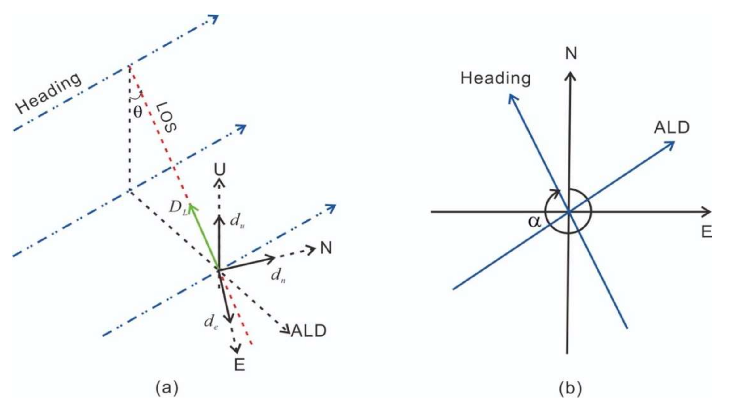
2.3. 3-D Displacement Decomposing Methodology

The conventional D-InSAR is capable of measuring only one-dimensional displacements along the radar LOS direction, which is the sum of the projection of three orthogonal components (vertical, north-south, and east-west) in three directions [17]. The relationship between the LOS displacement value and three displacement components is shown in Figure 2. According to the geometric relationship of the radar imaging, assuming LOS displacement is positive when ground motion of a target is close to the satellite, the relationship between the satellite LOS observations (D) and the vertical ( d u , up positive), north ( d n ), and east ( d e ) components can be expressed as:
D = d u cos θ i sin θ i d n cos ( α 3 π / 2 + d e sin ( α 3 π / 2 ) ]
where α is the orbit azimuth angle (positive clockwise from the north); α 3 π / 2 is the Azimuth Look Direction (ALD), equal to the angle between the range and north directions (positive clockwise); and θ i is the satellite incident angle of the ith pixel. The changes in incident angle between ALOS-2 descending and S1A ascending data are shown in Figure 3; the range of incident angles of radar data in the 3-D solution area was very large, with a fluctuation range of close to 10°. Therefore, our 3-D solution for the Nepal coseismic deformation field could not ignore the spatial variations of the incident angle for each pixel in SAR images.
For the same ground deformation field, the magnitude of an InSAR LOS observation is related to the flight direction and incident angle of the radar satellite. The smaller the angle of incidence, the more sensitive it is to the vertical deformation component; the larger the angle of incidence, the more sensitive it is to the horizontal deformation component. Single-orbit InSAR coseismic deformation fields have certain correlations with satellite parameters, causing problematic LOS blur in D-InSAR technology. Solving for the 3-D deformation field using multiple different sources and types of InSAR data is an effective way to solve this problem, with different studies proposing different solutions. Ref. [18] used four combinations of left and right views of ascending and descending InSAR data to obtain the 3-D deformation component of the 2002 Nenana Mountain M6.7 earthquake in Alaska. However, because it remains difficult to obtain SAR data for four different combinations in the same region, this method is not very practical. Ref. [19] combined D-InSAR technology on ascending and descending tracks and the azimuth pixel shift (AZO) technique to obtain the coseismic 3-D component of the 2003 Iranian Bam Mw 6.5 earthquake. Ref. [20] obtained the 3-D surface deformation of the 2005 Kashmir Mw 7.6 earthquake using the offset measurements method on ascending and descending tracks. Ref. [21] obtained the 3-D deformation field through the fusion of multiple-aperture interferometry (MAI) and D-InSAR technology; however, although this method can better constrain the azimuthal deformation, it suffers from low precision. Ref. [22] used ASAR ascending and descending data to combine the synthetic north–south component to obtain the 3-D coseismic deformation field of the 2003 Bam Mw 6.5 earthquake.
It can be seen from Equation (2) that if complete 3-D deformation information is to be obtained, LOS observation values from at least three different perspectives are required. For this earthquake, we constructed a 3-D deformation solution equation based on the data obtained from three different LOS directions: S1A ascending data, and ALOS-2 ascending and descending data:
D 3 × 1 = P 3 × 3 d 3 × 1
where D 3 × 1 is the matrix of LOS observations; P 3 × 3 is the coefficient matrix; and d 3 × 1 is the matrix of three unknown components. In theory, after obtaining three kinds of LOS observations, the three components of the surface deformation can be directly solved according to Equation (3). However, during the actual process, the method was not applicable, mainly because the angle between the flight directions of the S1A or ALOS-2 satellites and the north-south direction was between 10° and 13° (Table 1). The InSAR data are not sensitive to north-south deformation, while the Mw 7.8 Nepal event was a south-southwest thrust earthquake accompanied by large north-south coseismic displacement. We found that the error of the north-south component was very large, resulting in very large errors for the east-west and vertical components; thus, this method is not reliable in our case.
To solve the problem of large error in the north-south component of the direct solution, we simulated the 3-D component of the coseismic displacement field associated with the Nepal earthquake based on the Okada elastic dislocation model using the slip distribution inverted jointly by ALOS-2 and S1A data on ascending and descending tracks. The north-south component of the forward inversion was taken as the known value, and the 3-D components of the earthquake were calculated by combining the observational data for two different orbital types: ALOS-2 descending data and S1A ascending data.
The north-south component of the forward inversion was regarded as a known value, and the vertical and east-west components of any point can be expressed by Equation (4) according to Equation (2):
d u d e = cos θ 1 sin θ 1 sin α 1 cos θ 2 sin θ 2 sin α 2 1 D 1 D 2 + sin θ 1 cos α 1 sin θ 2 cos α 2 d N
where d u and d e are the vertical and east-west components to be solved; d N is the simulated north-south component from coseismic slip inversion; D 1 and D 2 are the LOS observations from ALOS-2 descending and the S1A ascending data, respectively; θ 1 and θ 2 are the incident angles of ALOS-2 descending and S1A ascending, respectively; and α 1 and α 2 are the angles between the heading directions of the ALOS-2 and S1A satellites and north, respectively.

3. Results

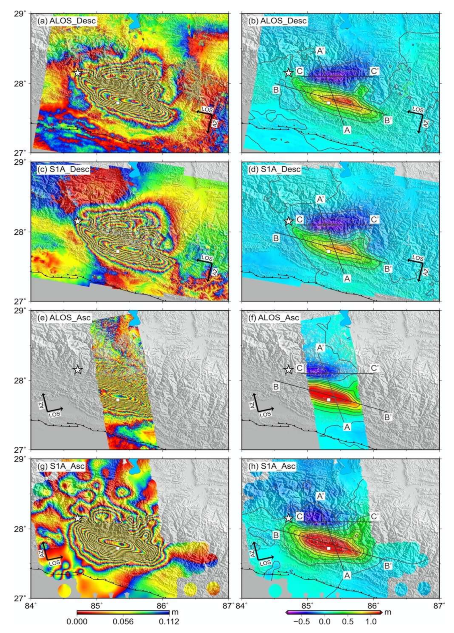
3.1. Coseismic Deformation Fields Acquired from Multi-Source InSAR Data

The coseismic deformation fields of the Nepal Mw 7.8 earthquake obtained from ALOS-2 and S1A data on ascending and descending tracks are shown in Figure 4. The four kinds of different InSAR data all obtained coseismic deformation fields with good coherence and complete spatial coverage. The four coseismic deformation fields show good similarities and consistency in the whole deformation pattern, each including two main deformation areas of uplift in the southern part and subsidence in the northern part. It indicated that vertical deformation was dominant, while east-west deformation was weak. Images from both ascending and descending tracks are viewed from the right side; therefore, if east-west deformation had been significant, the signs of the LOS deformation on the ascending and descending tracks would have been reversed. Among these, the descending interferometric fringe patterns (Figure 4a,c) and deformation fields (Figure 4b,d) of ALOS-2 and S1A data show the highest consistency; maximum uplift in the southern region is ~1.1 m, and maximum subsidence in the northern region is ~0.7 m. Moreover, uplift zones in the two descending deformation fields show obvious bulges on the east side, embedded in the subsidence zone in the north. The ascending interferometric fringe patterns (Figure 4e,g) and deformation fields (Figure 4f,h) of ALOS-2 and S1A data are also very similar; maximum uplift values in the southern region are ~1.5 m, and maximum subsidence values in the northern region are ~0.5 m; a convex uplift zone also appears on the eastern side. In addition, there is an obvious similarity between the descending and ascending deformation fields of S1A and ALOS-2 data (Figure 4), which indicates significant vertical movement characteristics of southern uplift and northern subsidence. However, the large scale and significant magnitude of the horizontal southward deformation field, and the displacement components in different directions, could not be obtained without a 3-D solution for the coseismic deformation field.
Although the two ascending deformation fields or the two descending deformation fields show overall consistency, they also show slight differences; furthermore, there are some differences between S1A and ALOS-2 descending data and their ascending data. In order to further reveal the fine distinction among the four deformation fields, we designed three profiles across the same location of the four deformation fields (Figure 5). It is clear that regardless of whether the tracks are ascending or descending, the morphology of the three profiles shows high consistency, but the displacement is slightly different. The deformation curves along the north-south profile (AA’) are similar in shape, but displacement values from the ascending datasets are larger than those of the descending datasets in the southern uplift area, whereas the opposite case applies in the northern subsidence area. On two near east-west profiles (BB’ and CC’), this offset variation among different datasets is more obvious. These differences may be due to different satellite incident angles, different post-earthquake times, and errors during processing. However, considering that the post-earthquake time of each interferometric pair was very close (within 6 days), it is likely that the differences are mainly due to variant sensitivities to vertical and horizontal deformation caused by different incident angles of the satellites. This also means that the coseismic deformation field obtained from single orbit InSAR is dependent on the data observation mode and the incident angle. Combining multi-platform, multi-LOS InSAR data to solve for the 3-D coseismic deformation field and surface displacement components, without relying on satellite data type, can improve our understanding of surface deformation and the movement of the seismogenic fault.

3.2. Comparative Analysis of Slip Distribution Inversion Results

In this study, we used different data combinations to invert the fault slip distribution and perform a comparative analysis of the inversion results. First, we used ALOS-2 and S1A single platform satellite ascending and descending data to invert the fault slip distribution, respectively (Figure 6a,b). Then we combined ALOS-2 and S1A ascending and descending data (i.e., four kinds of data) to perform joint inversion of multi-platform satellite data (Figure 6c). The slip distributions obtained using the different combinations show a high degree of consistency. The differences between the slip distribution inverted from the ALOS-2 and S1A data (Figure 6d) are generally within ±0.5 m, and are even smaller (within ±0.3 m) between the multi-platform inversion and the single platform inversion (Figure 6e,f). The inversion results from the multi-platform data are not significantly improved compared to the single platform. This shows that the single platform ascending and descending data can already provide a good constraint on fault slip distribution characteristics. In fact, although the multi-platform inversion provides more constraint information, there is a large degree of redundancy because the flight directions of different satellite platforms are relatively close and the incident angles of the radar are not very different; as such, the slip distribution results were not significantly improved.
Similar to the results of previous studies [6,13,14,15,16], the coseismic slip distribution was found to be a smooth continuous area with obvious uplift bulges at the north-eastern end. We compared the ALOS-2 descending coseismic deformation field with the slip distribution obtained from the joint inversion using ALOS-2 and S1A ascending (Figure 7). The result shows that the larger slip is distributed in the central region of the extreme seismic zone, and the maximum is located at the junction of the uplift zone and the subsidence zone. The inversion results show that the earthquake was a typical thrust-type event; rupture was concentrated between the epicentre and 150 km to the southeast and extended to a depth of 10–18 km. The average rake angle was 97° and the maximum slip amount was 5.6 m at a depth of 13 km. The calculated moment magnitude was Mw 7.8.
The simulated LOS coseismic deformation fields by the fault slip model constrained jointly by four kinds of data (both ALOS-2 and S1A descending and ascending) and their residuals, along with observed values, are shown in Figure 8. The deformation field simulation results obtained using a single platform joint inversion are basically consistent with that obtained by the multi-platform joint inversion. The simulated values of the InSAR coseismic deformation field obtained by the three different combinations are in good agreement with the actual observations; the fitting error is concentrated within ~10 cm, which indicates that the simulation results of the three combinations can well reflect the distribution characteristics of the actual observations.

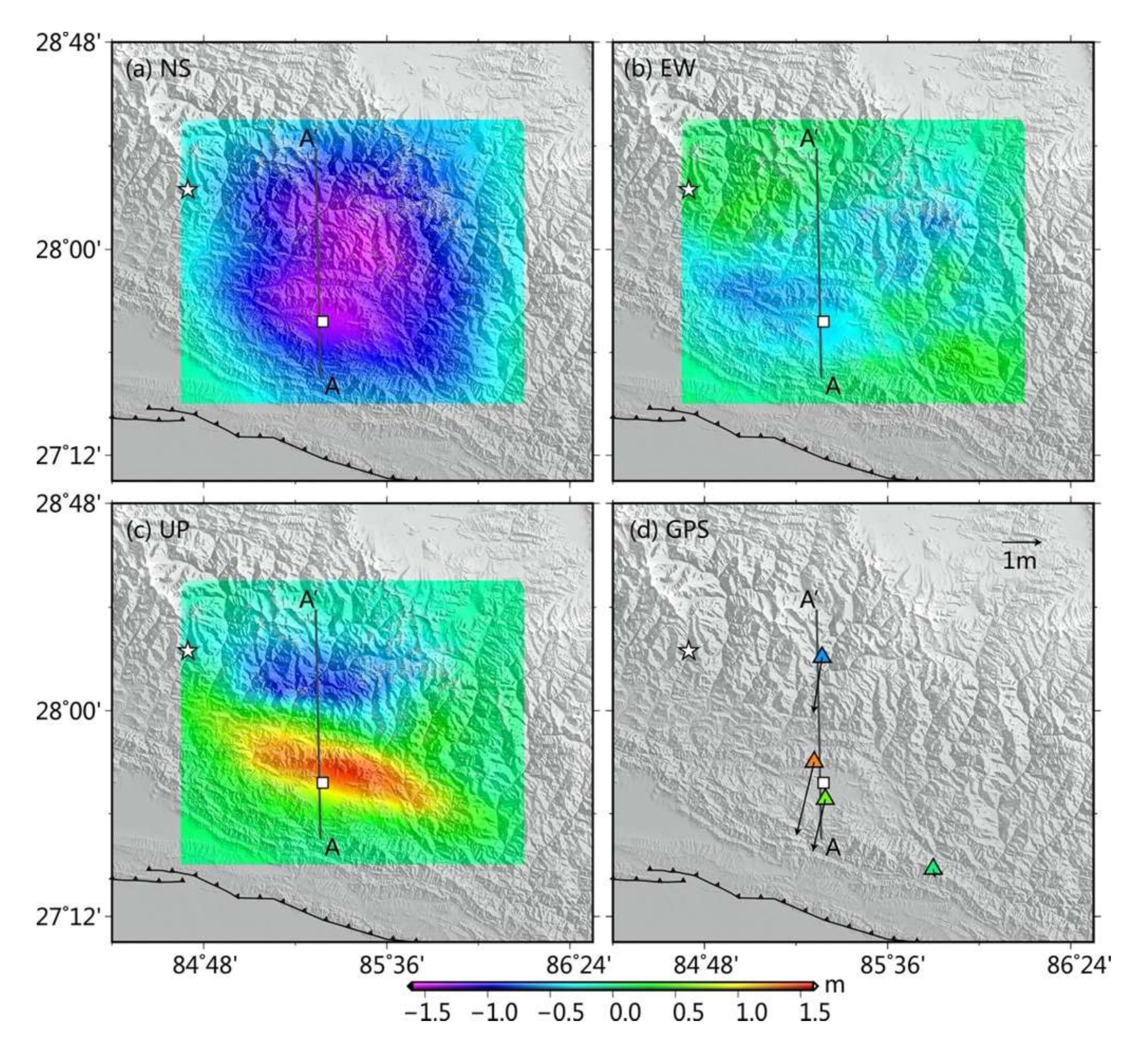
3.3. Analysis of 3-D Deformation Field

From Equation (4), we obtained the 3-D components of the Mw 7.8 Nepal earthquake deformation field (Figure 9). The results show that in the north-south direction it is characterized by southward deformation; in the central region, the displacement has a magnitude exceeding 1.5 m (Figure 9a). In the east-west direction, westward deformation of less than 0.5 m dominates, although there is smaller eastward displacement in the upper left and lower right corners of the solution area (Figure 9b). In the vertical direction, the shape of the deformation field is similar to that of the LOS deformation field, with two deformation centers: uplift of ~1.5 m in the south, and subsidence of ~1 m in the north (Figure 9c). Figure 9d shows horizontal and vertical displacements of three GPS points in our 3-D deformation solution area.
To analyze how much the 3-D deformation component of the Nepal earthquake contributed to the LOS displacement, we drew a near north-south profile (AA’ in Figure 9) and projected the 3-D deformation components and ALOS-2 descending LOS observation onto it (Figure 10). The shape of projection curve of the vertical component and the LOS deformation field show a high degree of consistency, and the magnitudes are also very close. However, for the east-west component with small deformation, and the north-south component with large deformation, the projection curves are very different from the LOS projection curves in both shape and magnitude. This indicates that LOS observations of the Nepal earthquake mainly reflect the vertical motion characteristics; the horizontal motion characteristics are not well reflected.
We combined the north-south component and the east-west component to obtain the horizontal deformation field of the earthquake (Figure 11). The horizontal deformation field has a dumbbell-shaped symmetrical distribution that can be roughly divided into left, central, and right regions. The deformation field on the left side is accompanied by a clockwise rotation; the central region is dominated by the southward movement roughly perpendicular to the MFT, and the right region is accompanied by a counter-clockwise rotation.
To understand the relationship between the horizontal motion and the seismogenic fault, we projected the horizontal deformation onto the directions perpendicular and parallel to the fault strike, respectively (Figure 12). The results show that in the region with large deformation, horizontal deformation was mainly in the perpendicular fault direction; there is no obvious deformation in the parallel fault direction. At the trailing edge of the extreme seismic zone, the parallel fault component appears to move from the two sides to the middle, whereas in the front, it moves from the middle to the sides. Overall, the horizontal deformation field has a dumbbell-shaped distribution. During the earthquake, the Kathmandu Basin shows a tendency to expand to the east and west sides.

4. Discussion

4.1. Comparison of 3-D Deformation Fields and GPS Data

To verify the accuracy of the 3-D deformation field results, we generated a near north-south profile (AA’ in Figure 9). We projected InSAR 3-D displacements and GPS observations [23] onto the profile and compared the difference between them (Figure 13, Figure 14a). It shows that our 3-D deformation field is in good agreement with the GPS 3-D displacement. The difference in each direction is mostly within ±5 cm, and only the north-south component at station KKN4, and the east-west component at station CHLM, have relatively large errors compared with the GPS observations (~0.3 m and 0.2 m, respectively). This indicates the feasibility and reliability of the method of resolving a 3-D deformation field combined with simulated values.
To verify whether the fault-slip model we obtained is reliable, we predicted the 3-D displacement component of the locations of all GPS stations in Figure 1a using our fault-slip model, and compared the predictions with the GPS observations. The results show that, generally, the GPS predictions and observations are in good agreement (Figure 14b), confirming that our model is reliable.

4.2. Significance of the 3-D Deformation Field and Characteristics of Fault Motion

The 3-D deformation field of the Nepal earthquake presented here confirms that the earthquake was mainly characterized by significant vertical deformation, with frontal uplift and rear settlement and overall southward movement. East-west deformation was weak. These results suggest that the complex movement of the seismogenic fault involves the whole southward motion and wavy-shaped fold of the upper plate. Ref. [24] proposed models for interseismic loading of Himalayan low-angle thrust faults, and coseismic ruptures of different magnitudes (Figure 15). The elastic strain of the upper crust accumulated during interseismic periods is finally released by irreversible fractures and permanent displacement on the main Himalayan fault (MHF). The MHF system may have several rupture modes, one of which is slightly smaller, with rupture and displacement mainly occurring at the bottom of the low and high Himalayan terrain steep slopes; however, ruptures do not reach the surface (Figure 15b). The 3-D deformation field derived in this study is in good agreement with the coseismic displacement image of the rupture mode, but there are also some differences. The overall southward translational motion associated with this earthquake cannot be well represented. Therefore, based on our results, we have improved the surface deformation model for this Nepal earthquake, as shown by the red dotted line in Figure 15b.

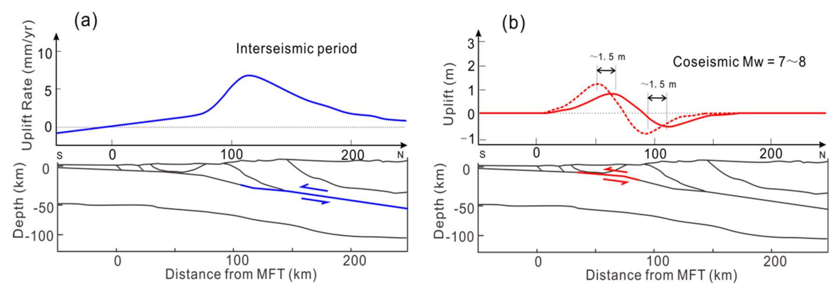
4.3. Large-Scale Low-Angle Thrust Earthquakes and Associated Lateral Extrusion and Tension

Our Nepal 3-D coseismic deformation results and analysis (Figure 11 and Figure 12) show that the southward horizontal displacement component perpendicular to the fault, dominates and was mainly distributed in the center area of the coseismic deformation field. In contrast, the near east-west horizontal displacement component parallel to faults is distributed on the periphery of the deformation field with smaller magnitude, but the values in the north part of the deformation center region converge to the center, and those in the south part deviate from the deformation center and expand in the east and west direction (Figure 12). This is also consistent with GPS observations (Figure 1). The GPS far-field observational displacements point to the deformation center area at the back edge of the coseismic deformation field, whereas at the front edge it deviates from the deformation center area. These phenomena indicate that the Nepal earthquake was accompanied by significant lateral compression inward at the rear end of the central deformation region and tension outward at the front edge. Here, we can further speculate that low-angle thrust-type earthquakes in the Himalayan seismic zone are accompanied by lateral intrusion and extrusion of material at the edges of the deformation fields.
In addition, our 3-D results also show the complementarity of coseismic displacement and interseismic deformation (Figure 16). The blue arrows in Figure 16 show the coseismic horizontal displacement field. The red arrows show the interseismic horizontal velocity field. The left image refers to the stable Eurasian plate. The right image refers to the Himalayan piedmont plain. Here we use the GPS stations in the blue triangle as a reference and obtain the interseismic velocity field relative to the piedmont plain. We can see that the interseismic velocity in the Himalayan orogenic belt is obviously smaller than that in the north, which indicates that the region is in a locked state during interseismic period, thus resulting in a displacement deficit and strain accumulation in the Himalaya orogenic belt. During an earthquake, the accumulated strain is released in whole or in part, which reflects the relationship of the deformations between interseismic and coseismic.

4.4. Applicability of Different 3-D Deformation Solutions to Earthquakes with a Large North–South Component

Because InSAR satellites have a near-polar orbit, the contribution of the north-south displacement to the LOS observation is much smaller than that of the vertical and east-west displacements. Therefore, in the 3-D solution, the accuracy of north-south deformation is often not sufficient to provide a reliable north-south displacement field. For the Nepal earthquake, we first attempted to solve the 3-D component directly using three different LOS observations, but the north-south direction error was very large, and the error of some pixels reached the meter level; as a consequence, the other two components also had large errors. Secondly, we attempted the offset tracking method. The obtained azimuth displacements were significantly different from the GPS results, and their accuracy was much lower than that of the LOS observations. Finally, we combined the LOS observations on ascending and descending tracks and the synthetic north-south deformation to obtain the 3-D deformation field of the earthquake, which was in good agreement with the GPS observations. The result suggests that for an earthquake with large north-south displacement, the method of combining LOS observations on ascending and descending tracks with synthetic north-south deformation can obtain a more reliable 3-D deformation field.

5. Conclusions

In this study, we obtained the coseismic deformation fields of the 2015 Nepal Mw 7.8 earthquake using four kinds of InSAR data on ALOS-2 and S1A ascending and descending tracks. The pattern of all of these deformation fields is similar, with an uplift in the south and subsidence in the north, although there are some slight differences among them. We studied the influence of different InSAR data combinations on the fault slip distribution inversion. The results show that joint inversion using multi-platform datasets did not significantly improve the model fitting compared to that constrained by data from the single platform for this earthquake. We resolved 3-D deformation fields for the 2015 Nepal earthquake by combining ALOS-2 descending data, S1A ascending data and the synthetic north-south deformation field. The results show this earthquake was dominated by vertical and southward deformation: the vertical deformation included trailing edge subsidence and leading-edge uplift; the north-south deformation had overall southward movement; and the east-west deformation was small.

Author Contributions

Conceptualization, C.Q. and X.S.; methodology, X.Q.; software, X.Q.; validation, D.Z. and W.G., L.Z. and C.Q.; formal analysis, X.Q.; data curation, X.Q.; writing—original draft preparation, X.Q. and D.Z.; writing—review and editing, X.Q., Y.L. and C.Q.; visualization, X.Q.; supervision, C.Q. and X.S.; project administration, C.Q. and X.S.; funding acquisition, C.Q. and X.S. All authors have read and agreed to the published version of the manuscript.

Funding

This work was supported by the Basic Scientific Funding of the Institute of Geology, China Earthquake Administration [grant number IGCEA1809], the National Natural Science Foundation of China [grant number 41872229], and the National Key Technologies R&D Program [grant number 2018YFC1503602].

Acknowledgments

We would like to thank the European Space Agency (ESA) for providing Sentinel-1A (S1A) data, the Japan Aerospace Exploration Agency (JAXA) for providing Advanced Land Observing Satellite (ALOS)-2 data, Wang Kang for providing ALOS-2 ascending deformation field data, and Raphaël Grandin for providing S1A ascending deformation field data. Some Figures were prepared using the public domain Generic Mapping Tools (GMT).

Conflicts of Interest

The authors declare no conflict of interest.

References

  1. Elliott, J.R.; Jolivet, R.; González, P.J.; Avouac, J.P.; Hollingsworth, J.; Searle, M.P.; Stevens, V.L. Himalayan megathrust geometry and relation to topography revealed by the Gorkha earthquake. Nat. Geosci. 2016, 9, 174–180. [Google Scholar] [CrossRef] [Green Version]
  2. Whipple, K.X.; Shirzaei, M.; Hodges, K.V.; Arrowsmith, J.R. Active shortening within the Himalayan orogenic wedge implied by the 2015 Gorkha earthquake. Nat. Geosci. 2016, 9, 711–716. [Google Scholar] [CrossRef]
  3. Ader, T.; Avouac, J.-P.; Liu-Zeng, J.; Lyon-Caen, H.; Bollinger, L.; Galetzka, J.; Genrich, J.; Thomas, M.; Chanard, K.; Sapkota, S.N.; et al. Convergence rate across the Nepal Himalaya and interseismic coupling on the Main Himalayan Thrust: Implications for seismic hazard. J. Geophys. Res. Solid Earth 2012, 117, B04403. [Google Scholar] [CrossRef] [Green Version]
  4. Bilham, R.; Larson, K.; Freymueller, J. GPS measurements of present-day convergence across the Nepal Himalaya. Nature 1997, 386, 61–64. [Google Scholar] [CrossRef]
  5. Liu, J.; Ji, C.; Zhang, J.Y.; Zhang, J.Y.; Zhang, P.Z.; Zeng, L.S.; Li, Z.F.; Wang, W. Tectonic setting and general features of coseismic rupture of the 25 April, 2015 Mw 7.8 Gorkha, Nepal earthquake. China Sci. Bull. 2015, 60, 2640–2655. (In Chinese) [Google Scholar] [CrossRef] [Green Version]
  6. Feng, G.; Li, Z.; Shan, X.; Zhang, L.; Zhang, G.; Zhu, J. Geodetic model of the 2015 April 25 Mw 7.8 Gorkha Nepal Earthquake and Mw 7.3 aftershock estimated from InSAR and GPS data. Geophys. J. Int. 2015, 203, 896–900. [Google Scholar] [CrossRef] [Green Version]
  7. Sapkota, S.N.; Bollinger, L.; Klinger, Y.; Tapponnier, P.; Gaudemer, Y.; Tiwari, D. Primary surface ruptures of the great Himalayan earthquakes in 1934 and 1255. Nat. Geosci. 2013, 6, 71–76. [Google Scholar] [CrossRef]
  8. Shan, X.J.; Zhang, G.H.; Wang, C.S.; Li, Y.C.; Qu, C.Y.; Song, X.G.; Yu, L.; Liu, Y.H. Joint inversion for the spatial fault slip distribution of the 2015 Nepal Mw 7.9 earthquake based on InSAR and GPS observations. Chinese J. Geophys. 2015, 58, 4266–4276. (In Chinese) [Google Scholar] [CrossRef]
  9. Werner, C.; Wegmüller, U.; Strozzi, T.; Wiesmann, A. GAMMA SAR and interferometric processing software. In Proceedings of the ERS-Envisat Symposium, Gothenburg, Sweden, 16–20 October 2000. [Google Scholar]
  10. Rosen, P.A.; Hensley, S.; Joughin, I.R.; Li, F.K.; Madsen, S.N.; Rodriguez, E.; Goldstein, R.M. Synthetic aperture radar interferometry. Proc. IEEE 2000, 88, 333–380. [Google Scholar] [CrossRef]
  11. Goldstein, R.M.; Werner, C.L. Radar Interferogram Filtering for Geophysical Applications. Geophys. Res. Lett. 1998, 25, 4035–4038. [Google Scholar] [CrossRef] [Green Version]
  12. Costantini, M. A novel phase unwrapping method based on network programming. IEEE Trans. Geosci. Remote Sens. 1998, 36, 813–821. [Google Scholar] [CrossRef]
  13. Grandin, R.; Vallée, M.; Satriano, C.; Lacassin, R.; Klinger, Y.; Simoes, M.; Bollinger, L. Rupture process of the Mw = 7.9 2015 Gorkha earthquake (Nepal): Insights into Himalayan megathrust segmentation. Geophys. Res. Lett. 2015, 42, 8373–8382. [Google Scholar] [CrossRef] [Green Version]
  14. Wang, K.; Fialko, Y. Slip model of the 2015 Mw 7.8 Gorkha (Nepal) earthquake from inversions of ALOS-2 and GPS data. Geophys. Res. Lett. 2015, 42, 7452–7458. [Google Scholar] [CrossRef]
  15. Lindsey, E.O.; Natsuaki, R.; Xu, X.; Shimada, M.; Hashimoto, M.; Melgar, D.; Sandwell, D.T. Line-of-sight displacement from ALOS-2 interferometry: Mw 7.8 Gorkha Earthquake and Mw 7.3 aftershock. Geophys. Res. Lett. 2015, 42, 6655–6661. [Google Scholar] [CrossRef]
  16. Li, Y.S.; Shen, W.H.; Wen, Y.M.; Zhang, J.; Li, Z.; Jiang, W.; Luo, Y. Source parameters for the 2015 Nepal Earthquake revealed by InSAR observations and strong ground motion simulation. Chin. J. Geophys. 2016, 59, 1359–1370. (In Chinese) [Google Scholar] [CrossRef]
  17. Wen, S.; Shan, X.; Zhang, Y.; Wang, J.; Zhang, G.; Qu, C.; Xu, X. Three-dimensional coseismic deformation acquisition and source characteristics analysis of Qaidam earthquake based on InSAR. Chin. J. Geophs. 2016, 59, 912–921. (In Chinese) [Google Scholar]
  18. Wright, T.J.; Parsons, B.E.; Lu, Z. Toward mapping surface deformation in three dimensions using InSAR. Geophys. Res. Lett. 2004, 31, L01607. [Google Scholar] [CrossRef] [Green Version]
  19. Fialko, Y.; Sandwell, D.; Simons, M.; Rosen, P. Three dimensional Deformation caused by the BAM, Iran, earthquake and the origin of shallow slip deficit. Nature 2005, 435, 295–299. [Google Scholar] [CrossRef]
  20. Wang, H.; Ge, L.; Xu, C.J.; Du, Z. 3-D coseismic displacement Field of the 2005 Kashmir earthquake inferred from satellite radar imagery. Earth Planet. Space 2007, 59, 343–349. [Google Scholar] [CrossRef] [Green Version]
  21. Bechor, N.B.D.; Zebker, H.A. Measuring two-dimensional movements using a single InSAR pair. Geophys. Res. Lett. 2006, 33, L16311. [Google Scholar] [CrossRef] [Green Version]
  22. Sun, J.B.; Liang, F.; Xu, X.W.; Gong, P. 3-D co-seismic deformation field of the Bam Earthquake (Mw 6.5) from ascending and descending pass ASAR radar interferometry. J. Remote Sens. 2006, 10, 489–496. (In Chinese) [Google Scholar]
  23. Su, X.N.; Wang, Z.; Meng, G.J.; Xu, W.Z.; Ren, J.W. Pre-seismic strain accumulation and co-seismic deformation of the 2015 Nepal Ms 8.1 earthquake observed by GPS. China Sci. Bull. 2015, 60, 2115–2123. (In Chinese) [Google Scholar] [CrossRef] [Green Version]
  24. Avouac, J.P. Mountain building: From earthquakes to geological deformation. Dynamic processes in extensional and compressional settings. Treatise Geophys. 2015, 6, 377–439. [Google Scholar]
  25. Zheng, G.; Wang, H.; Wright, T.J.; Lou, Y.; Zhang, R.; Zhang, W.; Shi, C.; Huang, J.; Wei, N. Crustal deformation in the India-Eurasia collision zone from 25 years of GPS measurements. J. Geophys. Res. Solid Earth 2017, 122, 9290–9312. [Google Scholar] [CrossRef]
Figure 1. Tectonic map of the 2015 Mw 7.8 Nepal earthquake. (a) Tectonic setting of the Mw 7.8 Nepal earthquake. Red stars denote epicentres of the Mw 7.8 main shock and the largest aftershock (Mw 7.3) reported by the United States Geological Survey (USGS). Green dots denote the distribution of aftershocks of Mw 4.0 or above before 29 June; yellow dots denote the aftershocks larger than Mw 6.0 (aftershock data from https://earthquake.usgs.gov/earthquakes/search/). Purple triangles denote Global Positioning System (GPS) stations; red and pink arrows show GPS horizontal displacement, and blue and light blue arrows show GPS vertical displacement. The black line with triangles denotes the Himalaya Frontal Thrust (MFT). The red dashed frame indicates the spatial coverage of Advanced Land Observing Satellite (ALOS)-2 data; the blue dashed frame indicates the spatial coverage of Sentinel-1A (S1A) data. The yellow line denotes the trace of the profile shown in (b). The yellow ellipses are the possible rupture range caused by the 1505 Lo Mustang earthquake and the 1934 Bihar-Nepal earthquake (modified after [3]). The white square indicates the location of Kathmandu. (b) Near north–south tectonic profile of the Himalaya seismic belt in the Nepal earthquake zone, as shown in (a) and modified after [5]. The light blue line denotes the rupture range of the Mw 7.8 earthquake.
Remotesensing 12 03982 g001
Figure 2. Geometric relationship between line-of-sight (LOS) displacement of the interferometric radar and three surface perpendicular deformation components. (a) Three-dimensional (3-D) imaging geometry of interferometric radar. (b) Horizontal projection of interferometric radar imaging.
Remotesensing 12 03982 g002
Figure 3. Incident angle distribution range of ALOS-2 descending (a) and S1A ascending data (b). Black box indicates 3-D solution areas; white stars denote the earthquake epicentre; white square shows the location of the city of Kathmandu; the black line segment with triangles denotes the Himalaya Frontal Thrust (MFT) fault.
Remotesensing 12 03982 g003
Figure 4. Coseismic interferograms and deformation fields of the Nepal Mw 7.8 earthquake acquired by Advanced Land Observing Satellite (ALOS)-2 and Sentinel-1A (S1A) data on ascending (Asc.) and descending (Desc.) tracks. (a,b) ALOS-2 descending interferogram and unwrapped deformation field. (c,d) S1A descending interferogram and unwrapped deformation field. (e,f) ALOS-2 ascending interferogram and unwrapped deformation field. (g,h) S1A ascending interferogram and unwrapped deformation field. Positive values are closer to the satellite direction. The contour interval is 0.2 m. White star denotes the epicentre position; white square denotes the location of Kathmandu; black line segments denote profile lines (AA’, BB’, CC’; see Figure 5) across the deformation field.
Remotesensing 12 03982 g004
Figure 5. Comparison of line-of-sight (LOS) deformation fields derived from S1A and ALOS-2 data on ascending and descending tracks along profiles AA’ (a), BB’ (b), CC’ (c) (see profile locations in Figure 4). ALOS-2 = Advanced Land Observing Satellite-2; S1A = Sentinel-1A.
Remotesensing 12 03982 g005
Figure 6. Comparison of slip distributions from inversions of different InSAR data combinations. (a) Slip distribution obtained from joint inversion of ALOS-2 ascending and descending data. (b) Slip distribution obtained from joint inversion of S1A ascending and descending data. (c) Slip distribution obtained from joint inversion of ALOS-2 and S1A ascending and descending data. (d) Differences in slip distribution between the inversion of ALOS-2 and S1A data. (e) Differences in slip distribution between the inversion of multi-platform satellite data and ALOS-2 data. (f) Differences in slip distribution between the inversion of multi-platform satellite data and S1A data.
Remotesensing 12 03982 g006
Figure 7. Comparison between the fault slip model of joint inversion using ALOS-2 and S1A ascending and descending data and the ALOS-2 descending coseismic deformation field. Gray curves show counters of slip moment. Blue dashed lines represent the depth of our fault model.
Remotesensing 12 03982 g007
Figure 8. Simulated deformation fields and fitting residuals between observations and models from joint inversions of ALOS-2 and S1A ascending and descending data. (a,d,g,j) are observations of four kind of data; (b,e,h,k) are their corresponding simulated values; and (c,f,i,l) are their corresponding residuals.
Remotesensing 12 03982 g008
Figure 9. Three-dimensional (3-D) deformation components of the Mw 7.8 Nepal earthquake. (a) North-south deformation component (positive to the north). (b) East-west deformation component (positive to the east). (c) Vertical deformation component (the upward direction is positive). (d) The triangle represents GPS stations with coded colors indicating the vertical deformation component and black arrow indicates the horizontal deformation component. The white star is the epicentre of the Nepal earthquake; the white square marks the location of Kathmandu. The line AA’ is the position of a profile.
Remotesensing 12 03982 g009
Figure 10. Comparison of three-dimensional (3-D) components and InSAR LOS observations of the Mw 7.8 Nepal earthquake. Blue, red, and green curves represent the 3-D components in the NS, EW, and UP directions, black curve shows the InSAR LOS displacement; the white square marks the location of Kathmandu. Profile location is seen in Figure 9.
Remotesensing 12 03982 g010
Figure 11. Three-dimensional (3-D) deformation field of the Mw 7.8 Nepal earthquake. The colored background shows the vertical deformation field; black arrows indicate the horizontal deformation field; white arrows represent GPS horizontal motion. Color-coded circles show the GPS vertical motion using the same color palette. The white star is the epicentre of the Nepal earthquake; the white square marks the location of Kathmandu.
Remotesensing 12 03982 g011
Figure 12. Fault-perpendicular and fault-parallel components of coseismic horizontal displacements. Blue arrows are the fault-perpendicular component; red arrows are the fault-parallel component; the purple line shows the surface projection of the up-dip edge of fault model; the white star denotes the epicenter; and the white square marks location of Kathmandu.
Remotesensing 12 03982 g012
Figure 13. Comparison between InSAR derived three-dimensional (3-D) displacements and the 3-D components of GPS observations. The green thick curves represent the InSAR 3-D solution results. Red dots indicate 3-D components of GPS. Profile location is seen in Figure 9.
Remotesensing 12 03982 g013
Figure 14. (a) Comparison of the solved three-dimensional (3-D) components with GPS observations. Different shapes represent different GPS stations. Different colors represent different components. Error bars represent the 95% confidence level. (b) Comparison between GPS predictions and observations. Different colors represent different components.
Remotesensing 12 03982 g014
Figure 15. Pattern of uplift during the interseismic period and the coseismic deformation field of the Mw 7.8 earthquake in Nepal (modified after [24]). (a) Pattern of uplift during the interseismic period, and associated stable-sliding portion of the fault at depth. (b) Pattern of uplift and subsidence at the surface associated with coseismic rupture of Mw 7~8 earthquakes (red solid curve). The red dotted line indicates the coseismic deformation of the Nepal earthquake obtained from the three-dimensional (3-D) solution.
Remotesensing 12 03982 g015
Figure 16. Comparison between the coseismic horizontal deformation field of the Nepal earthquake and the interseismic GPS horizontal velocity field. Red arrows denote interseismic GPS horizontal velocities [25]. Left image refers to the stable Eurasian plate. Right image refers to the Himalayan piedmont plain. Blue arrows denote coseismic horizontal displacement of the Nepal earthquake. White stars show the epicentre position; white squares are the location of Kathmandu.
Remotesensing 12 03982 g016
Table 1. InSAR data and parameters used in this study a.
SatelliteTrack and Orbit TypeImage ModeIncidence Angle (deg)Heading (deg)Reference Image Acquisition DateSecondary Image Acquisition DatePerpendicular Baseline (m)
S1AT19 DescendingTOPS31.3~46.5−167.4517 April 201529 April 201537.7
38.6
T21 Descending12 April 201506 May 2015154.0
24 April 201506 May 2015224.3
S1AT85 AscendingTOPS31.3~46.5−12.5209 April 201503 May 2015−203.3
ALOS-2T048 DescendingScanSAR26.8~49.7−169.9505 April 201503 May 20154.3
ALOS-2T157 AscendingSwath29.2~34.0−10.8721 Tuesday 201502 May 2015−118.6
a InSAR = Interferometric Synthetic Aperture Radar; S1A = Sentinel-1A; ALOS = Advanced Land Observing Satellite; TOPS = Terrain Observation with Progressive Scans.
Publisher’s Note: MDPI stays neutral with regard to jurisdictional claims in published maps and institutional affiliations.

