Modeling Gross Primary Production of Midwestern US Maize and Soybean Croplands with Satellite and Gridded Weather Data

Abstract

Gross primary production (GPP) is a useful metric for determining trends in the terrestrial carbon cycle. To estimate daily GPP, the cloud-adjusted light use efficiency model (LUEc) was developed by adapting a light use efficiency (LUE, ε) model to include in situ meteorological data and biophysical parameters. The LUEc uses four scalars to quantify the impacts of temperature, water stress, and phenology on ε. This study continues the original investigation in using the LUEc, originally limited to three AmeriFlux sites (US-Ne1, US-Ne2, and US-Ne3) by applying gridded meteorological data sets and remotely sensed green leaf area index (gLAI) to estimate daily GPP over a larger spatial extent. This was achieved by including data from four additional AmeriFlux locations in the U.S. Corn Belt for a total of seven locations. Results show an increase in error (RMSE = 3.5 g C m⁻² d⁻¹) over the original study in which in situ data were used (RMSE = 2.6 g C m⁻² d⁻¹). This is attributed to poor representation of gridded weather inputs (vapor pressure and incoming solar radiation) and application of gLAI algorithms to sites in Iowa, Minnesota, and Illinois, calibrated using data from Nebraska sites only, as well as uncertainty due to climatic variation. Despite these constraints, the study showed good correlation between measured and LUEc-modeled GPP (R² = 0.80 and RMSE of 3.5 g C m⁻² d⁻¹). The decrease in model accuracy is somewhat offset by the ability to function with gridded weather datasets and remotely sensed biophysical data. The level of acceptable error is dependent upon the scope and objectives of the research at hand; nevertheless, the approach holds promise in developing regional daily estimates of GPP.

1. Introduction

Gross primary production (GPP) in maize and soybean crops is an important measure for quantifying large scale carbon fluxes and plant productivity. GPP is defined as the total amount of carbon dioxide fixed by photosynthesis in a given area over a unit of time. GPP is a useful metric in determining the patterns and dynamics of the terrestrial carbon cycle [1] and it is essential in the study of ecosystem respiration and biomass accumulation [2]. The need to quantify the North American carbon sink necessitates precise carbon dioxide flux measurements [3] and while in situ data sources are available for this quantification, they represent field level data collection at specific locations. Extending GPP from field to regional scales can identify larger patterns and dynamics and helps quantify long-term carbon trends. Landscape level models created to derive an accurate estimation of GPP at regional scales for managed and unmanaged ecosystems at coarse temporal scales have varying degrees of accuracy; light use efficiency is at the core of these models. For example, Matsushita et al. [4] reported a 20% error in estimating annual NPP while Heinsch et al. [5] reported an 18% error. Heinsch et al. [6] found errors of 20–30% in estimates of annual GPP. Xiao et al. [7] reported errors in seasonally integrated GPP estimates of 3–20% while Cui et al. [1] reported root mean square errors (RMSE) of 2.97 g C m⁻² d⁻¹. Although Tramontana et al. [8] reported good agreement between estimated and observed GPP values when using only remotely sensed data, the best estimates of GPP were obtained when meteorological data were included with vegetation indices. Zhang et al. [9] provide a global GPP dataset for 2000-2016 (as an alternate to MOD17 GPP) based on a modified vegetation photosynthesis model (VPM GPP V20) driven by MODIS and climate data. The model utilizes ε, scalars for temperature and moisture, photosynthetically active radiation (PAR), and the energy absorbed chlorophyll. Yuan et al. [10] tested seven LUE-based models and found that models that incorporate environmental factors, including diffuse radiation, do not significantly underestimate GPP for cloudy days, unlike models excluding diffuse radiation. Zhang et al. [11] explained about 67% of tower-measured GPP accounting for the effect of diffuse radiation on ε.

Critically, many of the models referenced above do not estimate GPP at a daily temporal resolution. Running et al. [12] provide a daily estimate of GPP in the MOD17A2/A3 algorithm using global daily estimates of PAR (“a challenging problem”) and a biome lookup table to estimate light use efficiency. Based on LUE-based models for estimating GPP on a regional scale, the use of satellite imagery and modeled weather data, including diffuse radiation, is essential as monetary, personnel, time, and equipment constraints hinder collection of daily in situ data at a broad scale. The overall accuracy of models using satellite and modeled weather data input may be lower than those that utilize in situ field-level input. This is due in part to generalization of model parameters for application to heterogeneous regions, spatial and temporal restrictions of satellite data, and the accuracy of modeled weather input data. However, the ability to study large regions may offset loss of accuracy, depending upon research scope and objectives [1,4].

A daily light use efficiency model, known as the cloud-adjusted light use efficiency model (LUEc), introduced by Nguy-Robertson et al. [13], combines aspects of the Vegetation Photosynthesis Model (VPM) [7] and the LUE model [3]. The LUEc provides more reliable estimates of GPP by taking into account the effects of environmental and canopy factors (e.g., light quality, water availability, temperature, and phenology) on photosynthesis. This is achieved, using daily meteorological measurements and in situ green leaf area index (gLAI). Gitelson et al. [14] concluded that gLAI was preferable to total leaf area index, as nonphotosynthesizing portions of the canopy were not contributing to photosynthesis. Thus, in the LUEc, maximum light use efficiency (ε₀) is downregulated as environmental conditions change. Temperature, water stress, and phenology are used to estimate daily light use efficiency ε (e.g., [1,5,7,15]). However, to produce a more descriptive daily ε, the original study [13] based the scalars on in situ mass and energy flux measurements, micrometeorological observations and gLAI measurements to regulate ε₀.

The main objective of this study was to evaluate the potential applicability of the LUEc-enhanced four-scalar light use efficiency approach [13] to provide regional GPP estimates. This was accomplished using input data derived from remotely sensed satellite data and gridded weather datasets to estimate daily GPP over the entire growing season in seven U.S. Corn Belt agricultural sites. Thus, this study also investigates the robustness of the scalar stressor parameterizations identified in the original study [13] for regions outside eastern Nebraska. LUEc performance was evaluated by comparing estimated and AmeriFlux measured GPP values and calculating root mean squared error (RMSE) and mean normalized bias (MNB).

2. Materials and Methods

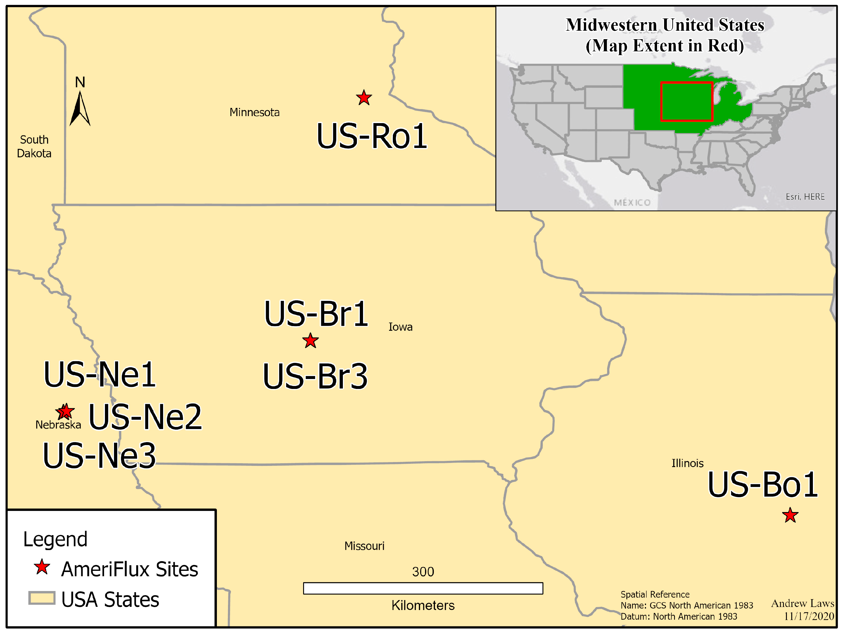
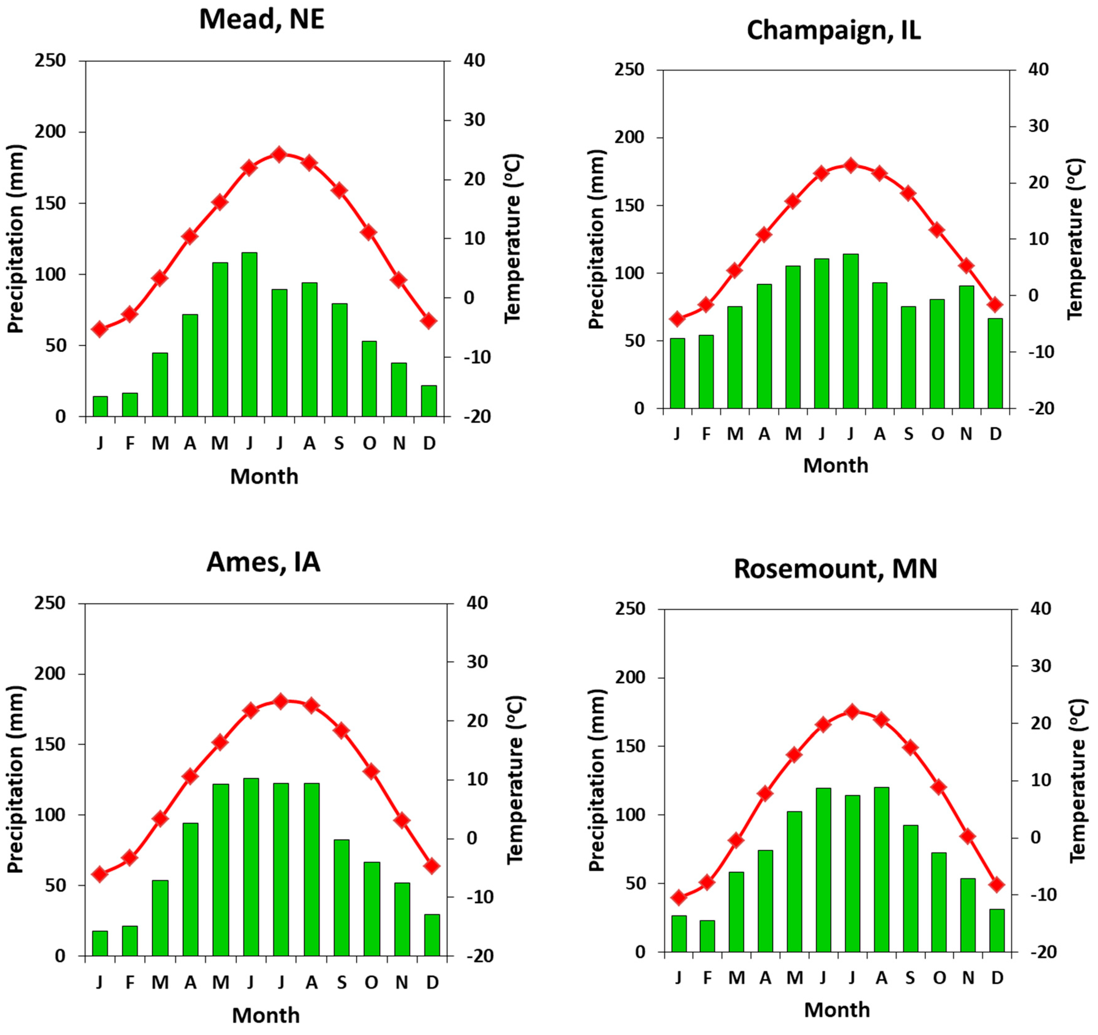
2.1. Study Site Summary

Data from seven AmeriFlux Midwestern agricultural sites in Nebraska, Illinois, Iowa, and Minnesota were used in this study (Figure 1 and

Table 1. AmeriFlux study site locations, management status, crop rotation, field years, mean annual temperatures, precipitation, and field area information. Coordinates and area determined from WGS 84 (EPSG:4326) system.

Approximate Field Site Location	AmeriFlux Site	Latitude, Longitude, Elevation	Management	Maize Crop	Soybean Crop	Mean Annual Temperature (°C)	Mean Annual Precipitation [+Irrigation] (mm)	Area (ha)
Mead, NE	US-Ne1	41.1650° N, 96.4766° W, 361 m	Irrigated	2002–2013	--	10	790 [+242]	49.8
	US-Ne2	41.1650° N, 96.4700° W, 362 m	Irrigated	2003–2013 Odd years; 2010, 2012	2002–2008 Even years	10	790 [+214]	53.5
	US-Ne3	41.1797° N, 96.4396° W, 363 m	Rainfed	2003–2013 Odd years	2002–2012 Even years	10	790	66.2
Brooks Field, near Ames, IA	US-Br1	41.9749° N, 93.6906° W, 313 m	Rainfed	2005–2011 Odd years	2006–2010 Even years	9	845	30.8
	US-Br3	41.9747° N, 93.6935° W, 313 m	Rainfed	2006–2010 Even years	2005–2011 Odd years	9	845	18.1
Bondville, IL	US-Bo1	40.0062° N, 88.2904° W, 219 m	Rainfed	2001–2007 Odd years	2002–2006 Even years	11	991	31.7
Rosemount, MN	US-Ro1	44.7143° N, 93.0898° W; 290 m	Rainfed	2005–2011 Odd years	2006–2012 Even years	6	879	17.7

). All sites are characterized by a humid continental climate (Dfa Koeppen climate classification) with hot humid summers and cold winters (Figure 2). The Nebraska sites are located at the University of Nebraska Eastern Nebraska Research and Extension Center near Mead, NE. All three Nebraska sites (US-Ne1, US-Ne2, and US-Ne3) have been under no-till or minimum-till management aside from initial disking conducted in 2001. Conservation-plow tillage has been in effect at US-Ne1 (only) since 2005. Only US-Ne1 and US-Ne2 are irrigated. Water applied was in accordance with best practices to reduce water stress and administer fertilizer, herbicide, and pesticides. The Illinois site, US-Bo1, is located approximately 12 km south of Champaign, Illinois. The site is not irrigated and is under no-till management administered by NOAA. The two Iowa Brooks Field sites, US-Br1 and US-Br3, are located approximately 8 km southwest of Ames, Iowa. The sites are not irrigated and are under a tillage management system typical throughout the Upper Midwest Corn Belt. The Minnesota Rosemount site, US-Ro1, is located approximately 24 km south of Saint Paul, Minnesota. This field is not irrigated and is under chisel plow tillage in the fall following maize harvest and in the spring after soybean harvest in the fall. US-Ro1 is managed jointly by the University of Minnesota and USDA.

Each site was equipped with an eddy covariance tower measuring key fluxes on a continuous basis. For these sensors, measurement heights were adjusted at each site (except US-Bo1) either once per season (US-Ne1, US-Ne2, US-Ne3) or at more frequent intervals (US-Ro1, US-Br1, US-Br3) based on crop height to keep the fetch area within the field during unstable, neutral, or moderately stable atmospheric conditions.

2.2. Input Data

2.2.1. Daymet Data

Daymet weather data were obtained from the Oak Ridge National Laboratory (ORNL) Distributed Active Archive Center (DAAC) Daymet (Version 2) [16]. The dataset was selected due to its relatively fine spatial resolution of 1 × 1 km. The dataset provides a grid of mosaicked gridded estimates of daily weather parameters. Parameters are generated using a network of ground observation sites to provide input data which is then interpolated and extrapolated using Daymet model algorithms. Daily data for respective years of the selected AmeriFlux study sites (referred to as “field years”) were extracted from the various sites using the “Single Pixel Extraction” tool (https://daymet.ornl.gov/dataaccess.html#SinglePixel) with specified latitude, longitude, and date range. Minimum temperature (Tmin, °C), maximum temperature (Tmax, °C), incoming shortwave radiation (Rg, J m⁻² d⁻¹), average vapor pressure (P, kPa), snow-water equivalent (kg m⁻²), precipitation (mm), and day length (s) were downloaded in CSV format in which average daily temperature, vapor pressure deficit, and incoming PAR were calculated in Microsoft Excel. Average daily temperature (T_avg) was calculated as:

Tavg = (Tmin + Tmax)/2

(1)

Vapor pressure deficit (VPD) was calculated using vapor pressure, P, as:

VPD = (0.61078 · exp[(17.269)(Tavg)])/(Tavg + 237.8) − P

(2)

Incoming PARin (µmol m⁻² d⁻¹) was calculated from incoming shortwave radiation (Rg) as:

PARin = Rg · 2.07

(3)

The constant 2.07 is computed as the product of the fraction of total shortwave at the top of the atmosphere, 0.45 Rg, J m⁻²d⁻¹ [17] and approximate energy conversion over the PAR range, 4.6 µmol J⁻¹ [18].

2.2.2. MODIS Data

MODIS v.5 eight-day composite surface reflectance (ρ) (products MOD09Q1 and MYD09Q1, Terra and Aqua, respectively) for band 1 (620–670 nm, ρ_red) and band 2 (841–876 nm, ρ_NIR) at 250 m spatial resolution were obtained using Google Earth Engine. Reflectances were used to calculate a wide dynamic range vegetation index (WDRVI) time series at eight day intervals as:

WDRVI = [α(ρNIR) − ρred]/[α(ρNIR) + ρred]

(4)

where α is a weighting parameter (typically 0.1–0.2 and set at 0.1 here). WDRVI is the normalized difference vegetation index (NDVI) when α equals 1; WRDVI equals zero when α equals (ρ_red/ρ_NIR) [19]. WDRVI values from the pixel nearest the geographic center of each field were used for analysis to avoid mixed pixels from adjacent areas due to the 250 m pixel resolution.

Green leaf area index (gLAI) values were estimated from the WDRVI time series following the approach of Nguy-Robertson et al. [20], with coefficients determined from ground samples at the Nebraska sites:

gLAI = 5.06 · (WDRVI value) + (−0.47) {Maize}

(5)

gLAI = 3.68 · (WDRVI value) + (−0.24) {Soybean}

(6)

The gLAI data were interpolated to continuous daily values for the growing season using Curve Expert 1.4 software (Hyams Development, https://www.curveexpert.net) and a cubic spline interpolation algorithm.

2.2.3. AmeriFlux Data

AmeriFlux (https://ameriflux.lbl.gov/) half-hourly or hourly GPP mean values were used to calibrate and validate the LUEc. GPP mean values were calculated from AmeriFlux half-hourly or hourly averages of net ecosystem exchange (NEE, µmol m⁻² s⁻¹) and ecosystem respiration (Re, µmol m⁻² s⁻¹). At all non-Nebraska sites NEE was assumed equal to canopy carbon dioxide flux (Fc, µmol m⁻² s⁻¹) as storage term calculations were not provided in these datasets and are likely small for these crop systems. NEE values were screened employing light response relationships. Values were graphed in relation to concurrent AmeriFlux measured half-hourly or hourly averages of PAR (µmol m⁻² s⁻¹) and a nonrectangular hyperbola model fitted to a period of five days. Outliers, typically more than three standard deviations from the model, were removed. For field years in which PAR was not provided, Equation (3) was used to approximate incident PAR fluxes using values of incoming solar radiation (Rg). Interpolation of daytime NEE and nighttime AmeriFlux measured ecosystem respiration (Re, µmol m⁻² s⁻¹) were then conducted. Half-hour averages were converted to half hour fluxes by multiplying the averages by 1800 s (half-hour)⁻¹; hourly averages were converted to hourly fluxes by multiply the averages by 3600 s h⁻¹. Daily GPP was determined as the sum of daily NEE (half-hourly NEE fluxes (hourly for Mead sites)) and daily Re (half-hourly Re fluxes (hourly for Mead sites)):

daily GPP = daily NEE − daily Re

(7)

where NEE and Re are positive when the flux is toward the surface. Daily GPP values are in units of g C m⁻² d⁻¹.

Field year growing season start dates were determined to be days in which daily GPP values commenced to be greater than zero and field year growing season end dates were determined to be days in which daily GPP values fell below the zero threshold.

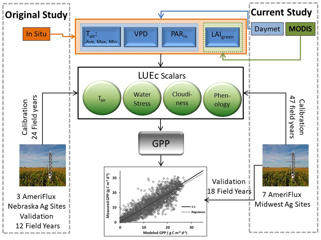
2.3. GPP Modeling Approach

The cloud-adjusted light use efficiency model (LUEc) [13] is an adaptation of the simple light use efficiency model of Monteith [21] based on earlier progressive work [3,7] to incorporate scalars to estimate daily GPP as:

daily GPP = ε₀ × C_scalar × T_scalar × W_scalar × P_scalar × APAR

(8)

ε₀ is the daily light use efficiency during clear sky conditions, APAR is the daily photosynthetically active photon flux absorbed by the green portion of the canopy (Equation (10)); the scalars account for the impact of diffuse light (C_scalar), air temperature (T_scalar), water stress (W_scalar), and phenology (P_scalar). ε₀ and the four scalars combined represent the well-known daily light use efficiency term, ε [21]:

daily GPP = ε × APAR

(9)

where

APAR = PAR_in × [1 − exp(−k × gLAI)]

(10)

Canopy extinction coefficients are the same as those used in the previous study [13] and are the average value of k for each crop when gLAI is greater than 1.5 m² m⁻² and dead LAI is less than 0.5 m² m⁻². Calculations of the scalars follow those previously mentioned using gridded Daymet and MODIS-derived LAI values instead of AmeriFlux on-site meteorological and biophysical observations as model input. This was done to meet our objective of evaluating the LUEc applicability in using input data derived from remotely sensed satellite data and gridded weather datasets to evaluate the potential to provide regional GPP estimates. A summary of each scalar is provided here but the reader is directed to Nguy-Robertson et al. [13] for details.

C_scalar. C_scalar accounts for the effects of diffuse lighting on photosynthesis [3]. Plants tend to use diffuse light more efficiently than direct sunlight. ε will increase on overcast days, where lighting is more diffuse than on clear days. C_scalar is calculated as:

C_scalar = a + β × [(PAR_d/PAR_in) − 0.17]

(11)

The term β is the sensitivity of daily light use efficiency to diffuse light and PAR_d is the diffuse PAR flux. As PAR_d is not commonly measured, the ratio PAR_d/PAR_in can be approximated using a cloudiness coefficient (CC) term [13]:

PAR_d/PAR_in = 1.08CC + 0.21

(12)

which is determined from PAR_in and PAR potential (PAR_pot):

CC = 1 − (PAR_in/PAR_pot)

(13)

PAR_pot refers to the estimated potential amount of incoming PAR flux, accounting for influences such as time of year, latitude, atmospheric pressure, and elevation as calculated by Weiss and Norman [17] with corrections reported in Nguy-Robertson et al. [13].

T_scalar. Initially developed by Raich et al. [22] in regions excluding croplands, T_scalar takes into account temperature effects on photosynthesis. The scalar is calculated using mean daily temperature, T_avg, calculated as the average of Daymet minimum and maximum temperatures. The constants for minimum temperature, maximum temperature, and optimal temperature (10, 48, and 28 °C, respectively) of Kalfas et al. [23] designed specifically with maize were used to define T_scalar as:

T_scalar = [(T_avg − 10) × (T_avg − 48)]/{[(T_avg − 10) × (T_avg − 48)] − (T_avg − 28)²}

(14)

while croplands were not examined in Raich et al. [22], values for ecoregions were consistent. Therefore, for this study, soybean optimal temperatures were assumed to be similar to those of maize.

W_scalar. The W_scalar accounts for water stress effects on photosynthesis and was calculated based on VPD using Equation (2) and associated constants [13]. This scalar was modeled by combining the approach of Wu et al. [24] and Maselli et al. [25], as water stress can be introduced through both atmospheric water deficits and soil water deficits. Unlike models in which the scalar remains constant until a critical threshold for VPD is reached, the LUEc approach has no threshold for VPD and the scalar was allowed to vary based on Daymet data.

σ_Wscalar is a term for the curvature parameter for water stress, proposed by Gilmanov et al. (2013) [26] to account for varying convexity in the relationship between photosynthesis and water stress:

W_scalar = exp{−[(VPD/σ_Wscalar)²]}.

(15)

While famers can irrigate to mitigate the impacts of VPD, the site-specific volume of applied water to a field is not inherent to the LUEc.

P_scalar. P_scalar accounts for leaf phenology, as immature leaves do not photosynthesize as efficiently as mature leaves, and leaves that are senescing do not have an optimal photosynthetic capacity [27,28]. The scalar is calculated using gLAI, a constant maximum gLAI value (gLAI_max) specific to each crop, and σ_Pscalar, the curvature parameter for the relationship between photosynthesis and phenology:

P_scalar = exp (−[((gLAI_max − gLAI)/(σ_Pscalar))²])

(16)

2.4. Calibration and Validation

Four basic steps were followed in this study:

(1)

Field Year Selection. For statistical purposes, 75% of field years were chosen randomly without replacement (i.e., 47 out of the 65 total field years) to calibrate the model (

Table 2. AmeriFlux calibration field years.

Calibration Years
Site	Maize	Soybean
US-Ne1 (NE—irrigated)	2002–2005, 2007, 2009–2012	--
US-Ne2 (NE—irrigated)	2003, 2005, 2007, 2009, 2010, 2013	2002, 2004, 2008
US-Ne3 (NE)	2003, 2005, 2011, 2013	2006, 2008, 2010, 2012
US-Br1 (IA)	2005, 2007, 2009	2006,2008
US-Br3 (IA)	2006, 2010	2007, 2009, 2011
US-Bo1 (IL)	2001, 2005, 2007	2002, 2004
US-Ro1 (MN)	2005, 2009, 2011	2006, 2010, 2012
Field Years	30	17

), to ensure at least one field year was reserved for each crop type for validation purposes for a total of 18 field years (

Table 3. AmeriFlux validation field years.

Validation Years
Site	Maize	Soybean
US-Ne1 (NE—irrigated)	2006, 2008, 2013	N/A
US-Ne2 (NE—irrigated)	2011, 2012	2006
US-Ne3 (NE)	2007, 2009	2002, 2004
US-Br1 (IA)	2011	2010
US-Br3 (IA)	2008	2005
US-Bo1 (IL)	2003	2006
US-Ro1 (MN)	2007	2008
Field Years	11	7

).

(2)

LUEc Calibration. The iterative training process using an R script as described in Nguy-Robertson et al. [13] was used to determine ε₀, β, σ_Wscalar, and σ_Pscalar values for irrigated and nonirrigated maize and soybean crops. The training utilized input values from the selected calibration field year flux data, Daymet derived T_avg, VPD, APAR, and T_scalar, and remotely-derived gLAI. The iterative process trained the parameters using a step-by-step method in which each scalar was estimated one at a time. During the iteration in which a parameter is calculated, assumptions are made about the other parameters to mimic optimal field conditions. Once the parameters are calculated, the iterations are repeated using the entire calibration dataset to produce ε_0, β, σ_Wscalar, and σ_Pscalar values with corresponding standard deviations. The calibrated dataset includes AmeriFlux-derived GPP, Daymet-derived T_avg, VPD, CC, APAR, and T_scalar, and remotely derived gLAI data. Additionally, gLAI_max values for irrigated and rainfed soybean and maize were estimated from MODIS-derived gLAI data (Equations (5) and (6)). From these outputs, scalars were calculated (Equations (8)–(15)).

(3)

Daily GPP Estimation. Data from validation field year datasets (Table 3) and parameters derived from the iterative process along with specified constants (

Table 4. Parameters for the calculation of scalars for the cloud-adjusted light use efficiency model (LUEc). The parameters in the upper portion of the table were calculated through the iterative process while those in the lower portion of the table are model constants from Nguy-Robertson et al. [13].

				Nguy-Robertson et al. [13]		This Study
Variables	Symbol	Equation	Units	Maize	Soybean	Maize	Soybean
Derived through iterative process:
Maximal light use efficiency	ε0	(8)	g C mol−1	0.526 ± 0.007	0.374 ± 0.005	0.573 ± 0.002	0.407 ± 0.002
Sensitivity of ε to diffuse light	β	(11)	unitless	0.347 ± 0.051	0.411 ± 0.056	0.181 ± 0.014	0.294 ± 0.020
Water stress curvature parameter	σWscalar	(14)	kPa	6 ± 0.25	4 ± 0	6 ± 0	4 ± 0
Phenology curvature parameter	σPscalar	(15)	m2 m−2	18 ± 4.59	18 ± 7.15	7 ± 0	8 ± 0
Calculated
Maximal green leaf area index [irrigated]	gLAImax	(10), (15)	m2 m−2	4.93 [6.78]	4.63 [6.15]	5.04 [5.14]	3.86 [4.25]
Constants
Light extinction coefficient	k	(10)	unitless	0.443	0.601	0.443	0.601
Minimum temperature for physiological activity	Tmin constant	(1), (13)	°C	10	10	10	10
Maximum temperature for physiological activity	Tmax constant	(1), (13)	°C	48	48	48	48
Optimal temperature for physiological activity	Topt constant	(13)	°C	28	28	28	28

), were used to calculate daily values of the scalars, C_scalar, W_scalar, and P_scalar (Equations (11), (14), and (15)) and APAR (Equation (10)), from which daily GPP values were estimated (Equation (8)).

(4)

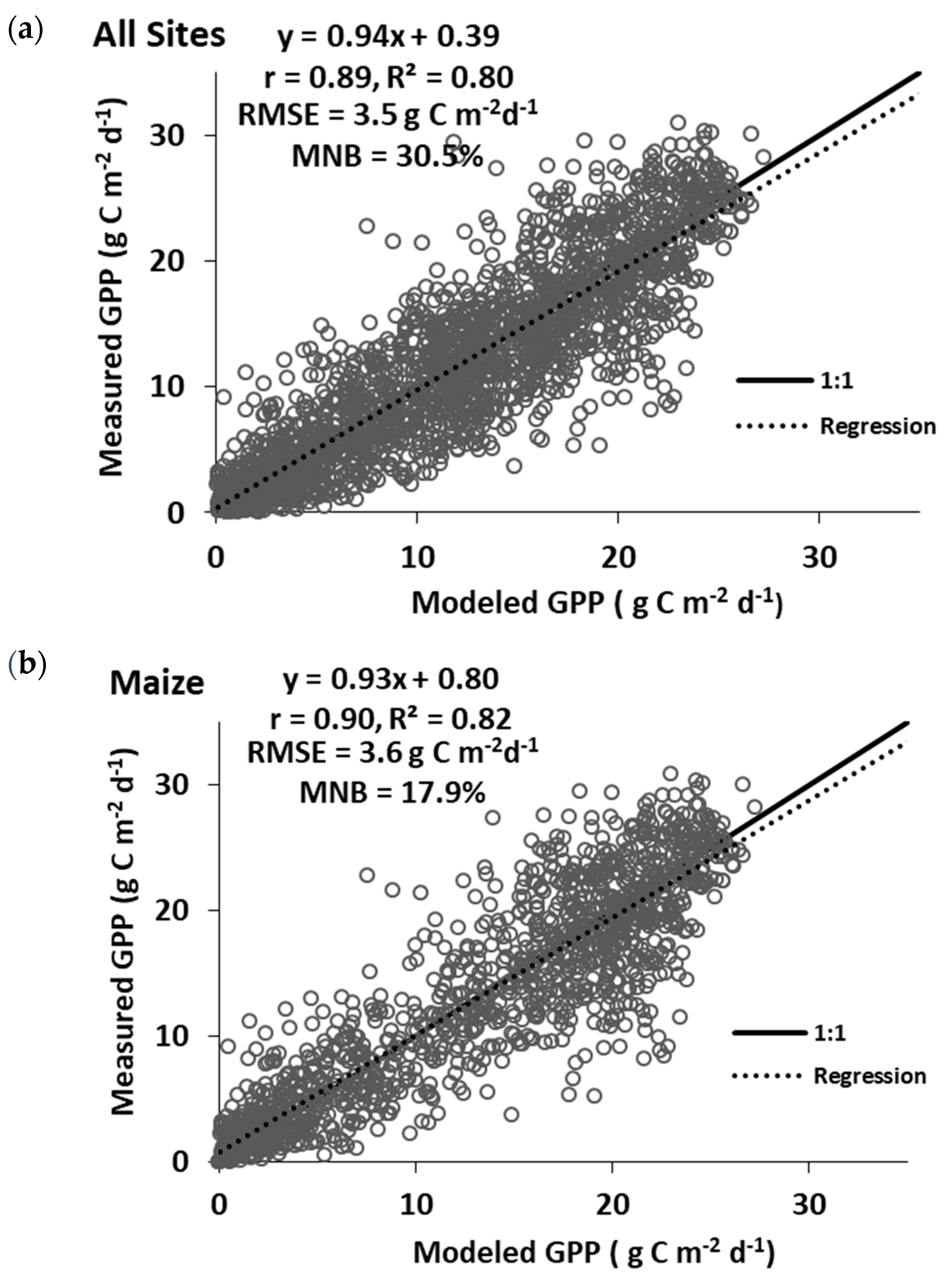
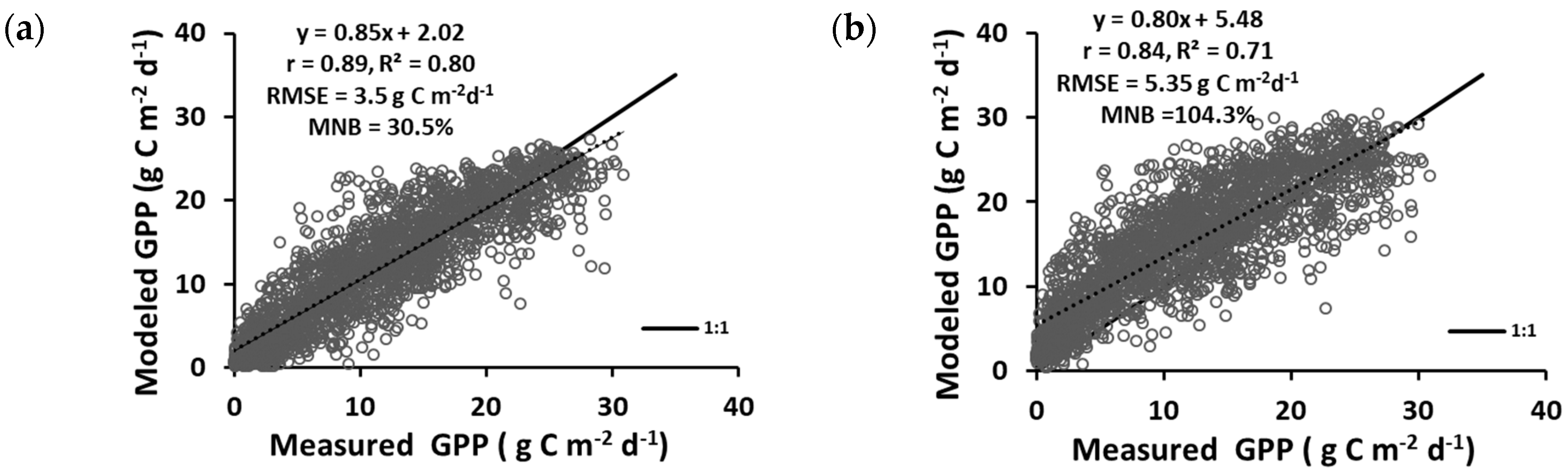
LUEc Validation. The estimated daily GPP values were compared to the observed AmeriFlux determined daily GPP using linear regression (α = 0.05), with corresponding R², root mean square error (RMSE), and mean normalized bias (MNB).

3. Results

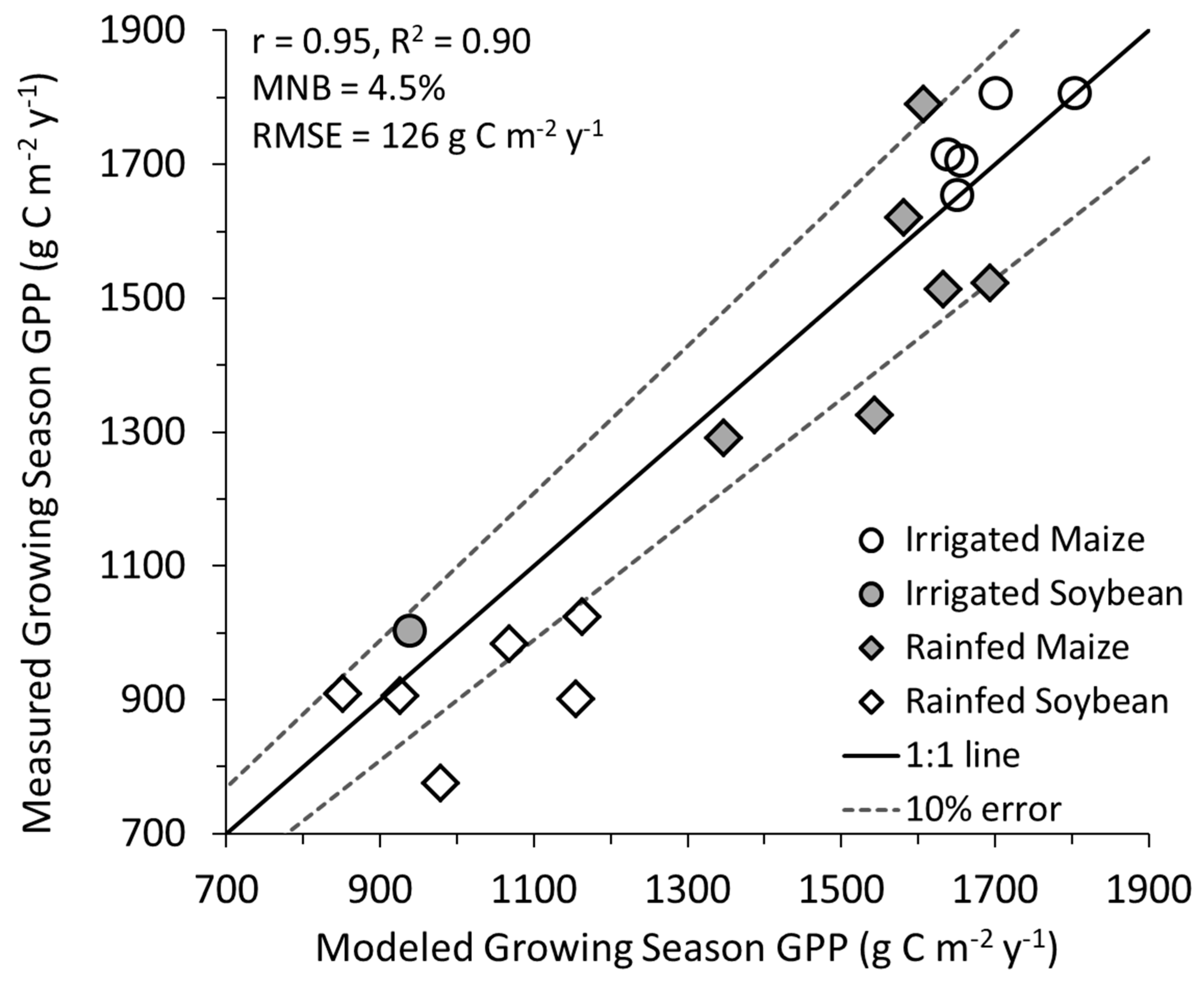
3.1. All Sites Years Combined

The parameters ε_0, β, σ_Wscalar, σ_Pscalar, and gLAI_max used to drive the LUEc, differed slightly from those reported previously [13] (Table 4). By using field years from geographically separated locations in the calibration process, the parameters were generalized to best fit conditions across all study locations of the northern Midwest region rather than just for the Nebraska sites as in the original Nguy-Robertson et al. [13] study.

Daily GPP for maize and soybean for the selected validation field years (Table 3), estimated using calculated daily values of C_scalar, W_scalar, and P_scalar, and APAR, were compared to observed AmeriFlux-determined daily GPP and indicate a strong correlation (r = 0.89; R² = 0.80), a slope of 0.93 ± 0.02, and an overall RMSE of 3.5 g C m⁻² d⁻¹ (Figure 3a) for all field years; however, the MNB was 30.5%. The results varied with crop. RMSE for overall maize field years was 3.7 g C m⁻² d⁻¹ (r = 0.90; R² = 0.82, and slope of 0.93 ± 0.02), with a MNB of 17.9% (Figure 3b) while RMSE for overall soybean field years was 3.2 g C m⁻² d⁻¹ (r = 0.80; R² =0.64, and a slope of 0.89 ± 0.05) with a MNB of 53.6% (Figure 3c). Residual plots did not highlight any potential issues with the data and demonstrated data were of a normal distribution.

In a measure of cumulative bias, growing season GPP-modeled values agreed with measured growing season values (RMSE = 126 g C m⁻² y⁻¹; r = 0.95; R² = 0.90; and MNB of 4.5%) (Figure 4).

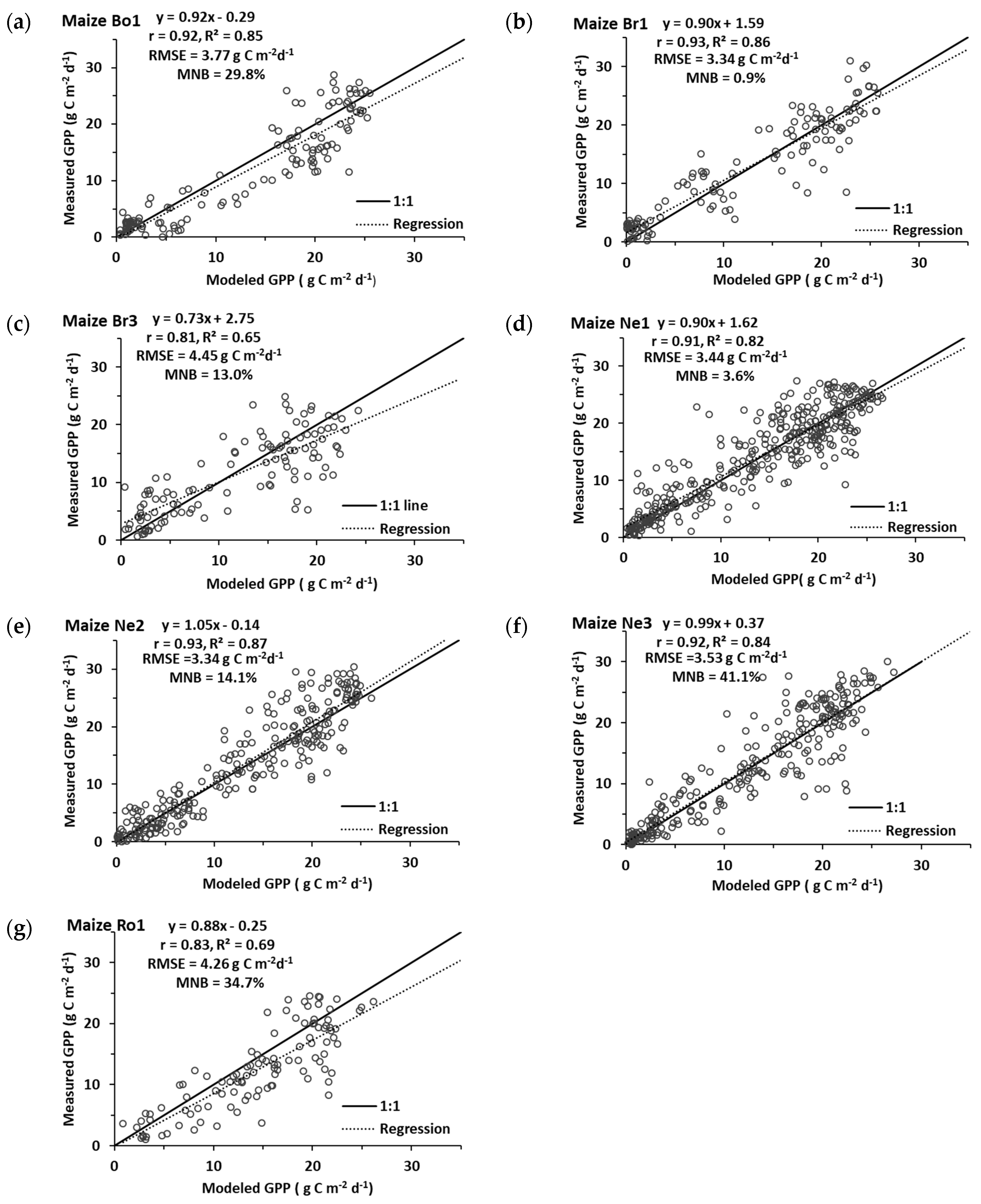
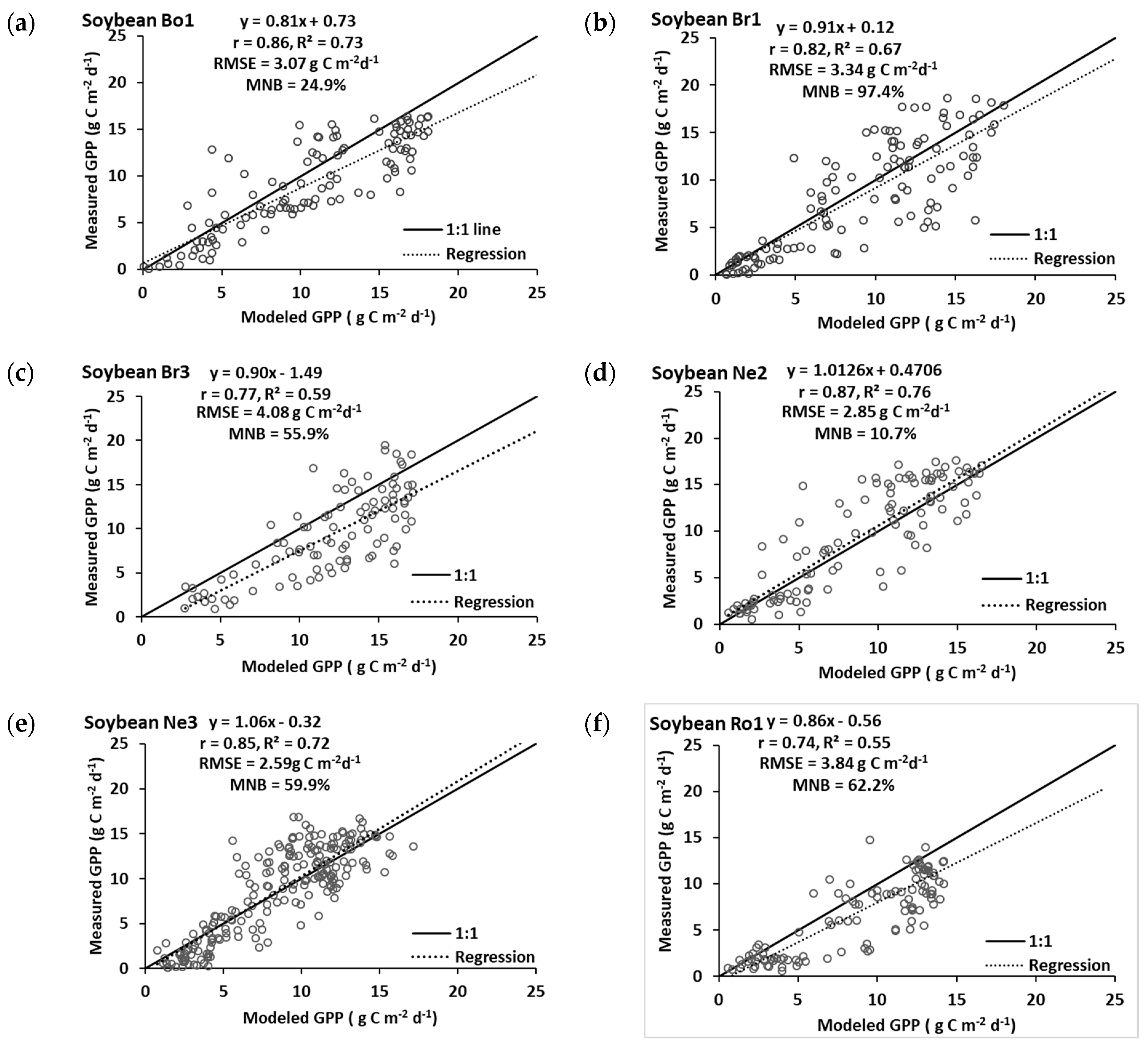
3.2. Maize and Soybean Field Years

While several sites were relatively unbiased (<15% MNB), the model tended to overestimate GPP overall. Most of the underestimation occurred at low GPP values (Figure 5 and Figure 6). Another trend is that the correlation between measured and modeled GPP values is stronger with maize than with soybean datasets (R² of 0.65–0.87 for maize and 0.55–0.75 for soybeans).

4. Discussion

This study utilized seven fields from four geographic locations. The agreement between modeled and measured values is not as strong as for maize and soybean GPP at sites in southeastern Nebraska alone in the original study [13] (overall slope of 0.94 ± 0.02, R² = 0.91, RMSE = 2.6 g C m⁻² d⁻¹, and MNB = 1.7%). Thus, the MNB of 30.5% across all sites in the current study is of concern (Figure 3a). It was expected that errors would be larger when using modeled input data as opposed to measured input data specific to the site. This was the case for Cui et al. [1], who attained an RMSE of 2.97 g C m⁻² d⁻¹ when comparing their modeled GPP data to in situ derived GPP of mixed land cover in the Heihe River Basin, China. Three of the seven fields, which include 36 of 65 total field years, are located in southeastern Nebraska and are the same as those used in the original study. With over half of the field years from this specific location, a calibration bias may have occurred. This bias may have led to smaller errors for the Nebraska sites and larger errors for the non-Nebraska sites than would be the case if the field years were more evenly represented for model calibration (Table 2).

In addition, there are inherent errors and uncertainties in the gridded Daymet data [29], attributed to weaker agreement between measured and modeled daily GPP values. Additionally, the gLAI algorithms used in this study were developed using the Mead, NE sites [20] and may not be ideal estimators of gLAI for the other sites due to characteristics not captured in the site-specific algorithms used in this study. Unfortunately, ground data were not available at the other AmeriFlux locations to generate more generic gLAI algorithms. The underestimation of early and late season GPP is attributed to the sensitivity of gLAI algorithms to soil background at low LAI and the inaccurate representation of canopy architecture with the given k constants when foliage density is low. In both cases, any noise in the approach is amplified due to low values of GPP during these periods.

The correlation between measured and modeled GPP values tended to be higher with maize than with soybean datasets (Figure 3b,c). The association among individual sites varied as well (Figure 5 and Figure 6). Factors contributing to a trend of a stronger association with the maize data include (1) the increased sensitivity to diffuse light of soybean plants compared to maize (β of 0.294 ± 0.002 for soybean, 0.181 ± 0.014 for maize) combined with the concerns regarding PARin data (discussed below); (2) estimates of gLAI may be a factor as gLAI algorithms for maize and soybean were developed for the Mead, NE training sites (US-Ne1, US-Ne2, and US-Ne3) and may not adequately estimate gLAI for the other locations which may have different plant densities (there is also uncertainty associated with separating green and nongreen leaf material during senescence [30]); (3) there were fewer soybean field years (17) than maize field years (30) with which to train the scalars, which may have allowed for more error in the soybean scalars due to the smaller sample size (Table 2); (4) the soybean growing season is much shorter than for maize, so there are fewer data points to calibrate/validate the model; (5) the temperature scalar was selected based on optimal temperatures for maize. There are physiological differences between C3 and C4 plants that may account for minor shifts in the optimal temperature range. However, using crop-specific temperature ranges will complicate the model and require in-season crop type maps. This would reduce the applicability of generating regional estimates.

To further understand errors in the GPP estimates, preliminary investigations were undertaken to determine the potential contribution of Daymet-derived values, scalars of the LUEc, and gLAI.

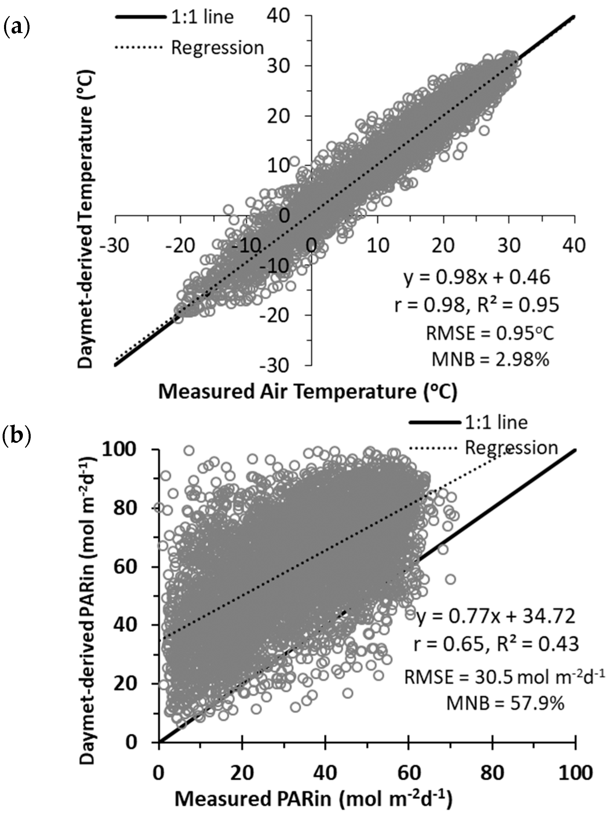
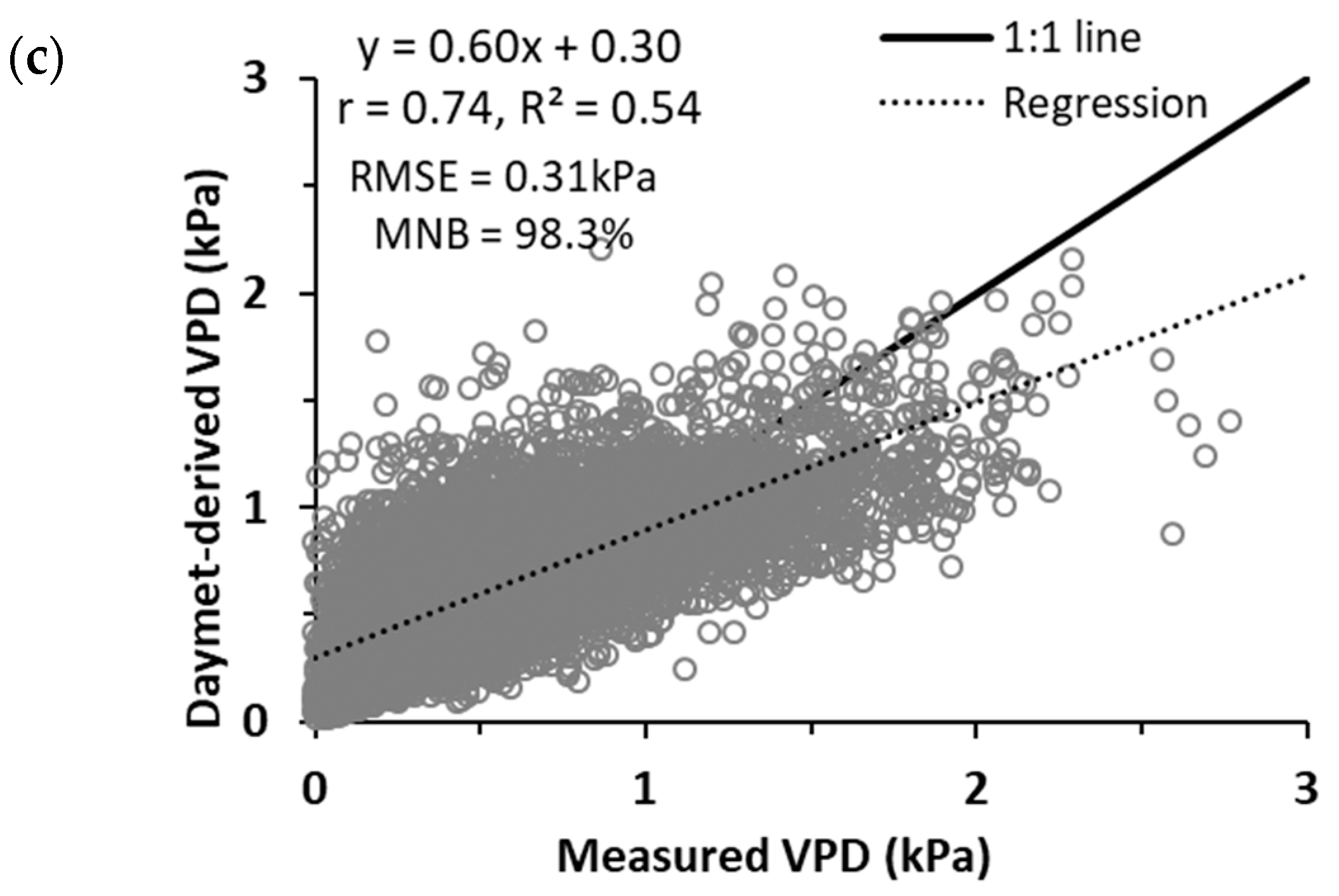
4.1. Daymet-Derived PARin and VPD

Daymet-derived values are compared to those measured at the AmeriFlux sites in Figure 7. T_ave values (Equation (1), using Daymet T_min and T_max) showed good agreement with AmeriFlux measurements (Figure 7a). Daily PARin values and VPD (Equation (2) using Daymet vapor pressure) were less consistent (R² of 0.48 and 0.54, respectively) (Figure 7b,c).

Overestimation of PARin (Figure 7b) would result in a decrease in the C_scalar value and is self-correcting in the calibration process which accounts for some of the differences in ε₀ and β (Table 4). By isolating PAR and LAI as variables for GPP modeling, Suyker and Verma [3] showed that PAR was a predominant factor in GPP variability. Gilabert et al. [31] employed an optimization scheme by adjusting values of PAR, the fraction of APAR, and ε (using the Monteith approach of Equation (9) with the product of the fraction of APAR and PAR equal to APAR). They found that PAR and the fraction of APAR were the most important factors in estimating daily GPP. The present study suggests an unsystematic error in PARin (and thus APAR) values. This unsystematic error in PARin is attributed to the Daymet calculation of shortwave radiation from which PARin is estimated (Equation (3)) and/or our attempt to upscale field-level PARin and GPP measurements to the Daymet 1 km grid. Overestimation of PARin will overestimate the amount of light available for photosynthesis in APAR calculations (Equation (10)) and reduce the model’s ability to properly account for contributions of diffuse light to GPP (Equation (11)). Other sources of input for PARin are likely needed [32,33].

Likewise, the apparent poor representation of the Daymet vapor pressure product for a specific site location and the fact that the inherent error is less predictable implies that a new source may be needed for this variable. One such source for both vapor pressure and PARin data could be PRISM (Parameter-elevation Relationships on Independent Slopes Model; PRISM [34]), which Mourtzinis et al. [29] found more accurate than Daymet. Underestimation of Daymet-derived VPD is likely due to the air mass over agricultural fields, especially irrigated agricultural fields, having lower VPD than reported for grids in which the fields are located. Underestimation of VPD increases the W_scalar value, which may inaccurately represent water stress conditions at field sites. Additionally, the calibration is influenced by 17 irrigated field years at the Mead, NE sites (US-Ne1 and US-Ne2; 58% of the field years used to calibrate the LUEc). This may have biased the σ_Wscalar parameter to better reflect irrigated crop management practices while the other five fields are under rainfed crop management. The modeled VPD would likely be overestimated at the two Mead, NE sites due to VPD being anthropogenically lowered through the irrigation practice. While the rainfed sites have higher annual precipitation rates than the Mead, NE sites, the timing is irregular and can contribute to greater uncertainty; irrigation at US-Ne1 and US-Ne2 supplements rainfall and thus reduces uncertainty. Thus, irrigation bias could increase error in modeled GPP at the rainfed sites.

4.2. LUEc Scalars

The scalars were generalized to better estimate GPP across the various sites within the region rather than calibrate scalars for each site, causing them to be less precise for any given location than those calculated for the Nebraska sites in the previous study [13]. The LUEc was run with all scalars set to a value of 1 to investigate their impact in the LUEc on the GPP calculation using the gridded datasets. GPP calculated with the scalars set to 1 had an RMSE of 5.35 g C m⁻² d⁻¹, an R² of 0.71, and an MNB value of 104.3% (Figure 8). Although the scalars may have been more effective if more accurate gridded input data were available, the model performed better overall with the scalars derived in this study using the Daymet and MODIS data than when run strictly as a LUE model. This supports the need to include meteorological data (stressors) in estimates of GPP, in contrast to an observation of Tramontana et al. [8] that predictions based on remotely sensed data gave optimally accurate estimates.

4.3. gLAI Estimates

LAI is a primary consideration in estimating net primary productivity [35]. The gLAI values used in this study were not verified at the non-Nebraska sites as no gLAI measurements are available for those sites. Thus relationships previously developed for the three Nebraska sites [13] were used. Of concern is the relationship with the gLAI after peak green-up. In addition to the fact that the algorithms were developed over a geographically limited area, the uncertainty associated with separating green and nongreen leaf material during senescence likely also contributed to less reliable gLAI estimates during senescence. Algorithms using a red edge band are less sensitive to nongreen leaf material [20]; however, the temporal resolution would have been reduced and increased uncertainty in interpolation had MERIS or Sentinel-2 data been selected.

4.4. APAR Importance in GPP Estimates

Overestimation of PARin greatly affects APAR in a manner that causes overestimation of GPP, which will inflate the MNB. Estimated APAR (Equation (10)) for the three Nebraska sites was plotted as a function of measured APAR in an attempt to determine how well the model was estimating the variable. Similar data were not available from the AmeriFlux website for the other sites. Two of the inputs in calculating APAR are gLAI and PARin, and a good portion of the increased error is attributed to the APAR term in the GPP equation (Equation (9)). When compared to measured APAR, estimated APAR for the three Nebraska sites (US-Ne1, US-Ne2, and US-Ne3) had a combined RMSE of 10.5 mol m⁻² d⁻¹, with an r of 0.72 and an R² of 0.53 (Figure 9a). When the data are separated into green-up (DOY ≤ 220) and post-green peak (DOY > 220) sets, it becomes apparent that there is a stronger correlation between measured and modeled APAR during the green-up phase than the post green-up phase (Figure 9b,c).

5. Conclusions

The main objective of this study was to evaluate the potential of the LUEc enhanced four-scalar light use efficiency approach of Nguy-Robertson et al. [13] to provide regional GPP estimates. By incorporating MODIS imagery and gridded weather data into the LUEc, daily GPP was estimated over the entire growing season in seven U.S. Corn Belt agricultural sites in four Midwestern US locations. Overall RMSE between measured GPP and modeled GPP for all field years was 3.5 g C m⁻² d⁻¹. This is an increase in RMSE of 0.9 g C m⁻² d⁻¹ compared to the in situ-based study [13]. However, the MNB of 30.5% is of particular concern. Generalized scalars were developed for maize and soybeans when the model was calibrated with remotely sensed derived gLAI data and gridded weather data from all seven sites. GPP estimates were better at some sites (Mead, NE) than at others. Accuracy of the LUEc estimates decreased when remotely sensed and gridded weather data inputs were used compared to the results of Nguy-Robertson et al. [13]. While accuracy decreased, so did the amount of resources required to run the model. The findings of this study indicate that the LUEc can provide acceptable daily GPP estimates for regions outside eastern Nebraska (for which the model was originally tested) using gridded and remotely sensed data. The LUEc performs better than a LUE model that does not incorporate stressors, supporting the need to include meteorological data (stressors) in estimating daily GPP. Future research should be conducted to determine if more generalized coefficients can be derived to allow the model to function accurately at broader regional scales.

References

1. Cui, T.; Wang, Y.; Sun, R.; Qiao, C.; Fan, W.; Jiang, G.; Hao, L.; Zhang, L. Estimating vegetation primary production in the heihe river basin of China with multi-source and multi-scale data. PLoS ONE 2016. [Google Scholar] [CrossRef] [PubMed] [Green Version]
2. Beer, C.; Reichstein, M.; Tomelleri, E.; Ciais, P.; Jung, M.; Carvalhais, N.; Rödenbeck, C.; Arain, M.A.; Baldocchi, D.; Bonan, G.B.; et al. Terrestrial gross carbon dioxide uptake: Global distribution and covariation with climate. Science 2010. [Google Scholar] [CrossRef] [PubMed] [Green Version]
3. Suyker, A.E.; Verma, S.B. Gross primary production and ecosystem respiration of irrigated and rainfed maize-soybean cropping systems over 8 years. Agric. For. Meteorol. 2012. [Google Scholar] [CrossRef] [Green Version]
4. Matsushita, B.; Tamura, M. Integrating remotely sensed data with an ecosystem model to estimate net primary productivity in East Asia. Remote Sens. Environ. 2002. [Google Scholar] [CrossRef]
5. Heinsch, F.; Reeves, M.; Votava, P.; Kang, S.; Cristina, M.; Zhao, M.; Glassy, J.; Jolly, W.; Loehman, R.; Bowker, C.F.; et al. User’s Guide GPP and NPP (MOD17A2/A3) Products NASA MODIS Land Algorithm. Version 2.0; University of Montana: Missoula, MT, USA, 2003. [Google Scholar]
6. Heinsch, F.A.; Zhao, M.; Running, S.W.; Kimball, J.S.; Nemani, R.R.; Davis, K.J.; Bolstad, P.V.; Cook, B.D.; Desai, A.R.; Ricciuto, D.M.; et al. Evaluation of remote sensing based terrestrial productivity from MODIS using regional tower eddy flux network observations. IEEE Trans. Geosci. Remote Sens. 2006. [Google Scholar] [CrossRef] [Green Version]
7. Xiao, X.; Hollinger, D.; Aber, J.; Goltz, M.; Davidson, E.A.; Zhang, Q.; Moore, B. Satellite-based modeling of gross primary production in an evergreen needleleaf forest. Remote Sens. Environ. 2004. [Google Scholar] [CrossRef]
8. Tramontana, G.; Ichii, K.; Camps-Valls, G.; Tomelleri, E.; Papale, D. Uncertainty analysis of gross primary production upscaling using Random Forests, remote sensing and eddy covariance data. Remote Sens. Environ. 2015. [Google Scholar] [CrossRef]
9. Zhang, Y.; Xiao, X.; Wu, X.; Zhou, S.; Zhang, G.; Qin, Y.; Dong, J. A global moderate resolution dataset of gross primary production of vegetation for 2000–2016. Sci. Data 2017. [Google Scholar] [CrossRef] [Green Version]
10. Yuan, W.; Cai, W.; Xia, J.; Chen, J.; Liu, S.; Dong, W.; Merbold, L.; Law, B.; Arain, A.; Beringer, J.; et al. Global comparison of light use efficiency models for simulating terrestrial vegetation gross primary production based on the LaThuile database. Agric. For. Meteorol. 2014. [Google Scholar] [CrossRef]
11. Zhang, Y.; Song, C.; Sun, G.; Band, L.E.; McNulty, S.; Noormets, A.; Zhang, Q.; Zhang, Z. Development of a coupled carbon and water model for estimating global gross primary productivity and evapotranspiration based on eddy flux and remote sensing data. Agric. For. Meteorol. 2016. [Google Scholar] [CrossRef] [Green Version]
12. Running, S.; Zhao, M. Daily GPP and Annual NPP (MOD17A2/A3) Products NASA Earth Observing System MODIS Land Algorithm. In MOD17 User’s Guide; 2015; Available online: https://www.ntsg.umt.edu/files/modis/MOD17UsersGuide2015_v3.pdf (accessed on 9 October 2020).
13. Nguy-Robertson, A.; Suyker, A.; Xiao, X. Modeling gross primary production of maize and soybean croplands using light quality, temperature, water stress, and phenology. Agric. For. Meteorol. 2015. [Google Scholar] [CrossRef] [Green Version]
14. Gitelson, A.A.; Arkebauer, T.J.; Suyker, A.E. Convergence of daily light use efficiency in irrigated and rainfed C3 and C4 crops. Remote Sens. Environ. 2018. [Google Scholar] [CrossRef]
15. Li, A.; Bian, J.; Lei, G.; Huang, C. Estimating the maximal light use efficiency for different vegetation through the CASA model combined with time-series remote sensing data and ground measurements. Remote Sens. 2012, 4, 3857–3876. [Google Scholar] [CrossRef] [Green Version]
16. Thornton, P.E.; Thornton, M.M.; Mayer, B.W.; Wilhelmi, N.; Wei, Y.; Devarakonda, R.; Cook, R.B. Daymet: Daily Surface Weather Data on a 1-km Grid for North America, Version 2; Data Set; Oak Ridge National Laboratory: Oak Ridge, TN, USA, 2014. [CrossRef]
17. Weiss, A.; Norman, J.M. Partitioning solar radiation into direct and diffuse, visible and near-infrared components. Agric. For. Meteorol. 1985. [Google Scholar] [CrossRef]
18. Biggs, W. Radiation Measurement. In Advanced Agricultural Instrumentation; Gensler, W.G., Ed.; Springer: Dordrecht, The Netherlands, 1986; pp. 3–20. ISBN 978-94-009-4404-6. [Google Scholar]
19. Gitelson, A.A. Wide Dynamic Range Vegetation Index for Remote Quantification of Biophysical Characteristics of Vegetation. J. Plant Physiol. 2004. [Google Scholar] [CrossRef] [PubMed] [Green Version]
20. Nguy-Robertson, A.L.; Gitelson, A.A. Algorithms for estimating green leaf area index in C3 and C4 crops for MODIS, Landsat TM/ETM+, MERIS, Sentinel MSI/OLCI, and Venμs sensors. Remote Sens. Lett. 2015. [Google Scholar] [CrossRef]
21. Monteith, J.L. Solar Radiation and Productivity in Tropical Ecosystems. J. Appl. Ecol. 1972. [Google Scholar] [CrossRef] [Green Version]
22. Raich, J.W. Potential net primary productivity in South America: Application of a global model. Ecol. Appl. 1991. [Google Scholar] [CrossRef] [Green Version]
23. Kalfas, J.L.; Xiao, X.; Vanegas, D.X.; Verma, S.B.; Suyker, A.E. Modeling gross primary production of irrigated and rain-fed maize using MODIS imagery and CO2 flux tower data. Agric. For. Meteorol. 2011. [Google Scholar] [CrossRef] [Green Version]
24. Wu, W.X.; Wang, S.Q.; Xiao, X.M.; Yu, G.R.; Fu, Y.L.; Hao, Y. Bin Modeling gross primary production of a temperate grassland ecosystem in Inner Mongolia, China, using MODIS imagery and climate data. Sci. China Ser. D Earth Sci. 2008. [Google Scholar] [CrossRef]
25. Maselli, F.; Papale, D.; Puletti, N.; Chirici, G.; Corona, P. Combining remote sensing and ancillary data to monitor the gross productivity of water-limited forest ecosystems. Remote Sens. Environ. 2009. [Google Scholar] [CrossRef] [Green Version]
26. Gilmanov, T.G.; Wylie, B.K.; Tieszen, L.L.; Meyers, T.P.; Baron, V.S.; Bernacchi, C.J.; Billesbach, D.P.; Burba, G.G.; Fischer, M.L.; Glenn, A.J.; et al. CO2 uptake and ecophysiological parameters of the grain crops of midcontinent North America: Estimates from flux tower measurements. Agric. Ecosyst. Environ. 2013. [Google Scholar] [CrossRef] [Green Version]
27. Reich, P.B.; Walters, M.B.; Ellsworth, D.S. Leaf age and season influence the relationships between leaf nitrogen, leaf mass per area and photosynthesis in maple and oak trees. Plant Cell Environ. 1991. [Google Scholar] [CrossRef]
28. Field, C.; Mooney, H.A. Leaf age and seasonal effects on light, water, and nitrogen use efficiency in a California shrub. Oecologia 1983. [Google Scholar] [CrossRef]
29. Mourtzinis, S.; Rattalino Edreira, J.I.; Conley, S.P.; Grassini, P. From grid to field: Assessing quality of gridded weather data for agricultural applications. Eur. J. Agron. 2017. [Google Scholar] [CrossRef] [Green Version]
30. Nguy-Robertson, A.; Peng, Y.; Arkebauer, T.; Scoby, D.; Schepers, J.; Gitelson, A. Using a Simple Leaf Color Chart to Estimate Leaf and Canopy Chlorophyll a Content in Maize (Zea mays). Commun. Soil Sci. Plant Anal. 2015. [Google Scholar] [CrossRef]
31. Gilabert, M.A.; Moreno, A.; Maselli, F.; Martínez, B.; Chiesi, M.; Sánchez-Ruiz, S.; García-Haro, F.J.; Pérez-Hoyos, A.; Campos-Taberner, M.; Pérez-Priego, O.; et al. Daily GPP estimates in Mediterranean ecosystems by combining remote sensing and meteorological data. ISPRS J. Photogramm. Remote Sens. 2015, 102, 184–197. [Google Scholar] [CrossRef]
32. Nasahara, K.N. Simple algorithm for estimation of photosynthetically active radiation (PAR) using satellite data. Sci. Online Lett. Atmos. 2009. [Google Scholar] [CrossRef] [Green Version]
33. Sakamoto, T.; Gitelson, A.A.; Wardlow, B.D.; Verma, S.B.; Suyker, A.E. Estimating daily gross primary production of maize based only on MODIS WDRVI and shortwave radiation data. Remote Sens. Environ. 2011. [Google Scholar] [CrossRef]
34. Daly, C.; Halbleib, M.; Smith, J.I.; Gibson, W.P.; Doggett, M.K.; Taylor, G.H.; Curtis, J.; Pasteris, P.P. Physiographically sensitive mapping of climatological temperature and precipitation across the conterminous United States. Int. J. Climatol. 2008, 28, 2031–2064. [Google Scholar] [CrossRef]
35. Hazarika, M.K.; Yasuoka, Y.; Ito, A.; Dye, D. Estimation of net primary productivity by integrating remote sensing data with an ecosystem model. Remote Sens. Environ. 2005. [Google Scholar] [CrossRef]
Figure 1. Map indicating the locations of the seven agricultural AmeriFlux sites in the U.S. Midwest used in this study.
Remotesensing 12 03956 g001
Figure 2. Climographs from cities near the AmeriFlux sites. US-Ne1, US-Ne2, and US-Ne3 are located at the University of Nebraska’s Eastern Nebraska Research and Extension Center near Mead, NE; US-Br1 and US-Br2 located approximately 8 km southwest of Ames, Iowa; US-Bo1 is located approximately 12 km south of Champaign, Illinois and US-Ro1 is located near Rosemount, Minnesota which is located approximately 24 km south of Saint Paul, Minnesota. (Source: 1981–2010 normals, usclimatedata.com).
Remotesensing 12 03956 g002
Figure 3. The relationship between AmeriFlux measured and LUEc modeled GPP for (a) all validation data with slope confidence interval ± 0.02 (n = 2130), (b) all maize validation data with slope confidence interval ± 0.02 (n = 1379), and (c) all soybean validation data with slope confidence interval ± 0.05 (n = 751).
Remotesensing 12 03956 g003aRemotesensing 12 03956 g003b
Figure 4. AmeriFlux measured GPP yearly total vs. LUEc modeled GPP yearly totals for every validation field year.
Remotesensing 12 03956 g004
Figure 5. Measured AmeriFlux vs. LUEc modeled daily GPP for all maize validation years by site: (a) US-Bo1; (b) US-Br1; (c) US-Br3; (d) UN-Ne1; (e) US-Ne2; (f) US-Ne3; and (g) US-Ro1.
Remotesensing 12 03956 g005
Figure 6. Measured AmeriFlux vs. LUEc modeled daily GPP for all soybean validation years by site: (a) US-Bo1; (b) US-Br1; (c) US-Br3; (d) US-Ne2; (e) US-Ne3; and (f) US-Ro1.
Remotesensing 12 03956 g006
Figure 7. Daymet-derived daily values as functions of AmeriFlux measured values for (a) average daily temperature, (b) PARin, and (c) vapor pressure deficit (VPD).
Remotesensing 12 03956 g007aRemotesensing 12 03956 g007b
Figure 8. AmeriFlux measured GPP plotted as a function of LUEc modeled GPP when (a) all scalar values are used; (b) all scalar values are set to 1 and the model is run as a pure LUE model with the scalars completely negated.
Remotesensing 12 03956 g008
Figure 9. AmeriFlux measured APAR as a function of Daymet and MODIS derived APAR for all three Nebraska sites for (a) all growing season days, (b) all green-up days, (c) all post green peak days.
Remotesensing 12 03956 g009