1. Introduction
Power lines are a typical part of urban and rural landscapes. Due to the need for power, national and regional networks cover most of the world and continue to expand. They require regular monitoring and maintenance work. Monitoring power lines features two aspects: power line components and occlusions of the line corridor. Both are important and interconnected and are thus often addressed simultaneously.
The power line corridor is a 3D buffer around the wires and is defined by the set distance from the wires. It is thus necessary to find the precise position of the wires [
1]. Regular inspections of vegetation inside and near the power line corridor are needed to identify trees or branches that need to be cut due to safety concerns, as the direct proximity of trees in a line corridor might trigger, for example, a bushfire. There are monitoring methods that are used to identify branches or canopies that endanger the inviolability of the power line corridor [
2] or detect and classify trees to help evaluate the impact on the line [
3]. Other techniques focus on volumetric analysis in order to evaluate the impact of the vegetation and its progression by calculating a differential map of a digital surface model (DSM) for two epochs [
4].
A range of techniques have been implemented to solve the above problem. They vary from mundane and time-consuming methods of classical surveying to technologically advanced and highly expensive ones. Among the most popular inventory methods for inspecting power lines are airborne laser scanning [
5,
6,
7,
8] and mobile terrestrial scanning [
9,
10]. The dense point clouds generated by laser scanning can be used to form models of 3D power lines, in the context of surrounding vegetation, and a survey network. The typical workflow features classifying point clouds, creating the digital terrain model (DTM), and 3D line modeling [
11]. Algorithms based on point position, the intensity of response, multiple echoes, and 2D projections enable automated data processing [
6,
12,
13]. Although Light Detection and Ranging (LiDAR) is an effective and robust method, it has some drawbacks. Some, such as problems with suitable weather conditions, are partially shared with passive methods. Additional drawbacks include problems with identifying towers and simply the cost of the equipment, survey, and processing [
14]. Some research has also dealt with a combination of unmanned aerial vehicle (UAV) technology and LiDAR for surveying power lines [
5,
15,
16]. The availability of lighter LiDAR scanners and developments in the UAV platforms have contributed to improving efficiency. Although this technology has potential for further development, the cost of a device in combination with the high risk of failure decreases its economic efficiency.
Many applications use optical images and computer vision systems [
17]. Satellite, airborne, and UAV images have been employed [
18,
19]. Satellite images, owing to their low resolution, are limited to providing generalized information on terrains and vegetation [
20]. Aerial images rely significantly on manual stereo measurements [
19]. UAV-based optical images can provide accurate and high-resolution data [
21], and their use with a range of stereomatching algorithms is a promising solution. Attempts have been made to consider photogrammetry as a source of the point cloud and to analyze and filter data similarly to the procedure in LiDAR [
22]. Automatic software for dense matching, where the geometry of power lines is reconstructed, could be a fast and convenient solution. In addition to its clear drawbacks relating to optical images, such as the sensitivity to changes in lighting conditions, and the atmospheric influence, the radiometric differences between lines and a background make it even less effective. The lines usually occupy a small part of a photo; otherwise, the time needed for the surveying, the size of the survey data, and the processing time increase. Furthermore, the complexity and the variability of the background is an obstacle for the 3D line reconstruction [
23]. The aforementioned reasons and the use of the outliers’ approach might preclude the operation of dense matching algorithms. For these reasons, this solution is not feasible.
Other solutions have been proposed for clearance monitoring using aerial images, but methods that use UAVs as the main source of data are becoming increasingly popular. The biggest advantages to using UAVs are their low altitude of flight and the flexibility and economy of the method in comparison with airborne photogrammetry [
24,
25]. Both multi-rotors and fixed wings are used for this task. The former constructions are especially useful for precise surveys at a low altitude, but the latter approaches are more efficient and have a greater fly range [
18].
Considerable research has been dedicated to power line monitoring using UAVs. Most of it has focused solely on wire detection in images [
26,
27,
28,
29,
30,
31,
32,
33,
34], but a few studies have taken a more holistic approach by considering not only the position of the power line, but also the line corridor and obstacles. The means of data processing and 3D power line reconstruction are different and depend on the aim of the calculation. Such an approach was proposed in two papers [
26,
35]. One focused on dense matching algorithms and the automation of obstacle detection, whereas power line reconstruction was performed manually, and aided by epipolar images [
23]. The other study implemented the results of past work together with fully automated line detection algorithms based on images [
35]. This method is based on changes in the gradient combined with the high gray response of the power line and assumes multiple thresholds. This solution provides good results, although it has yet to be proven to work with more versatile data. Similarly, research on epipolar imagery was presented in another piece of research [
36], where a real-time system was developed for obstacle avoidance by UAVs as they monitored power lines. To calculate the relative 3D position of the power lines, several steps were implemented, including TopHat transform and the cross-based arbitrary shape support region method, to create a depth map. The study assumed that the background was not complex, and featured either the sky or some treetops. Another holistic approach used semantic segmentation based on fully convolutional neural networks to enhance depth maps and accurately reconstruct linear objects [
37]. The research also used enhanced dense matching to detect obstacles in the power line corridor. The neural networks were also used successfully for line segmentation in another study [
38]. The effectiveness of these algorithms is at least 80%. However, their major drawback is the demand for a vast learning dataset [
3]. Additionally, there are hardly any cases of a comprehensive methodology for detecting and reconstructing power lines in the literature using neural networks [
39]. Additional research on the 3D reconstruction of power lines was presented in two papers by the same authors [
40,
41]. In both, the lines are initially detected from epipolar images using a simple extraction template. Three-dimensional reconstruction is performed differently in each, however. One introduces a 3D grid based on the expected ground sampling distance (GSD) and the positions of the utility poles [
40]. The grid is then reprojected on images to validate the detected power lines and establish their relative correspondence. In the second paper, all combinations of wires detected in both images in a stereopair are considered and then reprojected on a third image to validate the choice [
41].
This paper aims to develop a comprehensive and robust method for occlusion monitoring in the power line corridor (
Figure 1). The main goals are to minimize the time needed to perform the survey and the user input in subsequent processing. The same dataset was thus used to reconstruct power lines and acquire a point cloud representation of a DSM for a possible occlusion check. However, images suitable for the creation of a dense point cloud representation of the terrain usually record power lines as barely distinguishable objects that are only a few pixels wide. Therefore, additional processing is required to successfully extract and model power lines.
The remainder of this paper is structured as follows:
Section 2 describes the proposed method, including the data acquisition process, initial data processing, 2D image processing, 3D reconstruction of power lines, and obstacle detection. The datasets acquired to create and test the proposed method are also presented in
Section 2.
Section 3 describes the results of UAV image processing along with the assessment of their accuracy. A discussion of errors and their possible sources is in
Section 4.
Section 5 offers the conclusions of this paper. In
Appendix A, the additional results of a threshold sensitivity analysis are included.
2. Materials and Methods
The proposed method features the following steps (
Figure 2):
Data acquisition—the terrain was imaged according to certain principles of photogrammetry to ensure high accuracy and automated processing.
Bundle adjustment and data ordering—the image data were processed using photogrammetric software to estimate the exterior orientation elements (EOE) and the interior orientation elements (IOE) for DSM reconstruction. The data were then ordered into consecutive stereopairs.
Power line detection in images and reconstruction of 3D geometry—the process uses several techniques, both on separate images (2D) as well as stereopairs (3D). The approximate position of each power line was calculated, either from manual input or 3D points projected on the image. The images were then processed using the modified Prewitt operator, automatic thresholding, and binarization. The random sample consensus (RANSAC) algorithm with additional parameters was then used to calculate the adjusted position of the detected power line. Three-dimensional reconstruction was then performed using the detected power lines and principles of epipolar geometry.
Detection of obstacles within the power line corridor—a simple procedure where the distance between reconstructed power lines and the point cloud representation of DSM is computed; occluding points are then bound into voxels [
37] and clustered into objects [
42].
All the steps are described in detail below.
2.1. Data Acquisition
Appropriate data acquisition can enable the detection of power lines and is as important as the methods for the subsequent processing of the data. Some requirements need to be satisfied to ensure the reliable operation of the algorithm. While maintaining the highest efficiency, the measurement requirements of the data should be universal enough to allow for the use of different cameras and UAVs.
First, it is important to define image quality requirements. In this case, the most significant parameter is resolution as defined by the GSD. The maximal GSD to ensure that the wires are detected must be smaller than their diameters. However, to increase the efficiency of detection, the GSD should be half the diameter. Another important aspect is the camera’s exposure settings, which must ensure that the wires can be distinguished from the background (
Table 1). Owing to the small size of the wires, the ISO setting should be as small as possible. To avoid blurred images, the shutter speed should be adjusted to UAV flight speed, and should not be higher than the ratio of the GSD to the speed of the UAV. If the camera settings allow for the disabling of the low-pass filter, this should be done. Moreover, for the high accuracy of the end product, the use of a global shutter camera would be advised.
Secondly, data acquisition must ensure an appropriate data structure for the algorithm. Because a major function of the algorithm is to transfer detection between stereopairs, the flight plan has to ensure the visibility of the wires for all subsequent images between poles. To meet this requirement, the flight path must be linear, parallel to the power line, and consist of at least two rows, placed on opposite sides of the surveyed corridor (
Figure 3). Another advantage of a linear flight plan is the possibility of measuring power lines over distances ranging from a few (multi-rotor) to dozens of kilometers (fixed wing) in one flight.
Third, image overlap and the field of view should be carefully planned. The side overlap should allow for the wires to be visible in both neighboring strips. The front overlap should not be lower than 50% (at the height of the wires, overlap on the ground is higher) to ensure the correct transfer of detection between stereopairs, but this should also not exceed the minimum duration of the acquisition of the camera. The front overlap should thus be adjusted according to flight speed and altitude.
The last thing to take into consideration while planning a survey is the global accuracy of the resultant product. Photogrammetric blocks, in the case of corridor mapping, have highly unstable geometry. To maintain high accuracy and prevent errors that could occur in self-calibration due to potentially high correlation between interior and exterior camera orientation, additional measures have to be introduced. A network of ground control points (GCPs) can be introduced to stabilize the block [
43]. However, it might not be feasible in remote terrains and it also increases the time and cost of the survey. Equipping the UAV with a global navigation satellite system (GNSS) post-processing kinematic (PPK) receiver to achieve centimeter accuracy of EOE can also help to mitigate the problem [
44]. However, the PPK receiver increases the overall cost of the platform. To ensure correct results, one of those measures must be introduced.
2.2. Bundle Adjustment and Data Ordering
The Agisoft Metashape Professional (version 1.6.0 build 9128) software was used to estimate both the IOE and EOE for the obtained UAV images. All images collected during the mission were processed together. The processing, which included automatic bundle adjustment with self-calibration, was mostly automated. A typical set of parameters were estimated during self-calibration [
45], utilizing the Brown distortion model [
46]:
principal point position: x0, y0,
focal length: f,
parameters of radial distortion: r1, r2, r3,
parameters of tangential distortion: p1, p2.
The global accuracy was ensured either by the use of GCPs or precise EOE (GNSS PPK processing). Ultimately, the resulting data contained undistorted images (achieved using the calculated parameters of calibration), along with their corresponding EOE and calibrated focal length.
The data ordering process, as shown in
Figure 4, involved firstly automatically assigning the images to flight lines (strip) and then subsequently assigning stereopairs, consisting of the two closest images from their opposite strips (
Figure 3), which were subjected to further processing. A set of ordered stereopairs is crucial for the seamless operation of the algorithm. It was necessary to process the images in a defined order (in the direction of processing). Therefore, stereopairs were selected and sorted in ascending order in the direction of processing. This direction was defined by the ordered coordinates of the poles acquired through Agisoft Metashape (or obtained from the operator of the power line).
For the seamless operation of the algorithm, a power line fragment targeted in a UAV flight survey mission was divided into survey sections that were subjected to further processing. The section was defined by a starting utility pole, transfer utility poles, and an ending utility pole. One survey section might have consisted of several power line spans (
Figure 5). The order of the poles in the survey section determined the direction of subsequent image processing, and thus had a crucial effect on the entire process of power line detection.
Defining the survey sections for image processing was an important stage in data ordering. Depending on the type of power line, they were defined differently. For high-voltage lines, one span was defined as one survey section. For medium-voltage lines, the survey section included rectilinear sections of the power line. To divide the survey section, each image containing a pole was analyzed. Three-dimensional lines connecting a pole, captured within the image, and its neighbors were reprojected on the image. When the in-line direction change was greater than 1°, the pole, captured within the image, was assumed to mark the end of the given survey section and the start of a new one. Data thus prepared and ordered were then subjected to further processing.
2.3. Power Line Detection in Images
Detection and reconstruction were performed separately, using dedicated algorithms. The process consists of multiple subsequent steps and was written in the Python programming language.
For effective automation, it was necessary to detect the power lines continuously through a sequence of images. The simplest and most accurate way to transfer detection between neighboring photographs is through 3D space, where the relevant geometry was reconstructed and then projected onto the next image. Such reconstruction was possible by using two across-track neighboring images. Thus, the processing unit in the detection algorithm was a single stereopair. Detection was then performed separately on both images while keeping track of the respective wires. Both images were then used to reconstruct the 3D position of the given power line.
The process can be divided into several steps (
Figure 6) that vary depending on the processed image: detection (Case 1—images capturing the survey sections from the starting utility pole) or continued detection (Case 2—all remaining images).
Due to the wire’s relative position in the image and its sag, the wire was almost never recorded as a straight line in an image. The discrepancies between the fitted line and the empirically captured position of each wire varied from two to dozens of pixels. Moreover, due to varying backgrounds, neither the color of the wire nor the contrast in the image remained constant. To accommodate change in both position and contrast, a local, constantly adapting approach was chosen. For each wire, the image was divided into small, ordered sections within which the power line could be approximated by a straight line. To define the position and order of the processing windows, past information about the approximate positions and directions of the power lines was needed. This was acquired either by a manual initialization procedure in the image at the beginning of the survey section or by using projected points from the preceding stereopair.
2.3.1. Approximation of Position and Direction of Power Line
To approximate the position and direction of each power line, two approaches were adopted according to the given case.
Case 1—starting detection required a manual input in the form of two points per power line in the image. This was sufficient to calculate the general direction and position of the given wire, and important information was obtained regarding the correspondence of the wires between image stereopairs. Owing to the different modes of construction of the utility poles, the wires could be captured in different orders between images.
To transfer detection between images (Case 2), the 3D coordinates of the power lines were used and were then projected onto images in the subsequent stereopair. The line was fitted to points that were within the boundaries of the image. The line parameters defined sought after the position and direction of the power line.
2.3.2. Initial Image Processing and Edge Detection
To detect power lines in images, a method to enhance their visibility was needed. For this purpose, a decorrelation stretch of histograms of the images was used [
47]. The enhancement algorithm was based on principal component analysis (PCA). The covariance matrix was calculated from the three RGB bands, and its eigenvalues were found to form coefficients of the transformation of the principal component. After the normalization of the transform bands, new image bands were created. The result was compared with the weighted arithmetic mean of all bands (
Figure 7) [
48]. The third band of the processed image was chosen as it delivered the highest visibility of the power line.
The edge detection operator needed to be set to enhance long, linear edges, and presumably only ones that aligned with the approximated direction of the power line. The modified Prewitt operator was used for this. The operator was expanded from its base 3 × 3 form to 31 × 31. Then, the rotation to the direction of the power line was computed using the previously acquired approximate parameters of the power line. The final operator scheme is shown in
Figure 8.
The convolution of the grayscale image was calculated using the modified Prewitt operator. The resulting image was not normalized and had both negative and positive values.
All the highest values occurred along the edges on the right side, and all the lowest values occurred along the edges on the left side. Two images were created: one to identify edges on the right side and the other to identify those on the left side. Both images were then normalized to eight-bit unsigned integer space and subsequently binarized (
Figure 9).
2.3.3. Power Line Detection
Separately, for each wire in the image, the process of detection was conducted over small image segments. The position and order of the segments were calculated according to the approximated position and direction of the wire, and they were evenly spaced, with at least a 10% overlap, along the line between the captured utility pole (if present) and the boundary of the image (
Figure 10). The order of the segments was set along the direction of the power line.
For each segment, the detection was performed as follows. In images of both the left and the right edges, a line was fitted within the data using the RANSAC algorithm [
49]. Then, detected symmetric lines were used to determine the final position of the power line. A list of parameters of detection was provided, together with the results, to assess the correctness of the process:
—right edge coherence, a quotient of inliers in RANSAC to all positive pixels in the image segment;
—left edge coherence, a quotient of inliers in RANSAC to all positive pixels in the image segment;
—the maximum distance between lines of the right and left edges within the image segment;
—parallelism coefficient, the quotient of the minimal and maximum distances between lines of the right and left edges within the image segment.
Depending on the values of the above parameters, the detection was judged to be successful or incorrect/implausible. If the detection was accepted, the parameters of the line were calculated for the line between the right and left images, and involved the following:
image coordinates of both ends of the detected line segment,
a, b parameters of line equation y = ax + b.
The rejected detection was replaced by an extension of parameters detected in the previous image segment. The process was repeated until the end of the image was reached. All parameters of the line for all segments were then saved for further processing.
2.3.4. Three-Dimensional Geometry Reconstruction
The last stage of the power line detection process was 3D geometry reconstruction. The global coordinates of the points along the power line were determined using the spatial intersection of homologous rays. The problem was to identify homologous points on wires between the left and the right images in a given stereopair. Previous knowledge of corresponding wires and epipolar geometry was invoked to perform this task. Instead of identifying corresponding points on wires using feature descriptors, a purely geometric approach was chosen.
Each wire captured within the left and right images in a stereopair was represented by line segments established in the detection step. Two hundred evenly spaced points were chosen along the wire on the left image. Their coordinates were derived directly from the parameters of segments of the line. Then, for the nodal points, the respective epipolar lines on the right image were computed (
Figure 11a) using a fundamental matrix (Equation (1)):
where:
x′ = [x y 1]—focal coordinates of a point on the left image,
F—fundamental matrix, calculated from the positions and rotations of the left and right images,
k″ = [A B C]—parameters of line equation in a general form.
The intersections of the epipolar lines and line segments representing the wire on the right image were then calculated to determine key points in it. Finally, the corresponding key points in both images were used to compute the spatial intersections and determine the terrain 3D coordinates (
Figure 11b). Together, they provided a discrete representation of the wire.
2.3.5. Catenary Curve Fitting
The wire in discrete representation was not sufficient for assessing power line diagnostics. The sag of the wire, which is acquired from a fitted catenary curve, was also needed. The expression for it describes the geometry of a wire hanging under its weight when supported only at its ends:
where:
—the catenary constant, where
—horizontal force on the cable [kG/mm2],
q—the weight of the cable per unit arclength [kG/(m·mm2)].
The catenary curve was fitted to previously obtained points representing the wires using the classical approach. It assumes that the points are represented in the local coordinate system, where the
x-axis runs along the wire, while the coordinates of the
y-axis correspond to the height of points on the wire. This coordinate system was defined independently for each wire, and the catenary equation was determined in the following form:
where:
The solution to Equation (3) was obtained by using the least squares method. Three randomly selected points from a set of representative points on the wire were used to calculate the approximate values of the unknowns (i.e.,
w0,
u0, and
k0). Together with the
x coordinate of each point, they were used to calculate the deviations in the
y coordinates and, subsequently, the adjusted parameters of the catenary curve that best fitted a series of data points. Using this, the maximum value of the sag of the wire was calculated as follows:
where:
,
, , and
—coordinates of the beginning and end of a catenary curve in the local coordinate system.
Owing to the large number of points representing each wire and the random nature of their selection to calculate approximate values of parameters of the catenary curve, unsatisfactory results of curve fitting were possible (
Figure 12a). To avoid such errors and obtain the best possible result, two additional assumptions were introduced: only solutions where the value of the sag of the wire (Equation (4)) was positive were considered, and the choice of the best solution was based on the RANSAC algorithm (
Figure 12b).
The final curve parameters and discrete representation of the wire were saved. The latter consisted of 1000 equally spaced points along each curve per wire.
2.4. Detection of Obstacles within the Power Line Corridor
One objective of the 3D reconstruction of power lines and the creation of the DSM is to monitor the separation of the wires from elements of land cover. We had to check whether the UAV-derived data allowed for the correct identification of obstacles too close to the power lines.
The purpose of the analysis here was to detect DSM fragments (points in the point cloud) that were within the power line corridor. Cloud Compare software and its cloud-to-cloud distance function were used for this task. For each point in the point cloud constituting the DSM, the spatial distance to the nearest point representing the wire was determined.
Next, all the points recorded within the corridor distance were segmented into set size voxels (3D pixels) and subsequently clustered into objects using neighborhood connections. Objects consisting of only one voxel were removed from the dataset. For each object, its volume, center, and bounding box were recorded for further analysis by the power line operator (
Figure 13).
2.5. Verification and Quality Assessment
To assess the algorithm, three approaches were adopted. First, the quality of the power line detection and subsequent reconstruction was evaluated. All data used in this assessment were firstly processed and subsequently manually checked for correct and incorrect detection. All errors were marked, and a presumed source of error was noted.
Secondly, the global accuracy of the reconstruction of the power lines was compared to established methods—total station (TS) and terrestrial laser scanning (TLS). The comparison was conducted in three ways. For each wire, both horizontal and vertical position discrepancies were calculated. Additionally, sag values were compared between proposed and reference methods. Though TS and TLS accuracy capabilities reach millimeter levels, this is not the case for a highly dynamic object, where small environmental influences change its geometry. Wire sag changes substantially with a change in temperature, while wind gusts cause oscillating vibrations. Considering the time needed to carry out both TS and TLS surveys, one has to expect significant changes within the surveyed power line. This notably diminishes the accuracy of both methods. Thus, the data were not treated as ground truths, but as reference, comparison data. Thirdly, corridor occlusions detected using the proposed method and TLS data were compared.
2.6. Experimental Data
To conduct the assessment, data were collected for several fragments of medium- and high-voltage power lines. The power lines were located in Małopolskie Voivodeship (Poland), in areas with varied relief.
The data were divided into four datasets denoted as Dataset I, Dataset II, Dataset III, and Dataset IV. Dataset I was used to develop and optimize the algorithm. The effectiveness and the feasibility of the algorithm were analyzed on an independent dataset (Dataset II). The accuracy of the measurements of the power lines and corridor obstacle detection were assessed on Datasets III and IV. The datasets were independent, and therefore assessments of the reliability and accuracy of the proposed method were reliable.
2.6.1. Datasets I and II
Dataset I was used for threshold sensitivity analysis and algorithmic optimization. The survey area contained 13 middle-voltage power line spans (14 utility poles (
Figure 14a)), over 1.2 km in a rather flat area. The photogrammetric data were collected in March 2017 using a GRYF octocopter (FlyTech UAV, Krakow, Poland), fitted with a precision positioning system based on a single-frequency GNSS receiver Emlid Reach M+ (
Table 2). Dataset I contained 225 images captured with an a6000 camera (Sony, Tokyo, Japan) (
Table 3) and Nakton 40 mm (Voigtlander, Braunschweig, Germany). The flight was fully autonomous and was conducted linearly along the power line in two strips. The flight altitude was 60 m above ground level and 50 m above the top of the poles, which yielded 6 and 5 mm of GSD, respectively (
Table 4).
Dataset II was used to validate the feasibility, reliability, and efficiency of the proposed method. It consisted of 238 images captured with an a6000 camera (Sony) (
Table 3) and 30 mm Sigma lens (Sigma Corporation, Kawasaki, Japan) in November 2017. The flight was performed using a GRYF octocopter (FlyTech UAV). It was fully autonomous and was conducted in three strips parallel to the power line. The flight altitude was 70 m above ground and 40 m above the top of the poles (
Table 4). Both the side and front overlap between the images were 75%. The flight area covered four spans of high-voltage power lines (five utility poles (
Figure 14b)) with a total length of 1.4 km. Only two outer strips were used in the processing.
2.6.2. Datasets III and IV
Datasets III and IV were used to verify the accuracy of the proposed method. They included UAV imagery as well as the results of the survey of power lines through TLS and classic TS measurements. The 3D geometry of the wires is constantly changing as a consequence of changing weather conditions (especially changes in temperature). It was thus assumed that the data for the power lines needed to be collected using different methods simultaneously. Unfortunately, the time needed to perform each of the surveys varied greatly from a couple of hours (UAV) to a couple of days (TLS).
The data marked as Datasets III and IV concern power lines located in hilly and difficult to access areas. Dataset III contained data on a segment of a medium-voltage power line consisting of 10 spans, with a total length of 1.3 km. The segment was located in an area with a maximum height difference of 60 m. The power line was fitted with three transmission wires set at the same height. A 400 kV high-voltage power line was another object of research, and data related to it were collected in Dataset IV. The tested section of the power line with a total length of 1.55 km consisted of four spans. The height difference between the beginning and end of the analyzed power line section was 100 m, with a height difference of 60 m for one of the spans. It was fitted with 12 transmission wires and two ground wires, all positioned at varying heights.
The photogrammetric data in Datasets III and IV included high-resolution digital images of the power lines taken with a DSC-RX1RM2 (35 mm) non-metric camera (Sony) (
Table 3) from the GRYF octocopter (FlyTech UAV) on 6 December 2018 (
Table 4). The images were captured in two strips parallel to the power line that was the subject of the measurement. A network of GCPs and checkpoints (CPs) was established for each dataset. The coordinates of markers were determined by the GNSS real time network (RTN) method with a Leica GS16 receiver (Leica Geosystems AG, Sankt Gallen, Switzerland) that had a horizontal accuracy of 3 cm and a vertical accuracy of 5 cm.
The segments of power lines represented by Datasets III and IV were measured using other methods such as TLS and TS measurements for reference. Fieldwork was performed on 1–3 and 6 December 2018. The weather conditions during the measurements were variable. The temperature was between −5 °C and +5 °C, consequently changing the power line sag. In addition, on 2 and 3 December, the wind blew at a speed of up to 15 m/s (gusts), which caused the oscillating movement of the wires.
For TS measurements, a Nova MS50 (Leica Geosystems AG) was used. Each span (all its wires) was measured from a single instrument station approximately located in the middle of the span. A single wire point at its beginning and end, and several points along its entire length, were measured. The coordinates of the stations and reference points were determined by the GNSS RTN method. Using these data, the spatial coordinates of points representing the individual wires were determined.
In addition to the TS measurements, the power lines were measured using TLS. The Leica ScanStation C10 laser scanner (Leica Geosystems AG), together with a set of HDS (High Definition Survey) 6″ targets (Leica Geosystems AG), were used for this purpose. The TLS measurements were carried out using the three-tripod method with a traverse workflow. The resolutions of the TLS were 10 and 7.5 mm at a distance of 10 m. This was connected with the maximum reduction in measurement time while maintaining satisfactory scanning results and was preceded by tests to determine the optimum scanning resolution depending on the type of power line and the distance between stations. The data were collected at 39 stations for Dataset III and 29 stations for Dataset IV. Finally, the point clouds from all scanner stations were registered and georeferenced (
Figure 15) using Leica Cyclone v.9.4.2 (Leica Geosystems AG) software. The point cloud registration was performed using HDS 6″ targets and their coordinates, as determined by the GNSS RTN method. The final root mean-squared errors (RMSEs) of the registration of the point clouds was 1.2 cm for Dataset III and 1.0 cm for Dataset IV.
The reference data did not fully reflect the state of the power lines when measured using the UAV because different durations were needed to record the data using different means. UAV missions to survey sections for Datasets III and IV were performed over one day and lasted four hours (including preparatory work). The TLS and TS surveys were time consuming and fieldwork using these methods lasted four days.
3. Results
This section presents the results of the validation of the proposed method for using UAV images to detect power lines, provide a 3D reconstruction, and localize obstacles in the power lines corridor.
3.1. Bundle Adjustment
The photogrammetric data were processed using Agisoft Metashape Professional. Aerotriangulation was performed at a high level of accuracy, whereby the software worked with images at their original sizes. Optimization was performed in the next stage and included a realignment of the image block and the determination of the parameters for camera calibration. In the case of Dataset I and Dataset II, the GCPs were not used in bundle adjustment; instead, only the precise coordinates of the projection centers of the images, measured using GNSS PPK, were used. The GNSS PPK calculations were done using RTKLIB software, utilizing measurements from a GNSS base station set up for the duration of the survey. However, in the bundle adjustment of images from Datasets III and IV, the GCPs were used. The a priori accuracy of the GCPs was taken into account in this process.
Table 5 presents data on the accuracy of the aerotriangulation of Dataset III and Dataset IV. The last stage involved generating dense point clouds at a high level of detail, which means that the software determined the spatial coordinates for each group, consisting of four pixels in the image (2 × 2 pixels).
Information on the location of each pole within sections of the power lines was manually obtained through Agisoft Metashape Professional. Finally, the data necessary for further processing were exported to reconstruct the 3D geometry of the power lines based on the UAV images (i.e., final EOE, IOE, undistorted images, and coordinates of the poles and the dense point cloud).
3.2. Results of Processing Datasets I and II
The proposed method for 3D reconstruction of power lines in UAV images used multiple thresholds. To establish appropriate values, a threshold sensitivity analysis was conducted. The process is described in
Appendix A. The established set of thresholds was then used in the processing of all experimental data (filter size—30,
—0.4,
—0.4,
—10,
p—10).
Owing to a lack of reference data for Datasets I and II, as well as the use of a camera with a rolling shutter, a check was performed manually to verify only the efficiency of the proposed detection algorithm. Errors were recorded whenever a detected line segment did not overlay an empirically determined line within an image segment. As a summary of the validation, the success rate was calculated. Each wire in an image was considered a case. A complete and correct case detection was regarded as a success, and any other outcome was considered a failure. The success rate here was the ratio of the number of cases of success to the total number of cases in the dataset.
Dataset I contained 225 images, covering 13 power line spans (14 utility poles (
Figure 14a)). Three wires were spaced equally at the same height above ground. The survey was conducted in a rural area, where the background consisted mostly of farm fields, meadows, backyards, and occasional roads. Using Dataset I, the proposed algorithm derived three survey sections (straight sections) between the utility poles 1–6, 6–7, and 7–14. The processing was smooth and detection was uninterrupted (
Figure 16). The detection was rejected in 13 images (detection parameters were below set thresholds). Upon closer inspection, six images with less than perfect detection were obtained. A total of seven errors were recorded in cases where the power line was incorrectly detected. Six of these occurred due to an unfavorable background, and the other was in the vicinity of a utility pole. The calculated success rate was 98.96% (
Table 6).
Dataset II contained 238 images covering four spans of high-voltage power lines (
Figure 14b), featuring six transmission wires and two ground wires. As the wires were at different heights, they were recorded in different configurations in the right and left side images, with some wires lying only a few pixels from one another (
Figure 17). The background varied greatly, from forest to industrial. Owing to the high sag of the wires, all spans were processed separately.
In this dataset, far more errors were observed. They mostly occurred due to unfavorably placed wires in images (placed close to or overlying wires). Moreover, in a few cases, mistakes were caused by a challenging background. A success rate of 92.16% was calculated (
Table 6). A lower success rate was expected because Dataset II consisted of far more challenging images than Dataset I. The wires were barely visible, while the background was very unfavorable, containing mostly industrial waste or dried vegetation.
3.3. Results of Processing Datasets III and IV
The data collected and pre-processed from Datasets III and IV enabled the assessment of the accuracy of the 3D reconstruction of the power lines using UAV imagery. Attention was paid here to the comparison of the resultant catenary curves obtained from the proposed method and reference methods.
The UAV images were processed using the method proposed in
Section 2, using thresholds established in
Appendix A, and the 3D geometry of the wires was saved for comparison. A detailed manual check of the detection was not performed. Processing for Dataset III was uninterrupted, while processing for Dataset IV was manually restarted once to detect the ground wires. The RMSEs of fitting the catenary curve to the photogrammetric data varied from ±1.0 cm to ±23.8 cm for Dataset III, and from ±2.1 cm to ±19.1 cm for Dataset IV, which shows sufficient accuracy for the purpose of corridor clearance monitoring [
7,
8]. The largest errors were noted in the detection of the ground wires in Dataset IV and were related to their diameters and the difference in sag from the transmission wires. Most of them were fixed by a second iteration of the detection for problematic images.
The catenary was also fitted into the data collected using TLS and TS. A single wire was usually represented by several thousand TLS-derived points and a few dozen points obtained from TS measurement. The RMSEs of the curve fitting into TLS-derived points varied between ±0.4 cm and ±3.9 cm for Dataset III. For Dataset IV, it varied from ±0.7 cm to ±9.3 cm. In the case of TS data, the RMSEs of the catenary fitting were between ±0.2 cm and ±9.2 cm for medium-voltage power lines (Dataset III), and between ±2 cm and ±15.1 cm for high-voltage power lines (Dataset IV). Multiple discrepancies were observed in the data, most likely due to small momentary vibrations in the wires. During two days of the survey, there was a strong wind, which led to high-amplitude vibrations in the wires. This had a direct impact on the quality of the results obtained.
The accuracy of the proposed method was verified in three ways: comparisons in both the vertical and the horizontal plane, and a comparison of the parameters of the catenary curve.
A comparison of the calculated heights of the corresponding points was carried out between the proposed and the reference methods. The catenary curves were represented by 1000 points for the UAV-based method, with 1000 points calculated with respect to the XY positions for the TS, and source data for the TLS. The corresponding comparative points were found by locating the nearest points in between points from TLS and UAV datasets.
As a measure of accuracy, the RMSEs of the differences in height for individual wires were calculated. The results of the comparison are presented in
Table 7.
The results of the recorded wire geometry using TS and TLS measurements were highly consistent. The mean difference in height for Dataset III was −2.0 cm, and for Dataset IV it was −3.0 cm, with RMSEs of ±2.3 cm and ±6.1 cm, respectively. After removing outliers, the mean differences in height between the reference data and the UAV-derived data varied from −13.0 to −11.0 cm for Dataset III, and from −17.2 to −14.3 cm for Dataset IV. This means that, within the vertical profile, wires reconstructed using UAV imagery were placed higher than those determined by means of the reference methods. The discrepancies can be attributed to differences in the densities of points at wires and the continuity of TLS point clouds representing the wires. This was especially prominent in the longest span—a 500 m long span in Dataset IV. The span length is one of the most important factors in changes to the sag of the wire due to temperature differences. Since the TLS survey took a significant amount of time, discrepancies were to be expected. In light of this, as well as the expected accuracy of the 3D reconstruction for the provided data, we can conclude that the proposed method achieved the expected accuracies.
To assess the proposed method along the horizontal plane, discrete descriptions of the UAV-derived catenary curves were used. For the TS and TLS, line representations of the catenary curves in the XY plane were utilized. The distances between UAV-derived points and horizontal lines fitted to TS and TLS data were calculated for each point regardless of its position toward the reference lines (absolute value).
For Dataset III, the results of the analysis were promising. The mean horizontal distance between the UAV-derived data and the reference data was, on average, 2.8 cm, with a maximum value not exceeding 7.8 cm. A comparison of the TLS and TS data gave similar results. In the case of Dataset IV, the horizontal accuracy of the geometry of the wires determined using UAV imagery was worse. The mean value of the parameter analyzed was 12.0 cm for TS–UAV differences and 26.1 cm for TLS–UAV differences. RMSE values were ±3.8 cm for TS–UAV differences and ±12.3 cm for TLS–UAV differences (
Table 7). The maximum value obtained for the ground wires reached up to 1.2 m and was significantly higher compared to transmission wires. The discrepancies can be attributed to many factors: the complexity of the power line captured within Dataset IV, significantly longer spans (which translated into larger geometrical changes), and the height of wires above the ground. The root of the problem probably lay within the bundle adjustment procedure, where most of the tie points were located on the ground. The longer the distance to the ground, the larger the errors are to be expected in the 3D reconstruction.
Another parameter used for comparison was the value of the maximum sag
fs of the wire calculated for each method, according to Equation (4). This parameter is required for power line inspections in many countries. The differences in the maximum sag of the wires Δ
fs were calculated among the measurement methods. The RMSEs of Δ
fs are listed in
Table 7. The occurrence of outliers was connected with incomplete TS and TLS data, collected during wire measurements. The results are presented here for medium- (Dataset III) and high-voltage (Dataset IV) power lines.
For Dataset III, the results obtained using UAV data differed on average by −3.6 cm and −6.1 cm from the results of TLS and TS data processing, respectively. The RMSEs of these differences were ±16.5 cm and ±14.5 cm, respectively.
There was no significant decrease in the accuracy of the reconstruction of the vertical geometry of the wire for spans of the medium-voltage power line (Dataset III) located in forested areas, which occurred when the maximum values of the sag of the wires were determined. In the case of Dataset IV, a cross-comparison of all measurement methods used gave similar results, both in terms of the values of mean difference and RMSEs. Therefore, the accuracy of determining the maximum sag of the wire using UAV images did not significantly differ from the accuracy of calculating this parameter by means of TS and TLS measurements.
3.4. Validation of Detection of Obstacles within the Power Line Corridor
Reference data were used to validate obstacle detection in data processed by the created solution. The TLS data were chosen as a reference owing to the great detail of geometry reconstruction, both for the wires and in the vicinity of the power line.
Two analyses were conducted, visual and quantitative. The visual analysis included comparing data resulting from distance analysis in Cloud Compare software. A check was performed to see if similar places were included in the resultant occlusion sets. The exemplary results are shown in
Figure 18, where points in the point cloud are colored according to the distance to the power lines.
The results obtained using the two methods (TLS, UAV) were consistent, especially in places where abnormalities related to the maintenance of an appropriate separation between the wires and elements of land cover were significant.
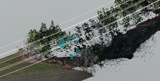
Then, for quantitative analysis, occlusion points were submitted to a voxelization procedure and, lastly, clustered into separate objects (
Figure 19). For each object summary, the approximated volume was calculated as a sum of the volume of all voxels that formed it. Then, all the data were summed up and compared to UAV and TLS data results (
Table 8).
Big differences can be observed between TLS and UAV data. This was to be expected. TLS and UAV products due to their acquisition procedures being widely different. Photogrammetric products do not penetrate greenery, while TLS does. Thus, TLS data have the advantage of a more continuous representation of lattice objects. This can cause an effect of one object in TLS data being represented by multiple objects in UAV data (
Figure 19e,f). As a consequence, the recorded volume of obstacles determined using TLS data will be far higher than using UAV data.
Similarly, very small vegetation elements could have been picked up by TLS but would not come up within dense point cloud reconstruction (
Figure 19a,b). The importance of such objects is negligible. Nonetheless, that also causes differences in the total volume of occlusions. The date of the data acquisition was also not without consequence. Bare trees are quite difficult to reconstruct in photogrammetric data, so—for better results—data should be acquired during the growing season.
4. Discussion
This paper presents a comprehensive method of processing UAV images to detect and reconstruct 3D power lines, then subsequently compare them with a point cloud representation of DSM to localize any objects threatening the safety of the power lines.
Power line inspections are a topical issue these days. Modeling wires in 3D space is essential for the assessment of power line safety. Thus, their reconstruction has received much attention. However, unlike other studies on the subject, this paper presents the entire workflow for corridor clearance monitoring. Each step of the proposed method, starting with data acquisition requirements and ending with obstacle detection, is described comprehensively. The wire detection in UAV images was performed using a decorrelation stretch for initial image processing, the modified Prewitt filter for edge enhancement, and RANSAC with additional parameters for line fitting. This classic approach causes the line extraction in the UAV images to take place in a controlled way and, if necessary, the user can modify the processing parameters (thresholds) and even manually restart the process when detection errors occur. The combination of these elements creates a solution that is robust to low-quality input data (images). Despite a variety of backgrounds and the dubious visibility of wires, the created solution managed to consistently detect power lines in a series of images. Its highest achieved success rate exceeded 98% and remained above 90% for more challenging data. Good performance in the highly changeable environment can be attributed to complete disregard for the wire color, as well as the implementation of a local, ordered approach, which made the method adaptable to both contrast change as well as angle change in the wire positions.
The algorithm does not require an extensive learning set, which makes it different from many deep learning methods [
37,
38], which are currently gaining popularity. Similar to some other solutions [
23,
35,
40,
41], wire reconstruction in 3D space is performed using epipolar geometry. However, the proposed RANSAC-based approach to fit the catenary curve to previously obtained points representing the wires minimizes the noise.
Despite the fact that the algorithm is not completely autonomous, it is relatively flexible and robust. The minor user intervention allows the system to be applied in a variety of cases, either to a low or high voltage. However, there is room for improvement in the proposed method. Such errors as pixel discrepancies due to detection transfer are removed while fitting the chain curve to the 3D data. Others, such as a complete loss of detection, or overlay with neighboring wires, can be solved by implementing a two-step approach: after initial processing, the algorithm automatically directs the user to problematic sections where the process can be restarted or corrected manually.
There are multiple thresholds set in the method, though it must be said that, after an initial threshold sensitivity analysis, none were changed for any of the tested sets, nor in further commercial exploitation.
Another drawback might be the mandatory initial user input. However, it must be stated that this is limited to two points per wire for the whole survey section, which takes no more than a couple of minutes. Many methods can be applied instead of initial user input. The approximate direction based on the positions of the utility poles and the Hough transform [
50] was used to detect the wires in a test phase in this research. The initial results were encouraging for medium-voltage power lines. However, with the diversification of the background and the introduction of wires at multiple heights in high-voltage lines, this method failed. The problem of the relative positioning of wires between images in stereopairs is complex. It is the process of recognizing the same wire in images within a stereopair. As wires are made of the same material, and due to the large distance between the background and them, there is no information linking two images that capture the same wire. An alternative here would be to include a third verification strip of images or to create multiple 3D reconstructions containing all combinations of wires and then deciding on the pairing. The first process would extend the duration of the survey and necessitate different mission planning methodologies. The second would also require either manual input or prior knowledge of the number of wires and types of utility poles.
In many studies on power line inspections, datasets have been small or numerical quality analyses have been omitted [
23,
40,
41]. The method presented in this paper has been profusely tested beyond its scope since it has already been commercially implemented. This study demonstrates that the accuracy of the proposed method for the 3D reconstruction of power lines is consistent with that achieved using classical measurements. Similar accuracies are reported by Oh and Lee [
40], but their accuracy analyses were limited to only two wires whose geometry was determined using the reference method.
It should be noted that none of the verification methods used for accuracy assessment in this study were free from errors or significantly more accurate than any other. As the true value of the measured sag of the wires or their 3D geometry was unknown, it was only possible to assess the mutual compatibility of the methods used, and not their absolute accuracy.
The results of the accuracy assessment described in this paper were also influenced by the fact that surveys of power lines using three methods (UAV, TLS, TS) were not carried out simultaneously, or under the same weather conditions. This was due to the technical feasibility of surveys. For most spans, the TS and TLS measurements were performed in parallel (except for one span of a high-voltage power line) and lasted four days. On the contrary, UAV flights over power lines in Datasets III and IV were completed in one day. For this reason, different conditions of the power lines were recorded between the methods.
The mapping of vegetation around power lines is also an issue of great importance. In this paper, we assessed whether UAV-derived point cloud representations of DSM, generated using a classic approach, are sufficient to monitor power line corridors. In the case of the UAV-based photogrammetric products, the most common error was missing data in representing the DSM. The solution to this was to take UAV images in more than two strips. However, this did not significantly increase the correctness of tree reconstruction for the DSM, which, in turn, was the main reason for incorrect DSM extraction. One way to solve this problem is to capture UAV-based photogrammetric data during the vegetation period. However, as a rule, in the immediate vicinity of the power line (up to ~10 m from the line axis), the quality of the UAV-derived DSM was adequate to analyze the separation between the wires from and elements of the land cover.
5. Conclusions
The aim of this research was to create a novel method based on UAV imagery for occlusion monitoring in the corridor of power lines. The proposed method mainly consists of three parts: the reconstruction of the geometry of the wires in 3D space, the reconstruction of point cloud representation of the DSM, and subsequently detecting obstacles in the power lines corridor. Power line reconstruction, which was carried out using images captured for the DSM calculation, is its essential part. Well-known computer vision algorithms and epipolar geometry were adopted for this task. This makes the proposed method user-friendly and allows for image processing to be performed in a fully controlled way. There are other merits: no training data are required, the method is robust to low-quality input data, and the RANSAC-based approach to model the wires reduces the influence of the noise.
An integral part of the proposed method is a workflow for the detection of obstacles in the power line corridor. Obstacles are selected by calculating the distance between power lines and each point in the point cloud representation of the DSM and simplified into voxels and then objects. The analyzed data are georeferenced. Thus, the parts of the power line corridor where the maintenance work has to be performed are documented using both the precise information of their locations and images.
The feasibility of the proposed UAV-based method for the 3D reconstruction of power lines and corridor clearance monitoring was confirmed by reference surveys. They achieved results similar to those obtained using other available solutions. The method’s relatively high accuracy, comparable with that obtained by means of the reference measurements, was also verified. The accuracy of its 3D reconstruction for medium-voltage power lines was 15 cm. In the case of high-voltage power lines, it did not exceed 30 cm. The proposed method allows for measurement data to be collected in a relatively short time, and is cheaper than other commonly used methods in the area.
In the case of corridor clearance monitoring, the results are also satisfying. Visual analysis proved that obstacles were detected in the same places for both UAV and TLS data. However, there were big differences in the volume of calculated obstacles in between methods. This was expected due to the properties of both data acquisition methods. However, this does not disprove the usability of the method. Crucial obstacles were identified, and the presence of obstacles is of the utmost importance. In future works, more focus should be placed on DSM.
The results of this study were implemented for commercial use by FlyTech UAV. The algorithm has already been used to measure several hundreds of kilometers of power lines.

 ,
, 


