Article

Use of an Active Canopy Sensor Mounted on an Unmanned Aerial Vehicle to Monitor the Growth and Nitrogen Status of Winter Wheat

1
National Engineering and Technology Center for Information Agriculture, Key Laboratory for Crop System Analysis and Decision Making, Ministry of Agriculture, Jiangsu Key Laboratory for Information Agriculture, Jiangsu Collaborative Innovation Center for Modern Crop Production, Nanjing Agricultural University, 1 Weigang Road, Nanjing 210095, China
2
Department of Agronomy and Horticulture, University of Nebraska-Lincoln, Lincoln, NE 68583, USA
*
Author to whom correspondence should be addressed.
The first two authors contributed equally to this work.
Remote Sens. 2020, 12(22), 3684; https://doi.org/10.3390/rs12223684
Submission received: 19 September 2020 / Revised: 21 October 2020 / Accepted: 31 October 2020 / Published: 10 November 2020
(This article belongs to the Special Issue Remote and Proximal Sensing for Precision Agriculture and Viticulture)

Abstract

:
Using remote sensing to rapidly acquire large-area crop growth information (e.g., shoot biomass, nitrogen status) is an urgent demand for modern crop production; unmanned aerial vehicle (UAV) acts as an effective monitoring platform. In order to improve the practicability and efficiency of UAV based monitoring technique, four field experiments involving different nitrogen (N) rates (0–360 kg N ha−1) and seven winter wheat (Triticum aestivum L.) varieties were conducted at different eco-sites (Sihong, Rugao, and Xinghua) during 2015–2019. A multispectral active canopy sensor (RapidSCAN CS-45; Holland Scientific Inc., Lincoln, NE, USA) mounted on a multirotor UAV platform was used to collect the canopy spectral reflectance data of winter wheat at key growth stages, three growth parameters (leaf area index (LAI), leaf dry matter (LDM), plant dry matter (PDM)) and three N indicators (leaf N accumulation (LNA), plant N accumulation (PNA) and N nutrition index (NNI)) were measured synchronously. The quantitative linear relationships between spectral data and six growth indices were systematically analyzed. For monitoring growth and N nutrition status at Feekes stages 6.0–10.0, 10.3–11.1 or entire growth stages, red edge ratio vegetation index (RERVI), red edge chlorophyll index (CIRE) and difference vegetation index (DVI) performed the best among the red edge band-based and red-based vegetation indices, respectively. Across all growth stages, DVI was highly correlated with LAI (R2 = 0.78), LDM (R2 = 0.61), PDM (R2 = 0.63), LNA (R2 = 0.65) and PNA (R2 = 0.73), whereas the relationships between RERVI (R2 = 0.62), CIRE (R2 = 0.62) and NNI had high coefficients of determination. The developed models performed better in monitoring growth indices and N status at Feekes stages 10.3–11.1 than Feekes stages 6.0–10.0. To sum it up, the UAV-mounted active sensor system is able to rapidly monitor the growth and N nutrition status of winter wheat and can be deployed for UAV-based remote-sensing of crops.

Graphical Abstract

1. Introduction

Overapplication of nitrogen (N) fertilizers is a common problem in crop production. Precision N management is developed to improve N use efficiency by matching fertilizer N input with spatial and temporal crop N demand [1,2]. Crop growth and N nutrition status estimation is prerequisite for determining optimal N application rate; remote sensing techniques act as a rapid, nondestructive and efficient method.
Remote sensing has been widely applied for monitoring crop growth and N nutrition indicators, the main platforms include satellite [3,4], aerial [5,6] and ground platforms [7,8]. Satellites can monitor large crop areas for precision management, and satellite data have been effectively used to monitor aboveground dry matter and N accumulation in winter wheat [9,10]. However, the quality of remote sensing data from passive sensor-based satellites should be easily affected by cloudy or rainy weather conditions, which leads to the lack of applicable real-time sensing datasets for crop monitoring [11,12]. Ground sensing platforms are easy to operate and produce highly repeatable data for monitoring crop growth. For example, data from ground-based hyperspectral sensing have high resolution and continuity, and this sensing platform has been used to estimate plant and leaf N content in winter wheat [13,14]. However, hyperspectral sensors use a wide range of wavebands, producing massive datasets that require time-consuming data processing [15]. Additionally, hyperspectral sensors mainly use passive light sources and have strict requirements for proper function with respect to light intensity and other environmental conditions. Thus, the use of these sensors is restricted by weather and other environmental factors [16]. Active sensors are equipped with an internal light source, which can mitigate the influence of cloud cover and other suboptimal environmental conditions. Portable active canopy sensors, such as GreenSeeker and Crop Circle, have been used widely in precision crop management [17,18]. GreenSeeker sensors have been used to estimate wheat N status and rice yield [19,20]. However, default values of the normalized difference vegetation index (NDVI) exported from the sensor were saturated when crop populations were large; thus, unreliable data were produced during the late growth period [21]. The Crop Circle ACS-470 sensor has six wavebands: 450, 550, 650, 670, 730 and 760 nm. Several potential spectral vegetation indices can be constructed by combining different bands, and such indices have been used successfully to estimate wheat and corn N status [22,23]. Holland Scientific has developed another active canopy sensor, RapidSCAN CS-45, which has three fixed wavebands covering red (670 nm), red edge (730 nm) and near-infrared (780 nm) regions. Therefore, many potential vegetation indices could be derived by the spectral data collected using this sensor. For example, the red band can be used to calculate different red-based vegetation indices, such as common difference vegetation index (DVI) and NDVI, which have been used for successfully monitoring rice LAI [24], maize N status [18] and wheat yield [25]. Otherwise, the red edge-based vegetation indices also have been proved a consistent good performance for crop growth estimation. Erdle et al. [26] compared three different active and passive spectral sensors to discriminate biomass parameters and nitrogen status in wheat and found the red edge ratio vegetation index (RERVI, R760/R730) was the most powerful and temporally stable spectral index for monitoring wheat biomass and N status among all indices tested. Several studies also ascertained strong relationships between the red-edge band and LAI of several crops [27,28]. As a result, it is necessary to evaluate the performance of different vegetation indices derived from the RapidSCAN CS-45 sensor for winter wheat growth and N status estimation.
Active sensors performed well for crop growth and N status estimation, however, it has mainly been developed for close distance analyses (as e.g., on board of tractors) due to measurement height limitation [29], while installation on aerial platforms is less usual. The RapidSCAN CS-45 sensor runs on the novel Pseudo Solar Reflectance (PSR) technology that allows for height-independent measurement. Thus, this type of active sensor can be carried on a low-altitude platform to collect data at a broad spatial scale [30]. Remote sensing using aerial platforms represents a good compromise between ground- and satellite-based platforms. For example, manned aircraft have been used to monitor crop growth [31,32]. However, this method is costly and requires experienced labor, and is thus not practical for frequent use in farm production. Unmanned aerial vehicles (UAVs) are operated at lower costs and require less skilled labor but still produce data with high spatial resolution. Although some factors may affect this vehicle operability, such as payload capacity, flight duration, legal aspects, ground area covered in each flight, etc., UAVs have been widely used to monitor crop leaf area index (LAI; [33]), biomass [34], and N nutrition indicators [35] and to predict crop yield [36]. Most of the sensors mounted on UAVs in previous studies were passive hyperspectral, multispectral or simple digital cameras [37,38,39]. These require complicated and time-consuming image analyses, which are challenging for operators without specialized skills or equipment. To date, little research has been conducted on the suitability of using active sensors on UAVs.
While active sensors mounted on manned aircraft and UAVs have been used to monitor the vigor and N status of maize and sorghum [30,40], the use of UAV-based active sensing to monitor the growth of winter wheat has not been studied. Additional indicators of growth and N nutrition are needed. Therefore, the objectives of this study were to (1) develop a rapid data acquisition method based on a UAV-mounted RapidSCAN CS-45 sensor and (2) construct spectral monitoring models for three growth indicators—LAI, leaf dry matter (LDM) and plant dry matter (PDM) and three N nutrition indicators—leaf N accumulation (LNA), plant N accumulation (PNA) and N nutrition index (NNI) of winter wheat. The results of our study will be useful for improving real-time methods to acquire crop growth and N nutrition status and for guiding appropriate N management.

2. Materials and Methods

2.1. Study Site and Experimental Design

This study was conducted in Jiangsu Province, east China. Experiments 1 (2015–2016) and 3 (2016–2017) were conducted at Sihong Experimental Station (33.37°N, 118.26°E) using two winter wheat varieties, “Xumai30” and “Huaimai20”, grown at five N levels: 0, 90, 180, 270, and 360 kg N ha−1. Plants were spaced 25 cm apart and grown at a density of 2.25 million seedlings ha−1. Experiment 2 was conducted at Rugao Experimental Station (32.27°N, 120.75°E) from 2016 to 2017, using two winter wheat varieties, “Yangmai15” and “Yangmai16”, at three N levels: 0, 150 and 300 kg N ha−1. Plants were spaced 25 cm apart and grown at density of 3.00 million seedlings ha−1 and 1.50 million seedlings ha−1. Experiment 4 (2018–2019) was conducted at Xinghua Experimental Station (33.08°N, 119.98°E) using three winter wheat varieties, “Zhenmai12”, “Yangmai23”, and “Ningmai13”, grown at five N levels: 0, 90, 180, 270 and 360 kg N ha−1. Plants were spaced 25 cm apart and grown at a density of 2.25 million seedlings in each hectare. Above seven varieties are the main planting cultivars in Jiangsu Province, which all belong to semiwinter wheat cultivars. The major differences between cultivars are plant type and height.
We used a randomized complete block design with three replicates for each treatment. Plot size was 42 m2 (6 m × 7 m) in Experiments 1 and 3, 30 m2 (5 m × 6 m) in Experiment 2 and 63 m2 (7 m × 9 m) in Experiment 4. The varieties were sown separately by manual seeding in each plot. Granular urea was used as N fertilizer in all experiments and applied in two batches: 50% before sowing and 50% at the wheat jointing stage (Feekes stages 6.0). Based on the results of soil analysis and the recommendations from the local agricultural department, 105 kg P2O5 ha−1 was applied before sowing in the form of Ca (H2PO4)2 and 135 kg K2O ha−1 was applied as two splits: 50% before sowing and 50% at the stem elongation stage. Irrigation was applied one time to ensure the seeds germinated securely after sowing if there was no rainfall. Sihong experimental station is located in warm temperate monsoon climate zone, which receives approximately 2300 h of sunshine and 910 mm rainfall annually, with average temperature of 16.2 °C. Rugao experimental station is in north subtropical humid climate zone, which receive approximately 2100 h of sunshine and 1050 mm rainfall annually, with average temperature of 16.7 °C. Xinghua experimental station sites are in subtropical monsoon climate zone, which receive approximately 2120 h of sunshine and 900 mm rainfall annually, with average temperature of 17.3 °C. Detailed information can be found in Table 1.

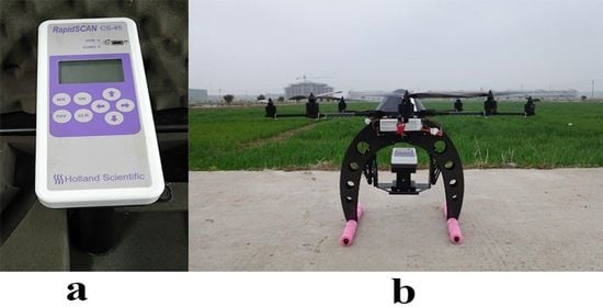
2.2. Spectral Data Collection

The RapidSCAN CS-45 sensor (Figure 1a; www.hollandscientific.com) weighs 0.8 kg and has three fixed wavebands: red (R; 670 ± 5.5 nm), red edge (RE; 730 ± 5.5 nm) and near-infrared (NIR; 780 ± 10 nm). The two default vegetation indices produced by the sensor are the normalized difference red edge (NDRE) and NDVI. Sensor memory module automatically records the spectral reflectance (%) of the wheat canopy in each band, the default vegetation indices and Global Positioning System (GPS) data at a frequency of 2.5 Hz (one reading per 0.4 s). The data is exported as a .csv file by PC software. The spectral bands of sensor are scaled as percentages and will not vary with sensor height above a planar target; this technology named PSR measurement ensures a degree of data stability within an effective sensing distance (0.3–3 m above the canopy as introduced by the manufacturer). Therefore, RapidSCAN CS-45 is feasible to mount on the UAV (Figure 1b; Mikrokopter OktoXL DW03; Beijing Esky Tec. Ltd., Beijing, China) for practical application [30]. Before the flight, the UAV’s own platform maintained a fixed posture after passing the self-test, the sensor was mounted on the UAV’s platform using a customized gimbal and then the sensor’s light source was pointed downward vertically via adjusting UAV’s platform angle. The sensor was manually triggered on to start collecting data, then triggered off after the flight of the UAV. The UAV was flown automatically along predetermined flight routes that aligned with the central axis of each plot, at a height of 1.5 m above the canopy and a heading speed of 2 m s−1. The resulting field of view had an area of 0.33 m2.
The spectral data were processed in ArcMap 10.5 (ESRI, Redlands, CA, USA) and assigned to different sampling plots with the GPS position of each reading point. The yellow dots in Figure 2 indicate the test points recorded by the UAV-mounted RapidSCAN CS-45 sensor. The UAV flew two times over each plot, the second flight was inverted with respect to the first one (Figure 2) and a buffer of approximate 0.5 m was used to exclude the data near the plot boundary, then the reflectance values of two measurements collected by the sensor were averaged to represent the spectral data of each plot. Monitoring was conducted at the jointing (Feekes growth stages 6.0–9.0), booting (Feekes growth stage 10.0), heading (Feekes growth stage 10.3), flowering (Feekes growth stage 10.5.2) and filling stages (Feekes growth stage 11.1) [41]. Data obtained by the sensor included spectral reflectance values in the R, RE and NIR bands, which were used to calculate vegetation indices, as detailed in Table 2.

2.3. Plant Sampling and Measurements

For field experiments where each plot is often small (42 m2 in Experiments 1 and 3, 30 m2 in Experiment 2 and 63 m2 in Experiment 4) and grown homogeneously, it is common to take representative destructive samples and canopy spectral measurements at different positions within each plot [7,17]. Once spectral data were collected, the plants in the corresponding plots were destructively sampled synchronously. Twenty plants in the corresponding plots were randomly sampled and averaged in each plot. The plants were separated into stems and leaves. The LAI was measured using a Li-3000c leaf area meter (Li-Cor, Lincoln, NE, USA). Each subsample of stem and leaf was oven-dried for 30 min at 105 °C to stop all plant metabolic activities, and then dried at 80 °C until it reached a constant weight. The weight of each subsample was recorded at this point, and LDM and PDM were determined. The N nutrition indicators, such as leaf N content (LNC) and stem N content (SNC), were measured using the micro-Kjeldahl method [54].
LNA and PNA were then calculated as follows:
LNA ( kg · ha 1 ) = LDM ( kg · ha 1 ) × LNC ( % )
PNA ( kg · ha 1 ) = LDM ( kg · ha 1 ) × LNC ( % ) + SDM ( kg · ha 1 ) × SNC ( % )
where LDM and SDM (kg ha−1) are the dry matters weight of leaves and stems, LNC and SNC are the N concentrations of the leaves and stems, respectively.
We used the critical N dilution curve of winter wheat developed by Zhao et al. [55] in this study:
N cnc = 4.33 DM 0.45
where Ncnc is the critical N concentration [56] and DM is the aboveground biomass equivalent to PDM (t ha−1).
The NNI was calculated according to the equation developed by Gilles et al. [57]:
NNI = N a N cnc
where Na is the actual measured N concentration and Ncnc is the critical N concentration as determined by Equation (3).

2.4. Statistical Analyses

Data collected from Experiments 1, 2 and 3 were used to determine the linear relationships between the vegetation indices and the growth and N nutrition indicators; the data from Experiment 4 was used to validate the accuracy of developed models. The coefficients of determination (R2) of the relationships between the vegetation indices and growth indicators, and between the vegetation indices and N nutrition parameters, were calculated using Microsoft Excel (Microsoft Corporation, Redmond, WA, USA). The models with the highest R2 were then selected. The scatter diagrams of the selected vegetation indices-based models were plotted using GraphPad Prism 6 (GraphPad Software Inc., San Diego, CA, USA). Additionally, model performance in predicting winter wheat growth and N nutrition indicators was evaluated using root mean square error (RMSE) and bias, which were calculated as:
RMSE = 1 n × 1 n ( P i Q i ) 2
Bias = 1 n ( P i Q i ) / n
where n is the number of samples, Qi is the observed value and Pi is the value derived from the model.

3. Results

3.1. Variability of Wheat Growth and Nitrogen Status Indicators

The growth (LAI, LDM, PDM) and N (LNA, PNA, NNI) indicators varied greatly across all growth stages, different N treatments, varieties and site-years (Table 3). For calibration data, the PNA was most variable (coefficient of variation (CV) = 71.70%) across all growth stages, followed by LNA (CV = 70.11%), LAI (CV = 60.08%), PDM (CV = 57.14%) and LDM (CV = 51.00%), and NNI had the lowest coefficient of variation (43.28%). The analysis showed that LDM, PDM, LNA and PNA were more variable during Feekes stages 6.0–10.0 (CV = 53.46%, 56.31%, 72.79% and 70.04%, respectively) than Feekes stages 10.3–11.1 (CV = 49.49%, 35.46%, 66.61% and 62.09%, respectively), and LAI, NNI showed more variable during Feekes stages 10.3–11.1 (CV = 62.21% and 44.44%, respectively) than stages 6.0–10.0 (CV = 52.24% and 40.63%, respectively). This was similar for both the calibration and validation experiment datasets. The large variability of these parameters made it possible to evaluate the performance of using the sensor for estimating winter wheat growth and N status.

3.2. Dynamic Changes in Vegetation Indices

The dynamic temporal changes in the default vegetation indices with Feekes growth stages of Huaimai20 in Experiment 1 are displayed in Figure 3. The vegetation indices exhibited similar trends in all N treatments as wheat growth progressed. NDRE values increased slowly and then gradually decreased (Figure 3a). In contrast, NDVI values increased slowly and then remained high (Figure 3b). The values of the vegetation indices of plants treated with high N levels were generally higher than those of plants treated with low N levels, indicating that increased amounts of N fertilizer led to changes in leaf color, which then resulted in higher vegetation index values. The NDRE represented the growth process of winter wheat better than the NDVI. Figure 3b showed a crossing of the NDVI course between N2 (180 kgN/ha) and N3 (270 kgN/ha) treatment; the NDVI values under N3 treatment are lower than that under N2 treatment before Feekes growth stage 10.0. This phenomenon may be due to the N2 and N3 plots having similar growth status after N topdressing (NDRE course also showed the close values between N2 and N3 treatments), but the NDVI index cannot well distinguish this difference.

3.3. Relationships between Crop Growth Indicators and Vegetation Indices

Growth indicators such as LAI, LDM and PDM were obtained for each spectral sensing period. We considered two general wheat growth stages: before heading (Feekes stages 6.0–10.0) and after heading (Feekes stages 10.3–11.1); all growth stages were also considered separately. Based on the vegetation indices listed in Table 2, quantitative relationships between vegetation indices and growth indicators were systematically analyzed. Table 4 lists the top 6 vegetation indices (listed with descending order based on R2 values) based on spectral reflectance values exported from the RapidSCAN CS-45 sensor, which were used to establish linear regression models with growth indicators of winter wheat. Vegetation indices were better at monitoring the LAI, LDM and PDM of winter wheat at Feekes stages 10.3–11.1 than at Feekes stages 6.0–10.0. At Feekes stages 6.0–10.0 and 10.3–11.1, and across all growth stages, the relationships between vegetation indices and LAI had R2 values of 0.73–0.88, and the RERVI and red edge chlorophyll index (CIRE) had higher correlation with LAI than other vegetation indices, with R2 values of more than 0.75 at Feekes stages 6.0–10.0 and 10.3–11.1, and across all growth stages. At Feekes stages 6.0–10.0, R2 values for the relationships between vegetation indices and PDM ranged from 0.62 to 0.64, which were slightly higher than the R2 values for relationships with LDM (R2 = 0.59–0.61). The DVI was most closely associated with LDM (R2 = 0.61) and PDM (R2 = 0.64) at Feekes stages 6.0–10.0. At Feekes stages 10.3–11.1, R2 values for associations between vegetation indices and LDM ranged from 0.70 to 0.78, which were slightly higher than the R2 values for associations with PDM (R2 = 0.68–0.73). The DVI was the top vegetation indice for estimating LDM (R2 = 0.78) and PDM (R2 = 0.73) at Feekes stages 10.3–11.1. Across all growth stages, the values of R2 for vegetation indices-LDM relations ranged from 0.59 to 0.61, and the DVI, RERVI and CIRE were most closely associated with LDM (R2 = 0.61). The values of R2 for vegetation indices-PDM relations ranged from 0.54 to 0.63, and the DVI and RVI were most closely associated with PDM (R2 = 0.60–0.63) across all growth stages.

3.4. Relationships between N Nutrition Indicators and Vegetation Indices

We used linear regression to analyze the relationships between vegetation indices calculated from the spectral reflectance data collected by the RapidSCAN CS-45 sensor and N nutrition indicators, namely, LNA, PNA and NNI. We selected top 6 vegetation indices (listed with descending order based on R2 values) to establish linear regression models with N nutrition indicators of winter wheat at Feekes stages 6.0–10.0 and 10.3–11.1, and across all growth stages (Table 5). At Feekes stages 6.0–10.0, R2 values for associations with LNA, PNA and NNI ranged from 0.61 to 0.66, 0.60 to 0.65 and 0.48 to 0.52, respectively. The DVI, RERVI and CIRE were more closely associated with N nutrition indicators (R2 = 0.50–0.66) at Feekes stages 6.0–10.0. At Feekes stages 10.3–11.1, the relationships between vegetation indices and LNA, PNA and NNI had R2 values of 0.65–0.72, 0.75–0.82 and 0.75–0.81, respectively, and the best performing vegetation index for estimating N nutrition indicators was DVI (R2 = 0.72–0.82). Across all growth stages, R2 values for associations with LNA, PNA and NNI ranged from 0.61 to 0.65, 0.65 to 0.73 and 0.58 to 0.63, respectively. The DVI, RERVI and CIRE were more closely associated with N nutrition indicators (R2 = 0.62–0.73) across entire growth stages.

3.5. Model Validation

Data collected from Experiment 4 was used to validate the top 6 regression models developed in this work, and verification results were listed with ascending order based on RMSE values (Table 6 and Table 7). At Feekes stages 6.0–10.0, 10.3–11.1 and across entire growth stages, the predictions of growth (LAI, LDM and PDM) and N (LNA, PNA and NNI) indicators mostly underestimate the actual values with the bias values less than 0 (Table 6 and Table 7). At Feekes stages 6.0–10.0, the results indicated that DVI performed better than other vegetation indices for estimating agronomic indicators (Figure 4a–e, R2 = 0.56–0.74), except PDM, which was more strongly related with RERVI (Figure 4f, R2 = 0.61) and CIRE (R2 = 0.61). At Feekes stages 10.3–11.1, the validation results showed that DVI performed better than other vegetation indices for estimating LAI (Figure 5a, R2 = 0.69), LDM (Figure 5b, R2 = 0.69), PDM (Figure 5c, R2 = 0.43) and PNA (Figure 5d, R2 = 0.68), while RERVI performed well for estimating LNA (Figure 5e, R2 = 0.75) and NNI (Figure 5f, R2 = 0.78). Across all growth stages, the validation results indicated that DVI performed better than other vegetation indices for estimating growth and N indicators (Figure 6a–e, R2 = 0.32–0.72), except NNI, which was more closely associate with RERVI (Figure 6f, R2 = 0.41) and CIRE (R2 = 0.41). Overall, at Feekes stages 6.0–10.0, 10.3–11.1 and across entire growth stages, the RERVI, CIRE and DVI were better for predicting growth and N nutrition status than other RE and R bands-based vegetation indices, respectively.
Based on the results of establishment and validation of the models, several vegetation indices performed consistently well in agronomic indicators estimation during each growth stage. At Feekes stages 6.0–10.0, DVI was the best index at predicting LDM, LNA, PNA and NNI. Conversely, RERVI and CIRE based monitoring models predicted LAI and PDM most accurately among these vegetation indices used in this study. At Feekes stages 10.3–11.1, the best performing vegetation index for estimating growth and N nutrition status was DVI. Across all growth stages, DVI models were the best at predicting growth and N nutrition indicators, except RERVI and CIRE performed best for estimating NNI among these vegetation indices discussed in this study.

4. Discussion

In this study, we analyzed dynamic changes in the NDRE (Figure 3a) and NDVI (Figure 3b) as calculated from data obtained by a UAV-mounted RapidSCAN CS-45 sensor. The dynamic tendency of NDRE under 180 (N2), 270(N3) and 360 (N4) kg/ha N treatments showed strong similarity, which may be the result of decrease of crop N uptake efficiency under high N application rates. Previous studies also indicated that the limitation of crop N uptake efficiency due to too high availability of N in the soil [58,59]. The NDVI remained high at the late growth stages (Figure 3b) and was likely saturated at high plant biomass [17]. The R band becomes saturated with canopy closure and reduced penetration of visible light and NIR into the canopy, thus affecting vegetation indices which involve R band [60]. Similar results have been reported for monitoring growth status of rice [61], spring maize [18] and winter wheat [26]. In contrast, RE radiation can penetrate deeper into the crop canopy due to its lower absorption by chlorophyll. The dynamic changes of NDRE (Figure 3a) represented the growth process of winter wheat better than the NDVI (Figure 3b), which is consistent with the fact that the RE band is less likely to be saturated compared to the R band [62]. As expected, vegetation indices that use the RE band such as RERVI was better at predicting growth and nutrition indicators in our study. For example, at Feekes stages 6.0–10.0, 10.3–11.1 and across entire growth stages, RERVI (R2 = 0.50–0.88) was highly correlated with growth (LAI, LDM, PDM) and N nutrition (LNA, PNA, NNI) indicators. Similarly, vegetation indices that use RE bands were reported to be better at predicting LAI [28,63], chlorophyll content [64], and N concentration [65], and were less affected by saturation effects in contrast to indices that use R bands. Additionally, the NIR band is reported to be closely associated with crop canopy architecture and plant intracellular airspaces and allows for deep canopy exploration even with high aboveground biomass [66,67], consistent with our results.
As in previous studies that considered a suite of agronomic parameters [17,61,68], we tested a UAV-mounted RapidSCAN CS-45 active canopy sensor to monitor six growth and N nutrition indicators (LAI, LDM, PDM, LNA, PNA and NNI) in this study. Among the determination of the models, the DVI was highly correlated (R2 = 0.52–0.87) with growth and N nutrition indicators at Feekes stages 6.0–10.0 and 10.3–11.1, and across all growth stages. The DVI (R2 = 0.57) had a similar, slightly higher correlation with vine LAI than the NDVI (R2 = 0.53) or RVI (R2 = 0.54) in a study using satellite data [69] and predicted rice LAI (R2 = 0.80) most accurately at the panicle-initiation stage in a study using a UAV-based remote sensing system [24]. The DVI can also be used to accurately estimate crop characteristics and classification [70,71] and to predict winter wheat yield [25] (The yield information in this study is shown in Supplementary file—Table S1 and Figure S1). In this study, the LAI estimation (Table 4: R2 = 0.73–0.88) performed relatively better than that of LDM (Table 4: R2 = 0.59–0.78) and PDM (Table 4: R2 = 0.54–0.73) at Feekes stages 6.0–10.0 and 10.3–11.1, and across all growth stages; this might be because the LAI is significant canopy-structure-parameter, which largely dominate the canopy reflectance [72]. Previous studies also indicated that the LAI was better performing compared to biomass estimation [73,74], which were consistent with our study. During the validation of the models (Figure 4, Figure 5 and Figure 6), the predictions of agronomic indicators mostly underestimate the actual values, for example, the LDM model (Figure 4b) had a slope of 1.00, but the intercept of 0.13 and the bias of −0.13 caused the model to underpredict LDM at Feekes stages 6.0–10.0; at Feekes stages 10.3–11.1, the PNA model (Figure 5d; slope = 0.77, intercept = 27.87, bias = −8.45 kg ha−1) appeared to underestimate actual values particularly for lower PNA (<121 kg ha−1); the LAI model (Figure 6a) showed overall underestimation with a bias of -0.42 across all growth stages, further, the intercept (0.85) and slope (0.84) of the model indicated that the model underpredicts LAI for values ≤ 5.3 and overpredicts LAI for values > 5.3. The difference of plant type and height affected the spectral reflectance among different wheat varieties [75], which may lead to the difference between predicted and observed values. Previous studies also indicated that the spectral difference of crop cultivars results in the estimated deviation of agronomic parameters [76,77]. Thus, more abundant data from different years, ecological sites and varieties should be considered to construct the more universal estimation model in future study.
Modeling scores were higher at Feekes stages 10.3–11.1 than 6.0–10.0 in this study, probably because the vegetation was sparse (no canopy closure) at early growth stage and spectral reflectance was more influenced by the bare soil surface; previous studies also found this similar phenomenon in predicting leaf nitrogen content and plant N uptake of winter wheat and rice NNI during early growth stages [23,78]. Soil adjusted vegetation index (SAVI) was used to eliminate the influence of soil [45], but it exhibited low efficiency in this study. Other studies found that fluorescence sensing could detect N variability as early as at the V5 stage (Feekes stages 5.0 in wheat) of maize and was not influenced by soil background [79]. Across all growth stages, the validation results of estimation models, such as PDM (Figure 6c) and NNI (Figure 6f), showed the separation of scatter points between before and after heading stages, the emergence of spike may influence the performance of spectral models at the late growth stages [80,81], other studies also indicated the influence of growth stages on agronomic parameters estimation [82,83]. Several growth stages were considered in two general categories: before and after heading stages in this study. Thus, the developed models are more flexible and allow for indicators to be monitored at each growth stage.
UAV-based sensors mainly comprise multispectral, hyperspectral and simple RGB cameras, which can provide image-based data for several spectral indices to estimate crop growth and N status [37,38,39]. However, the processing of these image-based data, which includes image capturing and splicing, geometric correction and extraction of useful spectral data, is complex and often time-consuming, especially when data are collected over large areas. Data processing also requires high-performance computers, specific software and highly trained technical staff [5]. UAV-based remote sensing system used passive optical sensors, which are susceptible to the light intensity and monitoring conditions [23]. In contrast, the active canopy sensor used in this study is not influenced by ambient illumination, as it has an internal polychromatic light source. Therefore, data acquisition using this active sensor is not affected by sampling time or weather, and the data on crop growth have been used to identify the N nutrition status of crops [84], to monitor rice N status and soybean productivity [85,86] and to select wheat cultivars in real time [87]. Additionally, geotagged spectral data can be exported directly as a .csv file from the sensor without preprocessing, and the vegetation indices could be directly calculated according to three band (R, RE, NIR) reflectance values. In general, the sensor is suitable for monitoring crop growth status by common user at critical diagnosis period. According to the manufacturer’s instructions, the spectral reflectance bands of RapidSCAN CS-45 sensor are scaled as percentages and will not vary with sensor height above a planar target, which ensures the sensor can be carried on a low-altitude platform to collect data at a large scale. The UAV-mounted RapidSCAN CS-45 sensor has been used to monitor maize N status by manually operating the UAV at heights of 0.5 to 1.5 m [30]. The UAV used in this study was flown automatically along predetermined flight routes that aligned with the central axis of each plot at a height of 1.5 m above the wheat canopy, and at a speed of 2 m s−1. Previous studies showed that 40 h were needed to collect 20,000 plots’ (1 m wide by 4 m long) spectral data on single rows using a single vehicle at speed about 0.56 m s−1, and it would be more time-consuming by handheld sensing (about 0.5 m s−1; [29]). The UAV sensing system in this study had approximate flight duration of 20 min and could run close to 2400 m per set battery charge. Therefore, the data acquisition method based on a UAV-mounted RapidSCAN CS-45 sensor is practicable for monitoring crop growth status at moderate and large scale application. Yet some points still need to be addressed for the practical application of this data acquisition method. (1) As shown in Figure 2, the spectral data points of RapidSCAN CS-45 should be assigned to different sampling plots for data extraction, so a geotagged orthographic image of the measurement area is needed before the data collection. (2) Both the UAV’s automatic flight and the data collection of sensor depend on its own GPS information, therefore, more accurate geographic location information would help in data acquisition. In the current market of UAV applications, Real-Time Kinematic GPS (RTK GPS) could provide centimeter-level high accuracy 3D positioning of the drone [88], this powerful technology would facilitate better application of the UAV-sensing system. (3) As introduced in the Materials and Methods section, the sensor was manually triggered on to start collecting data, then triggered off after the flight of the UAV. If the sensor could be activated automatically at the start point of measurement area, and turned off automatically at the end point, then the data acquisition will be more convenient. This should be considered in future study. (4) Although the sensing data processing of this UAV sensing system was relatively simple, it is necessary to develop automatic procedures for real time data transmission and processing, which would help to further crop management. (5) Payload weight limitations for UAV are generally 20–30% of the total weight of the system [89], the RapidSCAN CS-45 sensor weighs 0.8 kg, which needs to be mounted on the relatively large UAV platform. (6) The short flight duration was a significant restriction for development of traditional multirotor UAV, and the flight duration was approximately 25 min for the majority of the current multirotor UAV system [90]. For a larger area application, the battery and other power performance of UAV still should be improved to increase the flight duration. (7) The cost of UAV used in this study range up to US$ 28,000 and for that of the RapidSCAN CS-45 sensor upwards of US$ 5000. However, it is anticipated that a gradual drop in UAV prices may occur in the near future given increasing competition between UAV producers and the increasing civilian applications of UAV.
In this study, the estimation models of PDM (R2 = 0.63), PNA (R2 = 0.65) and NNI (R2 = 0.52) in winter wheat were established at Feekes stages 6.0–10.0, which covered the critical topdressing N periods (Feekes stages 6.0) for wheat production in study area [7]. The N accumulation during this period could effectively contribute to spikelet production and grain filling in cereals. So, it is advisable to confirm sufficient N accumulation prior to the onset of reproductive phase for grain filling. Previous studies used PNA difference calculated by the estimated PNA minus the critical PNA to guide in-season topdressing N application. For example, researchers took the regional optimal N rates (100 kg N ha−1) as the rice initial total N rate, with 40% and 30% being applied as basal and tillering N fertilizers, respectively, in the Sanjiang Plain of Northeast China. For topdressing N application at the rice stem elongation stage, 30% of the initial total N rate were applied if the N status was optimal. Otherwise, the topdressing N rates can be adjusted based on deficient or surplus N amounts (PNA difference; [78]). Giletto and Echeverría [91] also calculated the potato N requirement (the gap between plant N uptake and critical N uptake) to correct N deficiency, but this method is time consuming and complex. Meanwhile, a favorable relationship (R2 = 0.98) between N requirements and NNI were observed. Yao et al. [59] also indicated a good relationship between wheat N deficit and NNI in Feekes growth stages 5.0 (R2 = 0.82), 6.0 (R2 = 0.82), 10.0 (R2 = 0.91) and 10.3 (R2 = 0.89), which means the real time estimation of NNI had potential to guide in season topdressing N application. The UAV mounted active canopy sensor could be used to nondestructively determine crop N status, and further studies are required to assess whether the UAV sensing system in this study can be applied for in-season topdressing N.
Due to time and labor required to obtain synchronously agronomic parameters, this work mainly analyzed the growth stages start at Feekes stages 6.0. Monitoring frequency before Feekes stages 6.0 could be increased in future studies to improve the model accuracy for each spectral indicator, further improving crop N management. Additionally, similar investigations could be conducted for different crop species in other ecological areas, to further our knowledge of monitoring models and indicators.

5. Conclusions

Our results demonstrated that a UAV-mounted RapidSCAN CS-45 sensor can be used to monitor the growth and N nutrition status of winter wheat. For monitoring growth and N nutrition status at Feekes stages 6.0–10.0, 10.3–11.1 or across all growth stages, the RERVI, CIRE and DVI performed the best among the RE-based and R-based vegetation indices, respectively. Across all growth stages, the DVI was highly correlated with LAI (R2 = 0.78), LDM (R2 = 0.61), PDM (R2 = 0.63), LNA (R2 = 0.65) and PNA (R2 = 0.73). Similarly, RERVI (R2 = 0.62) and CIRE (R2 = 0.62) showed a stronger relationship with NNI than other vegetation indices. The monitoring models predicted each indicator more accurately at Feekes stages 10.3–11.1 than at Feekes stages 6.0–10.0. We conclude that the use of a UAV-mounted active canopy sensor is appropriate for rapid and nondestructive monitoring of the growth and N nutrition indicators of winter wheat. Thus, we recommend this remote-sensing platform and data acquisition method for monitoring crop growth and N status.

Supplementary Materials

The following are available online at https://www.mdpi.com/2072-4292/12/22/3684/s1, Figure S1: The associations between the DVI and yield of winter wheat at Feekes growth stages (a) 6.0, (b) 9.0, (c) 10.3, and (d) 10.5.2 across varieties, sites, and years, Table S1: Coefficients of determination (R2) for pair-wise associations between top 6 vegetation indices and yield of winter wheat at different growth stages across varieties, sites, and years.

Author Contributions

J.J., Z.Z. and X.L. conceived and designed the experiments, J.J., Z.Z. and Y.L. performed experiments with support by Y.T. and Q.C., J.J. and Z.Z. analyzed the data, J.J. and X.L. wrote the paper, B.K., W.C. and Y.Z. provided advice and edited the manuscript. All authors have read and agreed to the published version of the manuscript.

Funding

The work was funded by the Key R&D Program of Jiangsu (BE2019386, BE2018362), the earmarked fund for Jiangsu Agricultural Industry Technology System (JATS[2019]433, JATS[2019]141).

Acknowledgments

We would like to thank Ke Zhang, Songyang Li, and Jiayi Zhang for their help and valuable advice.

Conflicts of Interest

The authors declare no conflict of interest.

References

  1. Zhang, K.; Yuan, Z.; Yang, T.; Lu, Z.; Cao, Q.; Tian, Y.; Zhu, Y.; Cao, W.; Liu, X. Chlorophyll meter–based nitrogen fertilizer optimization algorithm and nitrogen nutrition index for in-season fertilization of paddy rice. Agron. J. 2020, 112, 288–300. [Google Scholar] [CrossRef]
  2. Singh, B.; Singh, V.; Singh, Y.; Thind, H.S.; Kumar, A.; Choudhary, O.P.; Gupta, R.K.; Vashistha, M. Site-Specific Fertilizer Nitrogen Management Using Optical Sensor in Irrigated Wheat in the Northwestern India. Agric. Res. 2017, 96, 159–168. [Google Scholar]
  3. Battude, M.; Al Bitar, A.; Morin, D.; Cros, J.; Huc, M.; Sicre, C.M.; Le Dantec, V.; Demarez, V. Estimating maize biomass and yield over large areas using high spatial and temporal resolution Sentinel-2 like remote sensing data. Remote Sens. Environ. 2016, 184, 668–681. [Google Scholar] [CrossRef]
  4. Liu, Y.; Xiao, J.; Ju, W.; Zhu, G.; Wu, X.; Fan, W.; Li, D.; Zhou, Y. Satellite-derived LAI products exhibit large discrepancies and can lead to substantial uncertainty in simulated carbon and water fluxes. Remote Sens. Environ. 2018, 206, 174–188. [Google Scholar] [CrossRef]
  5. Sripada, R.P.; Heiniger, R.W.; White, J.G.; Meijer, A.D. Aerial Color Infrared Photography for Determining Early In-Season Nitrogen Requirements in Corn. Agron. J. 2006, 98, 968–977. [Google Scholar] [CrossRef]
  6. Gong, Y.; Xiao, J.; Hou, J.; Duan, B. Rape yields estimation research based on spectral analysis for UAV image. J. Geomat. 2017, 42, 40–45. [Google Scholar]
  7. Zhang, J.; Liu, X.; Liang, Y.; Cao, Q.; Tian, Y.; Zhu, Y.; Cao, W.; Liu, X. Using a Portable Active Sensor to Monitor Growth Parameters and Predict Grain Yield of Winter Wheat. Sensors 2019, 19, 1108. [Google Scholar] [CrossRef] [Green Version]
  8. Zhang, K.; Ge, X.; Shen, P.; Li, W.; Liu, X.; Cao, Q.; Zhu, Y.; Cao, W.; Tian, Y. Predicting Rice Grain Yield Based on Dynamic Changes in Vegetation Indexes during Early to Mid-Growth Stages. Remote Sens. 2019, 11, 387. [Google Scholar] [CrossRef] [Green Version]
  9. Wang, B.Z.; Feng, X.; Wen, N.; Zheng, T.; Yang, W.D. Monitoring biomass and N accumulation at jointing stage in winter wheat based on SPOT-5 images. Sci. Agric. Sin. 2012, 45, 3049–3057. [Google Scholar]
  10. Li, F.; Chang, Q.; Shen, J.; Wang, L. Remote sensing estimation of winter wheat leaf nitrogen content based on GF-1 satellite data. Trans. Chin. Soc. Agric. Eng. 2016, 32, 157–164. [Google Scholar]
  11. Neale, C.M.; Crowther, B.G. An airborne multispectral video/radiometer remote sensing system: Development and calibration. Remote Sens. Environ. 1994, 49, 187–194. [Google Scholar] [CrossRef]
  12. Padilla, F.; Maas, S.; González-Dugo, M.P.; Mansilla, F.; Rajan, N.; Gavilán, P.; Dominguez, J. Monitoring regional wheat yield in Southern Spain using the GRAMI model and satellite imagery. Field Crop. Res. 2012, 130, 145–154. [Google Scholar] [CrossRef]
  13. Chen, P.; Haboudane, D.; Tremblay, N.; Wang, J.; Vigneault, P.; Li, B. New spectral indicator assessing the efficiency of crop nitrogen treatment in corn and wheat. Remote Sens. Environ. 2010, 114, 1987–1997. [Google Scholar] [CrossRef]
  14. Feng, W.; Yao, X.; Zhu, Y.; Tian, Y.C.; Cao, W.X. Monitoring leaf nitrogen status with hyperspectral reflectance in wheat. Eur. J. Agron. 2008, 28, 394–404. [Google Scholar] [CrossRef]
  15. Plaza, A.; Benediktsson, J.A.; Boardman, J.W.; Brazile, J.; Bruzzone, L.; Camps-Valls, G.; Chanussot, J.; Fauvel, M.; Gamba, P.; Gualtieri, A.; et al. Recent advances in techniques for hyperspectral image processing. Remote Sens. Environ. 2009, 113, S110–S122. [Google Scholar] [CrossRef]
  16. Wang, Z.; Wang, J.; Liu, L.; Huang, W.; Zhao, C.; Wang, C. Prediction of grain protein content in winter wheat (Triticum aestivum L.) using plant pigment ratio (PPR). Field Crop. Res. 2004, 90, 311–321. [Google Scholar] [CrossRef]
  17. Cao, Q.; Miao, Y.; Wang, H.; Huang, S.; Cheng, S.; Khosla, R.; Jiang, R. Non-destructive estimation of rice plant nitrogen status with Crop Circle multispectral active canopy sensor. Field Crop. Res. 2013, 154, 133–144. [Google Scholar] [CrossRef]
  18. Xia, T.; Miao, Y.; Wu, D.; Hui, S.; Khosla, R.; Mi, G. Active Optical Sensing of Spring Maize for In-Season Diagnosis of Nitrogen Status Based on Nitrogen Nutrition Index. Remote Sens. 2016, 8, 605. [Google Scholar] [CrossRef] [Green Version]
  19. Li, F.; Miao, Y.; Zhang, F.; Cui, Z.; Li, R.; Chen, X.; Zhang, H.; Schroder, J.; Raun, W.R.; Jia, L. In-Season Optical Sensing Improves Nitrogen-Use Efficiency for Winter Wheat. Soil Sci. Soc. Am. J. 2009, 73, 1566–1574. [Google Scholar] [CrossRef] [Green Version]
  20. Zhang, N.; Qi, B.; Zhao, J.-M.; Zhang, X.-Y.; Wang, S.-G.; Zhao, T.-J.; Gai, J.-Y. Prediction for Soybean Grain Yield Using Active Sensor GreenSeeker. Acta Agron. Sin. 2014, 40, 657. [Google Scholar] [CrossRef]
  21. Cao, Q.; Miao, Y.; Feng, G.; Gao, X.; Li, F.; Liu, B.; Yue, S.; Cheng, S.; Ustin, S.L.; Khosla, R. Active canopy sensing of winter wheat nitrogen status: An evaluation of two sensor systems. Comput. Electron. Agric. 2015, 112, 54–67. [Google Scholar] [CrossRef]
  22. Shaver, T.; Khosla, R.; Westfall, D. Evaluation of Two Crop Canopy Sensors for Nitrogen Recommendations in Irrigated Maize. J. Plant Nutr. 2014, 37, 406–419. [Google Scholar] [CrossRef]
  23. Cao, Q.; Miao, Y.; Shen, J.; Yuan, F.; Cheng, S.; Cui, Z. Evaluating Two Crop Circle Active Canopy Sensors for In-Season Diagnosis of Winter Wheat Nitrogen Status. Agronomy 2018, 8, 201. [Google Scholar] [CrossRef] [Green Version]
  24. Lu, J.; Miao, Y.; Huang, Y.; Shi, W.; Hu, X.; Wang, X.; Wan, J. Evaluating an unmanned aerial vehicle-based remote sensing system for estimation of rice nitrogen status. In Proceedings of the 2015 Fourth International Conference on Agro-Geoinformatics (Agro-geoinformatics), Istanbul, Turkey, 20–24 July 2015; pp. 198–203. [Google Scholar]
  25. Tan, C.W.; Ying, D.U.; Lu, T.; Jian, Z.; Ming, L.; Yan, W.W.; Fei, C. Comparison of the methods for predicting wheat yield based on satellite remote sensing data at anthesis. Sci. Agric. Sin. 2017, 50, 3101–3109. [Google Scholar]
  26. Erdle, K.; Mistele, B.; Schmidhalter, U. Comparison of active and passive spectral sensors in discriminating biomass parameters and nitrogen status in wheat cultivars. Field Crop. Res. 2011, 124, 74–84. [Google Scholar] [CrossRef]
  27. Dong, T.; Liu, J.; Shang, J.; Qian, B.; Ma, B.; Kovacs, J.M.; Walters, D.; Jiao, X.; Geng, X.; Shi, Y. Assessment of red-edge vegetation indices for crop leaf area index estimation. Remote Sens. Environ. 2019, 222, 133–143. [Google Scholar] [CrossRef]
  28. Delegido, J.; Verrelst, J.; Meza, C.; Rivera, J.P.; Alonso, L.; Moreno, J.F. A red-edge spectral index for remote sensing estimation of green LAI over agroecosystems. Eur. J. Agron. 2013, 46, 42–52. [Google Scholar] [CrossRef]
  29. White, J.W.; Andrade-Sanchez, P.; Gore, M.A.; Bronson, K.F.; Coffelt, T.A.; Conley, M.M.; Feldmann, K.A.; French, A.N.; Heun, J.T.; Hunsaker, D.J.; et al. Field-based phenomics for plant genetics research. Field Crop. Res. 2012, 133, 101–112. [Google Scholar] [CrossRef]
  30. Krienke, B.; Ferguson, R.B.; Schlemmer, M.; Holland, K.; Marx, D.; Eskridge, K. Using an unmanned aerial vehicle to evaluate nitrogen variability and height effect with an active crop canopy sensor. Precis. Agric. 2017, 18, 900–915. [Google Scholar] [CrossRef] [Green Version]
  31. Lamb, D.W.; Schneider, D.; Stanley, J.N. Combination active optical and passive thermal infrared sensor for low-level airborne crop sensing. Precis. Agric. 2014, 15, 523–531. [Google Scholar] [CrossRef]
  32. Lamb, D.W.; Schneider, D.; Trotter, M.G.; Schaefer, M.; Yule, I. Extended-altitude, aerial mapping of crop NDVI using an active optical sensor: A case study using a Raptor™ sensor over wheat. Comput. Electron. Agric. 2011, 77, 69–73. [Google Scholar] [CrossRef]
  33. Tian, M.; Ban, S.; Chang, Q.; You, M.; Dan, L.; Li, W.; Wang, S. Use of hyperspectral images from UAV-based imaging spectroradiometer to estimate cotton leaf area index. Trans. Chin. Soc. Agric. Eng. 2016, 32, 102–108. [Google Scholar]
  34. Bendig, J.; Yu, K.; Aasen, H.; Bolten, A.; Bennertz, S.; Broscheit, J.; Gnyp, M.L.; Bareth, G. Combining UAV-based plant height from crop surface models, visible, and near infrared vegetation indices for biomass monitoring in barley. Int. J. Appl. Earth Obs. Geoinf. 2015, 39, 79–87. [Google Scholar] [CrossRef]
  35. Swain, K.C.; Jayasuriya, H.P.; Salokhe, V.M. Suitability of low-altitude remote sensing images for estimating nitrogen treatment variations in rice cropping for precision agriculture adoption. J. Appl. Remote Sens. 2007, 1, 013547. [Google Scholar] [CrossRef]
  36. Zhao, X.; Yang, G.; Liu, J.; Zhang, X.; Bo, X.; Wang, Y.; Zhao, C.; Gai, J. Estimation of soybean breeding yield based on optimization of spatial scale of UAV hyperspectral image. Trans. Chin. Soc. Agric. Eng. 2017, 33, 110–116. [Google Scholar]
  37. Zheng, H.; Cheng, T.; Li, D.; Yao, X.; Tian, Y.; Cao, W.; Zhu, Y. Combining Unmanned Aerial Vehicle (UAV)-Based Multispectral Imagery and Ground-Based Hyperspectral Data for Plant Nitrogen Concentration Estimation in Rice. Front. Plant Sci. 2018, 9, 936. [Google Scholar] [CrossRef]
  38. Liu, H.; Zhu, H.; Wang, P. Quantitative modelling for leaf nitrogen content of winter wheat using UAV-based hyperspectral data. Int. J. Remote Sens. 2016, 38, 2117–2134. [Google Scholar] [CrossRef]
  39. Bendig, J.; Bolten, A.; Bennertz, S.; Broscheit, J.; Eichfuss, S.; Bareth, G. Estimating Biomass of Barley Using Crop Surface Models (CSMs) Derived from UAV-Based RGB Imaging. Remote Sens. 2014, 6, 10395–10412. [Google Scholar] [CrossRef] [Green Version]
  40. Lamb, D.W.; Trotter, M.G.; Schneider, D.A. Ultra low-level airborne (ULLA) sensing of crop canopy reflectance: A case study using a CropCircle sensor. Comput. Electron. Agric. 2009, 69, 86–91. [Google Scholar] [CrossRef]
  41. Large, E.C. Growth Stages in Cereals Illustration of the Feekes Scale. Plant Pathol. 1954, 3, 128–129. [Google Scholar] [CrossRef]
  42. Tucker, C.J. Red and photographic infrared linear combinations for monitoring vegetation. Remote Sens. Environ. 1979, 8, 127–150. [Google Scholar] [CrossRef] [Green Version]
  43. Barnes, E.M.; Clarke, T.R.; Richards, S.E.; Colaizzi, P.D.; Haberland, J.; Kostrzewski, M.; Waller, P.; Choi, C.; Riley, E.; Thompson, T.; et al. Coincident detection of crop water stress, nitrogen status, and canopy density using ground based multispectral data. In Proceedings of the Fifth International Conference on Precision Agriculture, Bloomington, MN, USA, 16–19 July 2000. [Google Scholar]
  44. Richardson, A.J.; Wiegand, C.L. Distinguishing vegetation from soil background information. Photogramm. Eng. Remote Sens. 1978, 43, 1541–1552. [Google Scholar]
  45. Huete, A. A soil-adjusted vegetation index (SAVI). Remote Sens. Environ. 1988, 25, 295–309. [Google Scholar] [CrossRef]
  46. Jasper, J.; Reusch, S.; Link, A. Active sensing of the N status of wheat using optimized wavelength combination: Impact of seed rate, variety and growth stage. In Precision Agriculture 09, Proceedings of the Papers from the 7th European Conference on Precision Agriculture, Wageningen, The Netherlands, 6–8 July 2009; Van Henten, E.J., Goense, D., Lokhorst, C., Eds.; Wageningen Academic: Wageningen, The Netherlands, 2009. [Google Scholar]
  47. Pearson, R.L.; Miller, L.D. Remote mapping of standing crop biomass for estimation of productivity of the shortgrass prairie. Remote Sens. Environ. 1972, VIII, 1355. [Google Scholar]
  48. Gitelson, A.A. Wide Dynamic Range Vegetation Index for Remote Quantification of Biophysical Characteristics of Vegetation. J. Plant Physiol. 2004, 161, 165–173. [Google Scholar] [CrossRef] [Green Version]
  49. Perry, C.R.; Lautenschlager, L.F. Functional equivalence of spectral vegetation indices. Remote Sens. Environ. 1984, 14, 169–182. [Google Scholar] [CrossRef]
  50. Rondeaux, G.; Steven, M.; Baret, F. Optimization of soil-adjusted vegetation indices. Remote Sens. Environ. 1996, 55, 95–107. [Google Scholar] [CrossRef]
  51. Guyot, G.; Baret, F. Utilisation de la Haute Resolution Spectrale pour Suivre L’etat des Couverts Vegetaux. Spectr. Signat. Objects Remote Sens. 1988, 287, 279. [Google Scholar]
  52. Roujean, J.-L.; Breon, F.-M. Estimating PAR absorbed by vegetation from bidirectional reflectance measurements. Remote Sens. Environ. 1995, 51, 375–384. [Google Scholar] [CrossRef]
  53. Gitelson, A.A.; Viña, A.; Ciganda, V.; Rundquist, D.C.; Arkebauer, T.J. Remote estimation of canopy chlorophyll content in crops. Geophys. Res. Lett. 2005, 32, 08403. [Google Scholar] [CrossRef] [Green Version]
  54. Bremner, J.M.; Mulvaney, C.S. Nitrogen-Total. In Methods of Soil Analysis, Part 2; Page, A.L., Miller, R.H., Keeney, D.R., Eds.; American Society of Agronomy: Madison, WI, USA, 1982; pp. 595–624. [Google Scholar]
  55. Zhao, B.; Yao, X.; Tian, Y.; Liu, X.-J.; Cao, W.; Zhu, Y. Accumulative nitrogen deficit models of wheat aboveground part based on critical nitrogen concentration. Ying Yong Sheng Tai Xue Bao J. Appl. Ecol. 2012, 23, 3141. [Google Scholar]
  56. Justes, E. Determination of a Critical Nitrogen Dilution Curve for Winter Wheat Crops. Ann. Bot. 1994, 74, 397–407. [Google Scholar] [CrossRef]
  57. Gilles, L.; Mariehélène, J.; François, G. Diagnosis tool for plant and crop N status in vegetative stage. Eur. J. Agron. 2008, 28, 614–624. [Google Scholar]
  58. Huang, B.T.; Zhou, H. Effect of Nitrogen Fertilizer on Wheat Uptake of Soil N in a Pot Experiment. Adv. Mater. Res. 2012, 485, 225–228. [Google Scholar] [CrossRef]
  59. Yao, X.; Zhao, B.; Tian, Y.C.; Liu, X.J.; Ni, J.; Cao, W.X.; Zhu, Y. Using leaf dry matter to quantify the critical nitrogen dilution curve for winter wheat cultivated in eastern China. Field Crop. Res. 2014, 159, 33–42. [Google Scholar] [CrossRef]
  60. Van Niel, T.G.; McVicar, T.R. Current and potential uses of optical remote sensing in rice-based irrigation systems: A review. Aust. J. Agric. Res. 2004, 55, 155–185. [Google Scholar] [CrossRef]
  61. Gnyp, M.L.; Miao, Y.; Yuan, F.; Ustin, S.L.; Yu, K.; Yao, Y.; Huang, S.; Bareth, G. Hyperspectral canopy sensing of paddy rice aboveground biomass at different growth stages. Field Crop. Res. 2014, 155, 42–55. [Google Scholar] [CrossRef]
  62. Kanke, Y.; Raun, W.R.; Solie, J.; Stone, M.; Taylor, R. Red Edge As A Potential Index for Detecting Differences in Plant Nitrogen Status in Winter Wheat. J. Plant Nutr. 2012, 35, 1526–1541. [Google Scholar] [CrossRef]
  63. Herrmann, I.; Pimstein, A.; Karnieli, A.; Cohen, Y.; Alchanatis, V.; Bonfil, D. LAI assessment of wheat and potato crops by VENμS and Sentinel-2 bands. Remote Sens. Environ. 2011, 115, 2141–2151. [Google Scholar] [CrossRef]
  64. Main, R.; Cho, M.A.; Mathieu, R.; O’Kennedy, M.M.; Ramoelo, A.; Koch, S. An investigation into robust spectral indices for leaf chlorophyll estimation. ISPRS J. Photogramm. Remote Sens. 2011, 66, 751–761. [Google Scholar] [CrossRef]
  65. Clevers, J.; Gitelson, A. Remote estimation of crop and grass chlorophyll and nitrogen content using red-edge bands on Sentinel-2 and-3. Int. J. Appl. Earth Obs. Geoinf. 2013, 23, 344–351. [Google Scholar] [CrossRef]
  66. Nguy-Robertson, A.; Peng, Y.; Gitelson, A.A.; Arkebauer, T.J.; Pimstein, A.; Herrmann, I.; Karnieli, A.; Rundquist, D.C.; Bonfil, D.J. Estimating green LAI in four crops: Potential of determining optimal spectral bands for a universal algorithm. Agric. For. Meteorol. 2014, 192, 140–148. [Google Scholar] [CrossRef]
  67. Rodríguez, J.R.; Riaño, D.; Carlisle, E.; Ustin, S.L.; Smart, D.R. Evaluation of hyperspectral reflectance indexes to detect grapevine water status in vineyards. Am. J. Enol. Vitic. 2007, 58, 302–317. [Google Scholar]
  68. Haboudane, D. Hyperspectral vegetation indices and novel algorithms for predicting green LAI of crop canopies: Modeling and validation in the context of precision agriculture. Remote Sens. Environ. 2004, 90, 337–352. [Google Scholar] [CrossRef]
  69. He, Y.; Bo, Y.; Chai, L.; Liu, X.; Li, A. Linking in situ LAI and fine resolution remote sensing data to map reference LAI over cropland and grassland using geostatistical regression method. Int. J. Appl. Earth Obs. Geoinf. 2016, 50, 26–38. [Google Scholar] [CrossRef] [Green Version]
  70. Leon, C.T.; Shaw, D.R.; Cox, M.S.; Abshire, M.J.; Ward, B.; Iii, M.C.W.; Watson, C. Utility of Remote Sensing in Predicting Crop and Soil Characteristics. Precis. Agric. 2003, 4, 359–384. [Google Scholar] [CrossRef]
  71. Karale, Y.; Mohite, J.; Jagyasi, B. Crop classification based on multi-temporal satellite remote sensing data for agro-advisory services. In SPIE Asia-Pacific Remote Sensing; SPIE—The International Society for Optical Engineering: Bellingham, WA, USA, 2014; p. 926004. [Google Scholar]
  72. Jonckheere, I.; Nackaerts, K.; Muys, B.; Van Aardt, J.; Coppin, P. A fractal dimension-based modelling approach for studying the effect of leaf distribution on LAI retrieval in forest canopies. Ecol. Model. 2006, 197, 179–195. [Google Scholar] [CrossRef]
  73. Kross, A.; McNairn, H.; Lapen, D.; Sunohara, M.; Champagne, C. Assessment of RapidEye vegetation indices for estimation of leaf area index and biomass in corn and soybean crops. Int. J. Appl. Earth Obs. Geoinf. 2015, 34, 235–248. [Google Scholar] [CrossRef] [Green Version]
  74. Wang, Y.; Zhang, K.; Tang, C.; Cao, Q.; Tian, Y.; Zhu, Y.; Cao, W.; Liu, X. Estimation of Rice Growth Parameters Based on Linear Mixed-Effect Model Using Multispectral Images from Fixed-Wing Unmanned Aerial Vehicles. Remote Sens. 2019, 11, 1371. [Google Scholar] [CrossRef] [Green Version]
  75. Tan, C.; Du, Y.; Zhou, J.; Wang, D.; Luo, M.; Zhang, Y.; Guo, W. Analysis of Different Hyperspectral Variables for Diagnosing Leaf Nitrogen Accumulation in Wheat. Front. Plant Sci. 2018, 9, 674. [Google Scholar] [CrossRef]
  76. Ata-Ul-Karim, S.T.; Cao, Q.; Zhu, Y.; Tang, L.; Rehmani, A.; Cao, W. Non-destructive Assessment of Plant Nitrogen Parameters Using Leaf Chlorophyll Measurements in Rice. Front. Plant Sci. 2016, 7, 1829. [Google Scholar] [CrossRef] [PubMed] [Green Version]
  77. Kaur, P.; Kaur, A.; Nigan, R.; Gill, A.; Singh, J.; Sandhu, S. Spectral indices of wheat cultivars at different growth stages under Punjab conditions. J. Agrometeorol. 2018, 19, 160–165. [Google Scholar]
  78. Huang, S.; Miao, Y.; Zhao, G.; Yuan, F.; Ma, X.; Tan, C.; Yu, W.; Gnyp, M.L.; Lenz-Wiedemann, V.I.; Rascher, U.; et al. Satellite Remote Sensing-Based In-Season Diagnosis of Rice Nitrogen Status in Northeast China. Remote Sens. 2015, 7, 10646–10667. [Google Scholar] [CrossRef] [Green Version]
  79. Longchamps, L.; Khosla, R. Early Detection of Nitrogen Variability in Maize Using Fluorescence. Agron. J. 2014, 106, 511–518. [Google Scholar] [CrossRef]
  80. Pimstein, A.; Eitel, J.U.; Long, D.S.; Mufradi, I.; Karnieli, A.; Bonfil, D.J. A spectral index to monitor the head-emergence of wheat in semi-arid conditions. Field Crop. Res. 2009, 111, 218–225. [Google Scholar] [CrossRef] [Green Version]
  81. Gutierrez, M.; Reynolds, M.; Klatt, A.R. Effect of leaf and spike morphological traits on the relationship between spectral reflectance indices and yield in wheat. Int. J. Remote Sens. 2015, 36, 701–718. [Google Scholar] [CrossRef]
  82. Jiang, J.; Cai, W.; Zheng, H.; Cheng, T.; Tian, Y.; Zhu, Y.; Ehsani, R.; Hu, Y.; Niu, Q.; Gui, L.; et al. Using Digital Cameras on an Unmanned Aerial Vehicle to Derive Optimum Color Vegetation Indices for Leaf Nitrogen Concentration Monitoring in Winter Wheat. Remote Sens. 2019, 11, 2667. [Google Scholar] [CrossRef] [Green Version]
  83. Tao, H.; Feng, H.; Xu, L.; Miao, M.; Long, H.; Yue, J.; Li, Z.; Yang, G.; Yang, X.; Fan, L. Estimation of Crop Growth Parameters Using UAV-Based Hyperspectral Remote Sensing Data. Sensors 2020, 20, 1296. [Google Scholar] [CrossRef] [Green Version]
  84. Aranguren, M.; Castellón, A.; Aizpurua, A. Topdressing nitrogen recommendation in wheat after applying organic manures: The use of field diagnostic tools. Nutr. Cycl. Agroecosyst. 2017, 110, 89–103. [Google Scholar] [CrossRef]
  85. Lu, J.; Miao, Y.; Shi, W.; Li, J.; Yuan, F. Evaluating different approaches to non-destructive nitrogen status diagnosis of rice using portable RapidSCAN active canopy sensor. Sci. Rep. 2017, 7, 1–10. [Google Scholar] [CrossRef]
  86. Miller, J.J.; Schepers, J.S.; Shapiro, C.A.; Arneson, N.J.; Eskridge, K.M.; Oliveira, M.C.; Giesler, L.J. Characterizing soybean vigor and productivity using multiple crop canopy sensor readings. Field Crop. Res. 2018, 216, 22–31. [Google Scholar] [CrossRef]
  87. Bonfil, D.J. Wheat phenomics in the field by RapidScan: NDVI vs. NDRE. Isr. J. Plant Sci. 2016, 9978, 1–14. [Google Scholar] [CrossRef]
  88. Spockeli, B.A. Integration of RTK GPS and IMU for Accurate UAV Positioning. Master’s Thesis, Norwegian University of Science and Technology, Trondheim, Norway, 2015. [Google Scholar]
  89. Nebiker, S.; Annen, A.; Scherrer, M.; Oesch, D. A light-weight multispectral sensor for micro UAV: Opportunities for very high resolution airborne remote sensing. Int. Arch. Photogramm. Remote Sens. Spat. Inf. Sci. 2008, 37, 1193–1200. [Google Scholar]
  90. Colomina, I.; Molina, P. Unmanned aerial systems for photogrammetry and remote sensing: A review. ISPRS J. Photogramm. Remote Sens. 2014, 92, 79–97. [Google Scholar] [CrossRef] [Green Version]
  91. Giletto, C.M.; Echeverría, H.E. Critical Nitrogen Dilution Curve for Processing Potato in Argentinean Humid Pampas. Am. J. Potato Res. 2011, 89, 102–110. [Google Scholar] [CrossRef]
Figure 1. (a) The RapidSCAN CS-45 canopy sensor, (b) unmanned aerial vehicle (UAV) equipped with the RapidSCAN CS-45 sensor.
Remotesensing 12 03684 g001
Figure 2. Image produced by the registration between Global Positioning System (GPS) information of experiment field (Exp. 4) and geographic-location information of spectral data. Note: Yellow points represent data collected by the UAV equipped with a RapidSCAN CS-45 sensor. The blue box represents the plot; in order to improve drainage, the plot was divided into two same sections: A and B, which are used for plant sampling and spectral data collection, respectively. The red lines just represent the UAV flight path direction, while the flight routes align with the central axis of each plot.
Remotesensing 12 03684 g002
Figure 3. Dynamic variation in the (a) normalized difference red edge (NDRE) index and (b) normalized difference vegetation index (NDVI) with Feekes growth stages. Data were collected from Experiment 1 using the Huaimai20 variety. Vertical bars at each sampling date represent the standard error.
Remotesensing 12 03684 g003
Figure 4. Validation results obtained using the model based on the difference vegetation index (DVI) to predict (a) leaf area index (LAI), (b) leaf dry matter (LDM), (c) leaf nitrogen accumulation (LNA), (d) plant nitrogen accumulation (PNA), and (e) nitrogen nutrition index (NNI) and the model based on the red edge ratio vegetation index (RERVI) to predict (f) the plant dry matter (PDM) at Feekes stages 6.0–10.0. Solid black lines indicate regression lines and dotted black lines indicate 1:1 lines.
Remotesensing 12 03684 g004
Figure 5. Validation results obtained using the model based on the difference vegetation index (DVI) to predict (a) leaf area index (LAI), (b) leaf dry matter (LDM), (c) plant dry matter (PDM), and (d) plant nitrogen accumulation (PNA) and the model based on the red edge ratio vegetation index (RERVI) to predict (e) leaf nitrogen accumulation (LNA) and (f) nitrogen nutrition index (NNI) at Feekes stages 10.3–11.1. Solid black lines indicate regression lines and dotted black lines indicate 1:1 lines.
Remotesensing 12 03684 g005
Figure 6. Validation results obtained using the model based on the difference vegetation index (DVI) to predict (a) leaf area index (LAI), (b) leaf dry matter (LDM), (c) plant dry matter (PDM), (d) leaf nitrogen accumulation (LNA), and (e) plant nitrogen accumulation (PNA) and the model based on the red edge ratio vegetation index (RERVI) to predict (f) nitrogen nutrition index (NNI) across all growth stages. Solid black lines indicate regression lines and dotted black lines indicate 1:1 lines.
Remotesensing 12 03684 g006
Table 1. Description of the field experimental conditions.
Experiment No.LocationMean Temperature (°C)Precipitation (mm)CultivarN Rate (kg ha−1)Sampling Stage (Date)Soil Classification
Experiment 1
2015–2016
Sihong
(33.37°N, 118.26°E)
16.2910Xumai30
Huaimai20
0 (N0)
90 (N1)
180 (N2)
270 (N3)
360 (N4)
Feekes stages 6.0 (23-March)
Feekes stages 7.0 (5-April)
Feekes stages 9.0 (10-April)
Feekes stages 10.0 (15-April)
Feekes stages 10.3 (22-April)
Feekes stages 10.5.2 (26-April)
Feekes stages 11.1 (4-May)
Lime concretion black soil
Soil pH = 6.56
OM = 26.30 g kg−1
Total N = 2.91 g kg−1
Available P = 43.12 mg g−1
Available K = 89.23 mg g−1
Experiment 2
2016–2017
Rugao
(32.27°N, 120.75°E)
16.71050Yangmai15
Yangmai16
0 (N0)
150 (N1)
300 (N2)
Feekes stages 7.0 (16-March)
Feekes stages 9.0 (27-March)
Feekes stages 10.5.2 (22-April)
Yellow-brown soils
Soil pH = 6.40
OM = 23.55 g kg−1
Total N = 1.55 g kg−1
Available P = 44.80 mg g−1
Available K= 110.50 mg·g−1
Experiment 3
2016–2017
Sihong
(33.37°N, 118.26°E)
16.2910Xumai30
Huaimai20
0 (N0)
90 (N1)
180 (N2)
270 (N3)
360 (N4)
Feekes stages 7.0 (13-April)
Feekes stages 10.0 (19-April)
Feekes stages 10.3 (25-April)
Feekes stages 10.5.2 (30-April)
Lime concretion black soil
Soil pH = 6.56
OM = 25.98 g kg−1
Total N = 2.80 g kg−1
Available P = 45.45 mg g−1
Available K = 91.66 mg g−1
Experiment 4
2018–2019
Xinghua
(33.08°N, 119.98°E)
17.3900Zhenmai12
Yangmai23
Ningmai13
0 (N0)
90 (N1)
180 (N2)
270 (N3)
360 (N4)
Feekes stages 6.0 (15-March)
Feekes stages 9.0 (29-March)
Feekes stages 10.3 (14-April)
Feekes stages 10.5.2 (21-April)
Yellow-brown soils
Soil pH = 6.61
OM = 21.26 g kg−1
Total N = 1.71 g kg−1
Available P = 41.06 mg g−1
Available K = 108.61 mg g−1
Table 2. Vegetation indices used for the RapidSCAN CS-45 sensor.
IndexFormulaReference
Normalized difference vegetation index (NDVI) (NIR − R)/(NIR + R)[42]
Normalized difference red edge (NDRE) (NIR − RE)/(NIR + RE)[43]
Red edge soil-adjusted vegetation index (RESAVI) 1.5 × [(NIR − RE)/(NIR + RE + 0.5)][5]
Difference vegetation index (DVI) NIR − R[44]
Soil-adjusted vegetation index (SAVI) (1 + L)(NIR − R)/(NIR + R + L); L = 0.5[45]
Red edge ratio vegetation index (RERVI) NIR/RE[46]
Perpendicular vegetation index (PVI) (NIR + 1.05R − 0.03)/SQRT(1 + 1.052)[44]
Red edge difference vegetation index (REDVI) NIR − RE[42]
Ratio vegetation index (RVI)NIR/R[47]
Red edge wide dynamic range vegetation index (REWDRVI) (a × NIR − RE)/(a × NIR + RE); a = 0.12[48]
Optimized vegetation index 1 (VIopt1) 100 × (lnNIR − lnRE)[46]
Transformed vegetation index (TVI) SQRT((NIR − R)/(NIR + R) + 0.5)[49]
Optimized soil-adjusted vegetation index (OSAVI) (NIR − R)/(NIR + R + 0.16)[50]
Reflection in red edge (RRE) (NIR + R)/2[51]
Red edge re-normalized different vegetation index (RERDVI)(NIR − RE)/SQRT(NIR + RE)[52]
Red edge chlorophyll index (CIRE)NIR/RE − 1[53]
Canopy chlorophyll content index (CCCI)(NDRE − NDREmin)/(NDREmax − NDREmin)[43]
Table 3. Descriptive statistics of winter wheat leaf area index (LAI), leaf dry matter (LDM), plant dry matter (PDM), leaf nitrogen accumulation (LNA), plant N accumulation (PNA) and nitrogen nutrition index (NNI) across varieties, sites (Sihong, Rugao, and Xinghua) and years (2015–2019).
ParameterGrowth StageCalibration DataValidation Data
NMin.Max.MeanSDCV (%)NMin.Max.MeanSDCV (%)
LAIFeekes stages 6.0–10.02520.335.892.361.2852.24901.564.882.930.8529.01
Feekes stages 10.3–11.11860.267.512.991.8662.21901.446.843.471.1031.70
All growth stages4380.267.512.631.5860.081801.446.843.201.0231.88
LDMFeekes stages 6.0–10.02520.152.831.010.5453.46900.572.101.190.3529.41
Feekes stages 10.3–11.11860.142.280.990.4949.49900.582.621.380.4230.43
All growth stages4380.142.831.000.5151.001800.572.621.290.4031.01
PDMFeekes stages 6.0–10.02520.537.912.931.6556.31901.355.082.930.8830.03
Feekes stages 10.3–11.11860.9711.546.092.1635.46903.2312.697.721.9525.26
All growth stages4380.5311.544.272.4457.141801.3512.695.322.8453.38
LNAFeekes stages 6.0–10.02521.49107.8129.3021.3372.799013.6188.8341.3116.5840.14
Feekes stages 10.3–11.11861.90100.9432.0821.3766.619014.5377.5742.8416.9639.59
All growth stages4381.49107.8130.4821.3770.1118013.6188.8342.0816.7439.78
PNAFeekes stages 6.0–10.02525.45207.8652.9337.0770.049023.07133.2664.5223.5336.47
Feekes stages 10.3–11.11868.83246.6388.5755.0062.099031.54170.2793.1233.9736.48
All growth stages4385.45246.6368.0648.8071.7018023.07170.2778.8232.4741.20
NNIFeekes stages 6.0–10.02520.181.570.640.2640.63900.451.260.820.2125.61
Feekes stages 10.3–11.11860.211.640.720.3244.44900.381.060.690.1826.09
All growth stages4380.181.640.670.2943.281800.381.260.750.2128.00
Note: SD: standard deviation of the mean; CV: coefficient of variation (%).
Table 4. Coefficients of determination (R2) for pair-wise associations between top 6 vegetation indices and leaf area index (LAI), leaf dry matter (LDM), and plant dry matter (PDM) at different growth stages across varieties, sites (Sihong and Rugao), and years (2015–2017). The full name of each vegetation index is shown in Table 2.
Growth StagesLAILDMPDM
IndexIndexIndexR2
Feekes stages
6.0–10.0
RERVI0.75DVI0.61DVI0.64
CIRE0.75RERVI0.60RERVI0.63
REWDRVI0.75CIRE0.60CIRE0.63
REDVI0.74REDVI0.60REDVI0.63
RERDVI0.74REWDRVI0.60REWDRVI0.63
DVI0.73RERDVI0.59RERDVI0.62
Feekes stages
10.3–11.1
RERVI0.88DVI0.78DVI0.73
CIRE0.88RVI0.76RVI0.71
REWDRVI0.88RERVI0.71SAVI0.69
DVI0.87CIRE0.71OSAVI0.69
REDVI0.87REWDRVI0.71NDVI0.69
RERDVI0.87SAVI0.70TVI0.68
All growth stages RERVI0.78DVI0.61DVI0.63
CIRE0.78RERVI0.61RVI0.60
DVI0.78CIRE0.61SAVI0.55
REWDRVI0.78REDVI0.60OSAVI0.54
REDVI0.78REWDRVI0.60NDVI0.54
RERDVI0.77RERDVI0.59RERDVI0.54
Table 5. Coefficients of determination (R2) for pair-wise associations between top 6 vegetation indices and leaf nitrogen accumulation (LNA), plant N accumulation (PNA) and nitrogen nutrition index (NNI) at different growth stages across varieties, sites (Sihong and Rugao) and years (2015–2017). The full name of each vegetation index was shown in Table 2.
Growth StagesLNAPNANNI
IndexR2IndexR2IndexR2
Feekes stages
6.0–10.0
DVI0.66DVI0.65DVI0.52
RERVI0.64RERVI0.63RERVI0.50
CIRE0.64CIRE0.63CIRE0.50
REDVI0.63REDVI0.62REWDRVI0.49
REWDRVI0.63REWDRVI0.62REDVI0.49
RERDVI0.61RERDVI0.60RERDVI0.48
Feekes stages
10.3–11.1
DVI0.72DVI0.82DVI0.81
RVI0.72REDVI0.76RERVI0.75
SAVI0.66RERVI0.76CIRE0.75
RERVI0.65CIRE0.76REDVI0.75
CIRE0.65REWDRVI0.75REWDRVI0.75
OSAVI0.65RVI0.75RERDVI0.75
All growth stages DVI0.65DVI0.73DVI0.63
RERVI0.63RERVI0.67RERVI0.62
CIRE0.63CIRE0.67CIRE0.62
REDVI0.62RVI0.67REDVI0.60
REWDRVI0.62REDVI0.66REWDRVI0.59
RERDVI0.61REWDRVI0.65RERDVI0.58
Table 6. Validation results for the pair-wise associations between top 6 vegetation indices and leaf area index (LAI), leaf dry matter (LDM) and plant dry matter (PDM) at different growth stages across varieties, sites (Xinghua) and years (2019). The full name of each vegetation index is shown in Table 2.
Growth StagesLAILDMPDM
IndexR2RMSEBiasIndexR2RMSE (t ha−1)Bias (t ha−1)IndexR2RMSE (t ha−1)Bias (t ha−1)
Feekes stages
6.0–10.0
DVI0.680.72−0.54DVI0.720.23−0.13RERVI0.610.69−0.42
RERVI0.671.02−0.92RERVI0.720.36−0.31CIRE0.610.69−0.42
CIRE0.671.02−0.92CIRE0.720.36−0.31DVI0.600.69−0.42
RERDVI0.671.05−0.94RERDVI0.720.38−0.33RERDVI0.600.70−0.43
REWDRVI0.671.06−0.94REWDRVI0.720.38−0.33REWDRVI0.600.70−0.43
REDVI0.671.08−0.97REDVI0.720.39−0.34REDVI0.600.72−0.46
Feekes stages
10.3–11.1
DVI0.690.92−0.60DVI0.690.48−0.42DVI0.431.56−0.12
REDVI0.691.47−1.32RERVI0.690.63−0.59TVI0.431.570.10
RERVI0.691.49−1.36CIRE0.690.63−0.59SAVI0.431.610.14
CIRE0.691.49−1.36REWDRVI0.690.63−0.59NDVI0.431.610.16
REWDRVI0.691.50−1.36SAVI0.650.650.37OSAVI0.422.841.51
RERDVI0.691.52−1.36RVI0.650.660.38RVI0.313.341.66
All growth stagesDVI0.700.71−0.42DVI0.720.34−0.26DVI0.322.52−0.89
RERVI0.701.19−1.06RERVI0.720.48−0.42SAVI0.312.530.81
CIRE0.701.19−1.06CIRE0.720.48−0.42NDVI0.302.530.82
REWDRVI0.701.21−1.08RERDVI0.720.49−0.43RERDVI0.302.93−1.70
RERDVI0.701.21−1.08REWDRVI0.720.49−0.43OSAVI0.293.502.52
REDVI0.701.24−1.11REDVI0.720.50−0.44RVI0.294.052.34
Table 7. Validation results for the pair-wise associations between top 6 vegetation indices and leaf nitrogen accumulation (LNA), plant N accumulation (PNA) and nitrogen nutrition index (NNI) at different growth stages across varieties, sites (Xinghua) and years (2019). The full name of each vegetation index is shown in Table 2.
Growth StagesLNAPNANNI
IndexR2RMSE (kg ha−1)Bias (kg ha−1)IndexR2RMSE (kg ha−1)Bias (kg ha−1)IndexR2RMSEBias
Feekes stages
6.0–10.0
DVI0.7412.86−9.50DVI0.7214.50−7.58DVI0.560.26−0.21
RERVI0.7419.61−17.16RERVI0.7223.98−20.46RERDVI0.540.28−0.23
CIRE0.7419.61−17.16CIRE0.7223.98−20.46RERVI0.540.29−0.24
RERDVI0.7419.90−17.52RERDVI0.7224.61−21.05CIRE0.540.29−0.24
REWDRVI0.7420.14−17.68REWDRVI0.7224.97−21.34REWDRVI0.530.29−0.24
REDVI0.7420.56−18.06REDVI0.7125.61−21.99REDVI0.530.29−0.25
Feekes stages
10.3–11.1
RERVI0.7511.58−9.42DVI0.6822.79−8.45RERVI0.780.13−0.10
CIRE0.7511.58−9.42RERVI0.6734.50−28.29CIRE0.780.13−0.10
DVI0.7312.05−9.56CIRE0.6734.50−28.29REWDRVI0.780.13−0.10
SAVI0.6812.326.30REWDRVI0.6734.54−28.29DVI0.780.13−0.10
NDVI0.6812.476.55REDVI0.6735.33−29.36REDVI0.780.14−0.11
OSAVI0.6729.1826.53RVI0.66 38.6422.13RERDVI0.780.15−0.12
All growth stages DVI0.7114.01−10.47DVI0.6919.98−7.90RERVI0.410.22−0.16
RERVI0.7119.60−17.24RERVI0.6930.87−24.92CIRE0.410.22−0.16
CIRE0.7119.60−17.24CIRE0.6930.87−24.92REWDRVI0.410.22−0.16
RERDVI0.7120.07−17.63REWDRVI0.6931.08−25.14RERDVI0.410.22−0.16
REWDRVI0.7120.24−17.73REDVI0.6931.95−26.09DVI0.410.23−0.16
REDVI0.7120.61−18.06RVI0.6338.6221.98REDVI0.410.27−0.22
Publisher’s Note: MDPI stays neutral with regard to jurisdictional claims in published maps and institutional affiliations.

