1. Introduction
The monitoring of infrastructures plays an important role for private companies and public investments, a timely detection of critic infrastructural deterioration can (in most dramatic cases) save lives and countless economic resources; an estimate of the gross domestic product fraction allocated for structural health monitoring (SHM) can be found in the several works [
1,
2]. The attention is generally focused on major infrastructures, such as bridges and large buildings; however, more recently, growing attention has been given to the development of monitoring systems for underground facilities. Several approaches have been proposed from different domains. The combination of blockchain technologies and IoT networks, for example, has been proposed for remote and real time monitoring [
3]; other studies have pointed out the importance to monitor traffic vibrations, of course, in highly populated areas [
4], which can cause severe damages, even at low frequencies. Although these advances offer novel instruments for SHM, some fundamental aspects are still left to good practices in policy, administration, and law [
5].
The use of remote sensing data for SHM has a long and heterogeneous tradition in providing applications to urban areas, bridges, tunnels, railways, and dams [
6,
7,
8,
9,
10,
11]. The basic idea behind these applications is that Synthetic Aperture Radar (SAR) observations can be used to estimate small movements or vibrations which can eventually lead to critical deformations and collapses; a particularly dramatic example was given by the collapse of the Italian Morandi bridge [
12]. Following an analogous approach, we use Persistent Scatterer Interferometry (PSI) in order to estimate the terrain displacements in the Italian provinces of Bologna and Modena. As this area is particularly affected by subsidence phenomena [
13,
14], it is not uncommon to observe large parts of the territory moving downwards, while the neighbor regions remain almost unaffected.
Here, we hypothesize that the frictions that are caused by inhomogeneous movements of the terrain can stress underground infrastructures and cause severe damages. In particular, we present here the challenging problem of monitoring the structural health of an underground aqueduct network, specifically with the attempt to detect early signs of deterioration. This application involves several interests; the use of satellite data, together with an automatic workflow, can improve standard maintenance activities. Besides, typical inspection activities are based on both periodical programmed checks or alerts provided by the citizen. In the first case, the inspection can be useless (if there are no damages); the second case can present an even worst scenario, as the damage found can be very expensive to fix. For this reason, the early detection of deterioration signs can help the experts to construct a priority map and yield huge economic advantages.
Using a well-established clustering technique, we segment the region of interest in different clusters according to the terrain movement; we used observations covering a time range of 5 years in order to detect robust patterns of terrain displacements. As there were no a priori hypotheses about the number of clustering classes to consider, we also performed a stability analysis, exploring different configurations, in order to determine the optimal number of classes. Finally, we designed two distinct procedures to determine which areas could be probably interested by damages: (i) on one hand, we focused on the edge regions between two or more classes; and, (ii) on the other hand, we introduced a purity measure to evaluate the presence of different classes in a particular region and selected the regions showing high inhomogeneity. Finally, we evaluated our predictions with a set of ground truth labels provided by human experts who directly observed and assessed the presence or not of structural damage.
2. Materials and Methods
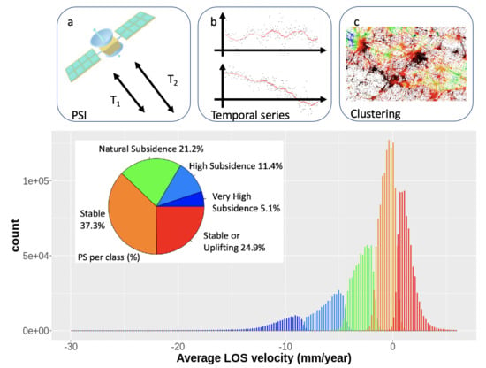
The aim of this work is presenting a methodology for the structural health monitoring of underground infrastructures. Our approach is based on three distinct steps: (a) collection of remote sensing data for Persistent Scatterer Interferometry; (b) study of temporal series terrain deformations; and, (c) unsupervised clustering for detection of similarity patterns. An outline of the proposed approach is presented in
Figure 1.
In particular, we examined the case of the underground aqueduct network of the Italian provinces of Modena and Bologna. This network consists of 58,392 georeferenced segments that were described by a set of 27 variables accounting for technical properties, like the material or the diameter, or geographical information, like the related municipality; although some of these features could be relevant for this study, we did not consider any of them to keep our approach based as much as possible on the sole PSI. For 47 aqueduct stretches it is also known if any maintenance was required after the observation time, which ended in 2019. Thus, while using this ground truth, we were also able to evaluate the accuracy of the proposed approach.
2.1. PSI Analysis
In this work, we used Sentinel-1 C-band images (central frequency
GHz and wavelength
cm), covering the Northern Italy and, in particular, the Bologna and Modena provinces, see
Figure 2.
The Sentinel-1 constellation is currently composed of two twin satellites (Sentinel-1A and Sentinel-1B, respectively); the first one is active from October 2014 and the second one from September 2017, they observe the Earth from an altitude of about 693 km, at a nominal ground resolution of about m2 (range × azimuth) and with a revisit time of 6 days at the equator. The study area is covered along two satellite tracks, in both ascending and descending geometries; in order to estimate the terrain movements, we used ascending observations from 30 March 2015 to 24 January 2019 and descending ones from 12 October 2014 to 25 January 2019 corresponding to 180 and 185 acquisitions, respectively. The ascending orbit consisted of ∼3.0 observations while for the descending orbit we had ∼3.9 observations; for both geometries the additional information about the Digital Elevation Model, latitude and longitude, coherence, head angle and incident angle were also available. We separately used the two geometries for two reasons: (i) the combination of ascending and descending orbit cause loss of spatial resolution; and, (ii) the combination of different geometries may hide inhomogeneous movements.
We used the SPINUA (Stable Point INterferometry even over Un-urbanised Areas) processing chain [
15] to evaluate terrain displacements. PSI are well-established methods that are based on the processing of temporal series of co-registered SAR images acquired over the same target area. The main idea of PSI is that terrain movements can be derived by phase-shift differences, thus identifying a grid of movements for point-like targets (corresponding to single pixels) usually referred as Persistent Scatterers (PS). An important aspect of these measures is their phase coherence over the entire observation period; in fact, it is possible to assess the coherence with dedicated statistical analyses and neglect those measures, which do not reach a satisfactory value. For the present analyses, we selected the time-series whose phase coherence exceeded the
threshold value [
16], which ensures, in this case, an RMSE below 4 mm, for each displacement measurement.
There is another class of measurement points that can be extracted by using the SPINUA processing chain, they are named Distributed Scatterers (DS) and are coherent measurements obtained by spatial averaging statistical homogeneous pixels. The use of groups of pixels in the case of DS is dictated by the need to operate spatial averages between adjacent pixels of the same nature in order to reduce the presence of noise. This technique is particularly useful in order to extract measurement points in non-urban areas, i.e., arid areas with low vegetation and debris. On the contrary, in the case of the PS, the target inside the single pixel is sufficiently dominant with regard to the noise and, therefore, it is not necessary to further improve the quality of the phase response; this also allows for preserving the maximum spatial resolution of the target itself. In the case of DS, instead, spatial average operations introduce an unavoidable spatial resolution loss compared to the native resolution of the radar image. For that reason, only measurements derived from point-like targets have been taken into account in the present work, see
Appendix A for further details.
The time series obtained for each PS within the examined grid were then clusterized with the k-means algorithm; the backbone of our approach consists in detecting similar patterns of PS and then grouping them together.
2.2. K-Means Clustering
Clustering techniques are unsupervised learning methods that basically exploit the informative content provided by the descriptive features of a dataset to outline the presence of similarities between different observations. Clustering techniques are divided into hierarchical and partitioning. The main advantage of hierarchical algorithms is that the number of the clusters directly emerges from data. However, these algorithms have a quadratic computational complexity [
17,
18], which restricts their application to small sets of data. This is why we used a partitioning algorithm with a linear computational complexity, like k-means.
In the k-means algorithm [
19,
20], the initial step consists in randomly setting
N points, called centroids, whose number is equal to number of clusters that the data will be partitioned in. Of course, this is a parameter that needs to be tuned. For each cluster
, the centroid
is defined as the mean value of all observations
assigned to the cluster:
The choice to assign an observation to a specific cluster is taken by the minimization of a cost function
:
which is the sum of the squared Euclidean distances between the objects
end their centers
.
Table 1 outlines the iterative procedure adopted to minimize the function of cost
W.
The main drawback of k-means is that its partitioning is strongly affected by the random initialization of centroids. For this reason, we performed 10,000 repetitions and averaged their results in order to obtain our final partition. Finally, as the examined time series consist of terrain displacements over time, the patterns detected by k-means can physically be interpreted as group of PS moving with the same velocity of the cluster centroid.
We explored a number of k clusters varying from 2 to 10. To evaluate the clusters’ separation, we used three distinct indicators:
the between-sum-of-squares/total-sum-of-squares ratio ();
the Adjusted Rand Index (); and,
the Silhouette statistics S.
The
ratio basically compares the distance of points within a class with all the distances in the data; the
ratio ranges from 0 (perfect overlap) to 1 (disjoint clusters). The ARI indicator is a measure of agreement between two partitions of the same dataset. It is used here in order to measure the agreement between different k-means initializations. The ARI indicator ranges from
to 1. Perfect agreement corresponds to 1, when
the agreement can be considered to be a random occurrence, while
denotes a perfect disagreement of the clusters. Finally, the silhouette
S measures the clustering consistency, in general a good experimental value should lie around
, further details and references regarding these metrics are presented in
Appendix B.
Once each PS within the observation grid was assigned to a cluster, we were able to detect critical areas.
2.3. Detection of Critical Areas
The underlying hypothesis of our approach consists in assuming that terrain deformations stress underground infrastructures, eventually causing severe damages or disruptions that require maintenance. Accordingly, we use the clustering analysis to detect which are the most probable regions where these phenomena can occur. In this work, we examined two distinct situations. On one hand, it is reasonable to assume that aqueduct stretches whose ends lie in different clusters; therefore, moving with different velocities will be subject to tension forces and frictions which account for the measured velocity difference and could yield infrastructural damages. This approach basically consists in determining a spatial gradient. On the other hand, even if the ends of a stretch belong to the same cluster, it is possible that the stretch experiences tensions and frictions, for example, because its central part lies in a region moving with different velocity; a figurative representation is shown in
Figure 3.
The latter case presents infinite possibilities to examine; nevertheless, we can model the problem with a slight change of perspective. Instead of focusing on the aqueduct stretch, we consider a region surrounding the stretch, which we name buffer, and compute this region purity in terms of the number of PS falling into this region and the number of different clusters they belong to.
Let us examine in detail the gradient approach. Once the PS have been assigned to a cluster we have a grid of labeled points over the region of interest. As previously mentioned, physically we can interpret this map as a discrete velocity field. In order to obtain a continuous velocity field, the most adopted choice would be the kriging method [
21], but the computational requirements suggested us an alternative strategy. Here, we used another consolidated interpolation procedure, the inverse distance weighting (IDW) interpolation [
22]. Given a set of discrete observations
with
, it is possible to define the interpolating function
, such that:
where
is a similarity function usually dependent on the reciprocal of a distance, as:
where
is the
i-th observation and
is its distance from
. In this study we adopted
to shorten the spatial influence of the measured grid. Finally, the gradients
and
of the interpolated field
f along the
x and
y directions were estimated with a
Sobel filter. In fact, we observed that, with a
filter, the edges appeared affected by a salt-and-pepper-like noise, while greater windows did not yield any improvement in both the image quality or in computational times.
Finally, the magnitude of the gradient
is computed, as follows:
The status of the segments of the water-supply network is then considered to require an inspection for maintenance by comparing the gradient value with a threshold .
For what concerns the buffer approach, the initial step, analogously to what we did with the gradient approach, consists in considering the PS clustering. In this case, there is no need for spatial interpolation, as we are only interested in evaluating the PS near an aqueduct stretch. To gain statistical robustness, we observed that a consistent number of PS was obtained for each stretch if we considered a buffer area (centered on the aqueduct stretch) having a 30 m radius. We considered the distribution of PS velocities within the buffer area and determined their variance, as a measure of homogeneity, the less the variance the greater the homogeneity; therefore, a critical aqueduct stretch was pointed out when the variance exceeded a threshold value .
It is worth noting that both the gradient and buffer approaches yield a score that can easily be interpreted as a classification score; in fact, the gradient itself and the variance within the buffer region can be thresholded, using and , respectively, resulting in a binary response about the aqueduct stretch, damaged or not. It is important to note, to underline the clustering robustness, that these thresholds affect the classification of the aqueduct stretch, not the k-means partitioning. These thresholds could be tuned according to several different considerations, in particular, as maintenance inspections are usually expensive both in terms of time and cost, we needed to consider the trade-off between the possibility to deliver warnings when maintenance was unnecessary (false positives) and neglect critical situations (false negatives); in other situations, for example, when large databases are available both for validation and testing accordingly, which is not the case here, these thresholds could be tuned according to classification performance. Thus, as performance metrics, we used in this work the Area Under the receiver operating characteristic Curve (AUC), which does not depend on the choice of a specific threshold value.
3. Results
3.1. How Many PS Patterns?
Our first analysis aimed at detecting how many distinct PS patterns could be detected in the region of interests.
Figure 4 shows the comparison of the BSS/TSS ratio and the ARI for ascending orbit.
We found that the BSS/TSS ratio reached the higher values from a number of clusters
; on the contrary, the ARI showed the best separation of clusters when
. Therefore, these two metrics would suggest using
. Besides, we investigated the silhouette
S, for
, we found
. We also observed that, except the case
showing
, according to the silhouette metrics all the examined
k values show a good consistency (
).
Figure 5 presents the results.
Therefore, the subsequent analyses were performed when considering 5 different clusters. It should be noted that, when repeating the analysis with the descending geometry, we obtained the same result.
3.2. The Physical Interpretation of Clusters
An indirect validation of the previous result about the number of detected PS patterns was obtained by inspecting the distribution of the average line of sight (LOS) velocities within each cluster, see
Figure 6.
We estimated the velocity of each PS in a cluster and therefore the cluster velocity distribution. We observed a nice separation for these distributions, so that it was possible to consider each cluster physically associated to a well-defined terrain movement in terms of average cluster velocity: “very high subsidence” (
mm/year), “high subsidence” (
mm/year), “natural subsidence” (
mm/year), “stable” (
mm/year), and “stable or uplifting” (
mm/year).
Figure 6 also shows the percentage of PS points belonging to each cluster.
A visual inspection of the region of interest shows that the clusters have typical dimensions of about 2∼10 km, see
Figure 7.
All of the detected patterns have in general a spatial coherence so that it is difficult, for example, to find an uplifting region whose edges border on a very high subsidence region. Interestingly, at small regions (<1 km) a substantial inhomogeneity emerges, in these small regions is not unusual to find PS belonging even to 3 or 4 different classes.
3.3. Damage Detection on Underground Aqueduct Stretches
In order to validate our pipeline, we collected and examined 47 on field assessments provided by human experts. These evaluations showed in 44 cases the presence of a structural damage while in 3 cases there was no manifest need of intervention.
Figure 8 presents the predictions obtained while using the ascending orbit data.
Both the gradient and buffer methods performed better than chance with AUC
and AUC
, respectively. The reported standard error was calculated with the Hanley formula [
23]. At the operating points, the gradient method returned sensitivity
and specificity
while we obtained sensitivity
and specificity
for the buffer method.
According to a z-test, no significant difference can be detected between the two methods. A magnified view of a subsidence region with a detected damage is presented in
Figure 9.
3.4. Replication Study on the Descending Orbit
We repeated our classification analyses with the descending orbit data in order to confirm the robustness of the performed analyses and the performance accuracy, especially for the damage detection, see
Figure 10.
Even in this case, we observed no significant difference between the two approaches with a z-test. The same conclusions hold for a comparison between the descending orbit and ascending orbit results.
4. Discussion
The analyses determining the optimal number of clusters were entirely based on the concepts of stability and reproducibility; accordingly, we explored three different metrics: BSS/TSS ratio, ARI and silhouette
S. While BSS/TSS and ARI suggested that the best choice consisted in 5 clusters the
S best value was obtained for
. However, it is worth noting that
S values for all partitions were ≥0.45, which means that the clusters are consistent, even if there is not a huge separation. These results suggest that a separation based only on PSI data can be affected by a considerable uncertainty; time series covering a wider temporal range or dedicated methodologies could, in principle, improve the clustering results [
24,
25,
26]. Nevertheless, it is worth noting that, despite 10,000 different initializations, the clusters remained stable and their classification results reproducible while using two distinct datasets, the ascending and the descending geometries.
The clusters that were detected from our analysis have a nice physical validation. By inspecting the distribution velocities within each class, we found that each cluster could be characterized by a different LOS velocity. This is somehow expected, in that a reasonable clustering result should detect different terrain movements. In particular, we found that using the two available geometries, the optimal number of classes, 5, remained unchanged; this should not be taken for granted considering that the presence of horizontal (East-West) displacements can significantly change the LOS measurements obtained with the two geometries. In this regard, it must be considered that the region of interest is affected by tectonic motions in the NE direction (with velocity ranging from 3 mm/year to 6 mm/year) [
27,
28] which can yield significant changes to estimated velocities [
29]. This could explain the different average within-cluster LOS velocities obtained in the two geometries.
Finally, we have designed two different approaches, the gradient and the buffer methods, to evaluate whether terrain movements estimated by PSI can predict structural damages. We evaluated the classification accuracy of these methods while using a labeled dataset of maintenance interventions on the aqueduct stretches of the Italian provinces of Bologna and Modena, Northern Italy. We had 47 maintenance interventions by human experts that evaluated the presence or the absence of a structural damage on an underground aqueduct stretch. The overall accuracy in terms of AUC was higher than for both methods and for both ascending and descending orbit data. Our findings were statistically indistinguishable.
Despite the good level of accuracy, there are some critical aspects that should be taken into account: first of all, the limited size of labeled data; this prevents us from obtaining more precise estimates of the accuracy, in fact the standard errors obtained using the Hanley formula are –. Another aspect to be considered concerns the classification errors that can affect this kind of analysis. In general, classification errors are of two type, false positives and false negative. A performance analysis in terms of sensitivity and specificity showed how, despite an analogous classification performance, the two proposed methods have completely different behaviors, while the gradient is more accurate for the detection of not damaged stretches, the buffer on the contrary is more accurate for the damage detection. Future studies could address the possibility to combine these approaches and even improve the classification performance. In this analysis, we only examined the terrain movements as a possible cause of structural damage, but, of course, this is an oversimplification. Neglecting other possible damage causes affects the methodology preventing the detection of damages which therefore are false negatives. At the same time, the frictions and forces developed by in-homogeneous terrain movements can yield micro-damages which are not detected by human experts at the present but can accumulate over time eventually ending with an overt structural damage; these situation represent the false positives of this analysis. Based on these considerations, we are aware that the estimated AUC should be considered cum grano salis; nevertheless, our findings suggest that a structural health monitoring of underground infrastructures could be founded on PSI analyses.
As previously mentioned, the presented results would benefit from a larger labeled dataset. Another possible improvement concerns data resolution. Sentinel-1 resolution is adequate for the detection of the pipelines that are subject to ground motion, as the PS resolution ( m2) matches the typical dimensions of aqueduct stretches and reduces the regions to monitor, a fundamental aspect for operative requirements. In principle, high-resolution data (like Cosmo-SkyMed and TerraSAR-X) could improve the methodology. However, in Italy, these missions cannot ensure the systematic global coverage and the same revisit time provided by Sentinel-1; despite these limitations, future studies should evaluate to which extent high-resolution data can improve the proposed approach.
Finally, it could be of fundamental importance to design a framework of analysis that is able to manage heterogeneous data, not only from PSI, to take into account damages from other sources. With this regard, we aim at collecting more data and develop alternative strategies exploiting supervised learning [
30,
31,
32,
33]. In particular, novel graph-based approaches [
34,
35] and deep learning strategies [
36,
37,
38] seem to be able to bring significant advances to the field. These approaches are naturally suited to manage large and heterogeneous datasets, therefore they could represent the best options to improve the findings that are presented in this work and pave the way for future applications in underground SHM.
5. Conclusions
In this work, we proposed a PSI processing pipeline for the monitoring and automated detection of underground infrastructural damages, specifically we investigated the case of aqueduct stretches in the Italian provinces of Bologna and Modena, Northern Italy. Based on the well-established analysis techniques of PSI and unsupervised clustering k-means, the proposed approach detects coherent PS movements and clusters them in groups whose physical interpretation is given in terms of similar LOS velocity. The border regions between different clusters and the small inhomogeneous regions that include PS of from different clusters are considered potentially dangerous for infrastructures; in these regions, the frictions and forces that arise from the different terrain velocities can weaken the structural health of the aqueduct stretches. The proposed approach exploits the Sentinel-1 data. The use of high-resolution data or the combination of PSI with in situ measures could represent a great opportunity to further improve the reliability of the methodology; however, the method attested an accuracy in terms of AUC . Besides, it should not be underestimated the fact that, the current high-resolution missions have two major drawbacks related to (i) the economic cost of the data, that in some cases can be difficult to afford and (ii) the reduced spatial coverage capability, which prevents a systematic acquisition of data with global coverage and with a short revisit time, as instead happens with the Sentinel-1 mission. The reported performance can be largely affected by other factors, such as an increment of the available data. An intrinsic and unavoidable limitation is caused by the presence of damages that are caused by other sources and the damages whose signals cannot be detected from the proposed approach. Nevertheless, we demonstrated that the proposed approach is able to detect the relation between terrain movements and underground structural damages.
Author Contributions
Conceptualization, N.A. and R.C. and A.T. and A.M.; methodology, N.A. and R.C.; software, R.C.; formal analysis, R.C.; writing—original draft preparation, N.A.; writing—review and editing, N.A., R.C., L.B., A.T., V.M., A.M., D.O.N., R.N., S.S., N.T., S.T., A.T., L.G. and R.B.; visualization, N.A.; supervision, N.A. and R.B.; funding acquisition, R.B. All authors have read and agreed to the published version of the manuscript.
Funding
This research received no external funding.
Acknowledgments
Authors would like to thank IT resources made available by ReCaS, a project funded by the MIUR (Italian Ministry for Education, University and Re-search) in the “PON Ricerca e Competitività 2007–2013-Azione I-Interventi di rafforzamento strutturale” PONa3_00052, Avviso 254/Ric, University of Bari. This paper has been supported by the DECiSION (Data-drivEn Customer Service InnovatiON) project co-funded by the Apulian INNONETWORK program.
Conflicts of Interest
The authors declare no conflict of interest.
Appendix A. Displacement Maps
PSI is used to create the displacement maps used in this work. More specifically,
Figure A1 shows results obtained SPINUA for the ascending geometry.
The visualization has been performed by using Rheticus
® Displacement, which is a cloud-based operational service based on the SPINUA algorithm and designed for monitoring ground surface movements through Multi-Temporal SAR Interferometry analyses [
39]. An analogous result is presented in
Figure A2 for the descending orbit.
Figure A1.
The displacement map obtained for the ascending orbit.
Figure A1.
The displacement map obtained for the ascending orbit.
The region of interest is affected by well-known subsidence phenomena, thus, is reasonable to assume that these motions could affect the structural health of the aqueduct stretches. Besides, subsidence phenomena could help to understand the presence of possible deformations in areas not covered by PSI data.
In particular, we compared the PSI clustering map with the geological environment of the metropolitan area of Bologna. This region can be divided in several regions, usually called conoids, composed of unconsolidated sediments (mainly gravel and sand); three different areas can be detected within the region of interest: the alluvial plain, the Reno-Lavino and the Savena alluvial conoids; in particular, the two alluvial conoids are usually divided in two different conoids according to their different cinematic properties. The comparison is shown in
Figure A3.
Figure A2.
The displacement map obtained for the descending orbit.
Figure A2.
The displacement map obtained for the descending orbit.
Figure A3.
The left panel shows the five clusters retrieved by the PSI analysis corresponding to very high subsidence (blue), subsidence (light blue), natural subsidence (green), stable (orange), stable/uplifting (red). The right panel shows the geological map of the Bologna-Modena region divided in alluvial plain (purple), northern and southern Reno-Lavino alluvial conoids (blue and red, respectively) and northern and southern conoids (green and light red, respectively).
Appendix B. Metrics for Cluster Stability
The BSS/TSS ratio is defined as ratio between the sum of distances
between couples of objects belonging to different clusters and the sum of distances
T between all the couples of objects belonging to the whole dataset:
The values of the BSS/TSS ratio measures the separation between the output clusters and ranges between 0 and 1. These values correspond to, respectively, perfectly overlapped cluster (worst scenario) and to point-like clusters that result perfectly separated.
It is useful to estimate if the output of the resulting clustering appears to be dependent to the random initialization of kmeans algorithm. In order to do so, we considered the adjusted Rand Index (ARI) as an internal validation metrics. Let be
and
two clustering segmentation in
K classes of the same dataset
D. For these clustering it is possible to define the related contingency matrix:
where
is the number of objects that belong to
,
is the number of objects that belong to
and
is the number of objects that belong to
. With respect to this context, the ARI metrics is defined as follow:
As the definition of the ARI is not straightforward, we suggest to interpret (
A3) as the relative number of couples of labels from two clustering
and
in mutual agreement. The ARI metrics ranges between 1 and
, with 1 corresponding to perfect mutual agreement,
corresponding to perfect disagreement and 0 that correspond to random agreement between the two clusters.
A consistency measure of clusters is by the Silhouette statistics
S. Let us define the similarity
of the
i-th object belonging to
with respect to the remaining objects that belong to the same cluster
as:
Similarly, it is possible to introduce the dissimilarity
between the
i-th object in
and any objects that does not belong to
as follows:
The Silhouette statistics
of the
i-th object is defined as the the ratio:
The above statistics ranges between and 1. Values of close to 1 show that the i-th objects in is highly dissimilar with respect to the objects from the other clusters . Conversely, a value close to zero or negative shows that the i-th object is very dissimilar to the objects that belong to the same cluster.
Finally, it is possible to define the average Silhouette statistics as:
As it could be expected, the average Silhouette values ranges between 0 and 1. Kaufman and Rousseeuw [
40] claim that a clustering should be retained as valid if
and invalid if
. We computed the average Silhouette statistics over a uniform sample of 10,000 measurement points.
References
- Aktan, A.; Helmicki, A.; Hunt, V. Issues in health monitoring for intelligent infrastructure. Smart Mater. Struct. 1998, 7, 674. [Google Scholar] [CrossRef]
- Bhalla, S.; Yang, Y.; Zhao, J.; Soh, C. Structural health monitoring of underground facilities—Technological issues and challenges. Tunn. Undergr. Space Technol. 2005, 20, 487–500. [Google Scholar] [CrossRef]
- Jo, B.W.; Khan, R.M.A.; Lee, Y.S. Hybrid blockchain and internet-of-things network for underground structure health monitoring. Sensors 2018, 18, 4268. [Google Scholar] [CrossRef] [PubMed] [Green Version]
- Liu, Z.; Liu, P.; Zhou, C.; Huang, Y.; Zhang, L. Structural Health Monitoring of Underground Structures in Reclamation Area Using Fiber Bragg Grating Sensors. Sensors 2019, 19, 2849. [Google Scholar] [CrossRef] [PubMed] [Green Version]
- Qian, Q.; Lin, P. Safety risk management of underground engineering in China: Progress, challenges and strategies. J. Rock Mech. Geotech. Eng. 2016, 8, 423–442. [Google Scholar] [CrossRef] [Green Version]
- Strozzi, T.; Delaloye, R.; Poffet, D.; Hansmann, J.; Loew, S. Surface subsidence and uplift above a headrace tunnel in metamorphic basement rocks of the Swiss Alps as detected by satellite SAR interferometry. Remote Sens. Environ. 2011, 115, 1353–1360. [Google Scholar] [CrossRef] [Green Version]
- Fornaro, G.; Reale, D.; Verde, S. Bridge thermal dilation monitoring with millimeter sensitivity via multidimensional SAR imaging. IEEE Geosci. Remote Sens. Lett. 2012, 10, 677–681. [Google Scholar] [CrossRef]
- Milillo, P.; Giardina, G.; DeJong, M.J.; Perissin, D.; Milillo, G. Multi-temporal InSAR structural damage assessment: The London crossrail case study. Remote Sens. 2018, 10, 287. [Google Scholar] [CrossRef] [Green Version]
- Scaioni, M.; Marsella, M.; Crosetto, M.; Tornatore, V.; Wang, J. Geodetic and remote-sensing sensors for dam deformation monitoring. Sensors 2018, 18, 3682. [Google Scholar] [CrossRef] [Green Version]
- Corsetti, M.; Fossati, F.; Manunta, M.; Marsella, M. Advanced SBAS-DInSAR technique for controlling large civil infrastructures: An application to the Genzano di Lucania dam. Sensors 2018, 18, 2371. [Google Scholar] [CrossRef] [Green Version]
- Özer, I.E.; van Leijen, F.J.; Jonkman, S.N.; Hanssen, R.F. Applicability of satellite radar imaging to monitor the conditions of levees. J. Flood Risk Manag. 2019, 12, e12509. [Google Scholar] [CrossRef] [Green Version]
- Milillo, P.; Giardina, G.; Perissin, D.; Milillo, G.; Coletta, A.; Terranova, C. Pre-collapse space geodetic observations of critical infrastructure: The Morandi bridge, Genoa, Italy. Remote Sens. 2019, 11, 1403. [Google Scholar] [CrossRef] [Green Version]
- Bitelli, G.; Bonsignore, F.; Unguendoli, M. Levelling and GPS networks to monitor ground subsidence in the Southern Po Valley. J. Geodyn. 2000, 30, 355–369. [Google Scholar] [CrossRef]
- Marchetti, M. Environmental changes in the central Po Plain (northern Italy) due to fluvial modifications and anthropogenic activities. Geomorphology 2002, 44, 361–373. [Google Scholar] [CrossRef]
- Bovenga, F.; Refice, A.; Nutricato, R.; Guerriero, L.; Chiaradia, M. SPINUA: A flexible processing chain for ERS/ENVISAT long term interferometry. In Proceedings of the ESA-ENVISAT Symposium, Salzburg, Austria, 6–10 September 2005; pp. 6–10. [Google Scholar]
- Ferretti, A.; Prati, C.; Rocca, F. Permanent scatterers in SAR interferometry. IEEE Trans. Geosci. Remote Sens. 2001, 39, 8–20. [Google Scholar] [CrossRef]
- Murtagh, F.; Contreras, P. Algorithms for hierarchical clustering: An overview. Wiley Interdisc. Rew. Data Min. Knowl. Discov. 2012, 2, 86–97. [Google Scholar] [CrossRef]
- Murtagh, F. A Survey of Recent Advances in Hierarchical Clustering Algorithms. Comput. J. 1983, 26, 354–359. [Google Scholar] [CrossRef] [Green Version]
- Lloyd, S. Least squares quantization in PCM. IEEE Trans. Inf. Theory 1982, 28, 129–137. [Google Scholar] [CrossRef]
- MacQueen, J. Some methods for classification and analysis of multivariate observations. In Proceedings of the Fifth Berkeley Symposium on Mathematical Statistics and Probability, Volume 1: Statistics; University of California Press: Berkeley, CA, USA, 1967; pp. 281–297. [Google Scholar]
- Cressie, N. The origins of kriging. Math. Geol. 1990, 22, 239–252. [Google Scholar] [CrossRef]
- Shepard, D. A Two-Dimensional Interpolation Function for Irregularly-Spaced Data. In Proceedings of the 1968 23rd ACM National Conference, ACM ’68; Association, for Computing Machinery: New York, NY, USA, 1968; pp. 517–524. [Google Scholar] [CrossRef]
- Hanley, J.A.; McNeil, B.J. The meaning and use of the area under a receiver operating characteristic (ROC) curve. Radiology 1982, 143, 29–36. [Google Scholar] [CrossRef] [Green Version]
- Liu, G.; Jia, H.; Zhang, R.; Zhang, H.; Jia, H.; Yu, B.; Sang, M. Exploration of subsidence estimation by persistent scatterer InSAR on time series of high resolution TerraSAR-X images. IEEE J. Sel. Top. Appl. Earth Obs. Remote Sens. 2010, 4, 159–170. [Google Scholar] [CrossRef]
- Cigna, F.; Bianchini, S.; Casagli, N. How to assess landslide activity and intensity with Persistent Scatterer Interferometry (PSI): The PSI-based matrix approach. Landslides 2013, 10, 267–283. [Google Scholar] [CrossRef] [Green Version]
- Scifoni, S.; Bonano, M.; Marsella, M.; Sonnessa, A.; Tagliafierro, V.; Manunta, M.; Lanari, R.; Ojha, C.; Sciotti, M. On the joint exploitation of long-term DInSAR time series and geological information for the investigation of ground settlements in the town of Roma (Italy). Remote Sens. Environ. 2016, 182, 113–127. [Google Scholar] [CrossRef]
- Baldi, P.; Casula, G.; Cenni, N.; Loddo, F.; Pesci, A. GPS-based monitoring of land subsidence in the Po Plain (Northern Italy). Earth Planet. Sci. Lett. 2009, 288, 204–212. [Google Scholar] [CrossRef]
- Baldi, P.; Casula, G.; Cenni, N.; Loddo, F.; Pesci, A.; Bacchetti, M. Vertical and horizontal crustal movements in Central and Northern Italy. Boll. Soc. Geol. Ital. 2011, 52. [Google Scholar] [CrossRef]
- Elliott, J.R.; Walters, R.J.; Wright, T.J. The role of space-based observation in understanding and responding to active tectonics and earthquakes. Nat. Commun. 2016, 7, 13844. [Google Scholar] [CrossRef] [Green Version]
- Ahmad, S.; Kalra, A.; Stephen, H. Estimating soil moisture using remote sensing data: A machine learning approach. Adv. Water Resour. 2010, 33, 69–80. [Google Scholar] [CrossRef]
- Lary, D.J.; Alavi, A.H.; Gandomi, A.H.; Walker, A.L. Machine learning in geosciences and remote sensing. Geosci. Front. 2016, 7, 3–10. [Google Scholar] [CrossRef] [Green Version]
- Maxwell, A.E.; Warner, T.A.; Fang, F. Implementation of machine-learning classification in remote sensing: An applied review. Int. J. Remote Sens. 2018, 39, 2784–2817. [Google Scholar] [CrossRef] [Green Version]
- Cilli, R.; Monaco, A.; Amoroso, N.; Tateo, A.; Tangaro, S.; Bellotti, R. Machine Learning for Cloud Detection of Globally Distributed Sentinel-2 Images. Remote Sens. 2020, 12, 2355. [Google Scholar] [CrossRef]
- Chaudhuri, B.; Demir, B.; Chaudhuri, S.; Bruzzone, L. Multilabel remote sensing image retrieval using a semisupervised graph-theoretic method. IEEE Trans. Geosci. Remote Sens. 2017, 56, 1144–1158. [Google Scholar] [CrossRef]
- Kong, Y.; Wang, X.; Cheng, Y. Spectral–spatial feature extraction for HSI classification based on supervised hypergraph and sample expanded CNN. IEEE J. Sel. Top. Appl. Earth Obs. Remote Sens. 2018, 11, 4128–4140. [Google Scholar] [CrossRef]
- Zhang, L.; Zhang, L.; Du, B. Deep learning for remote sensing data: A technical tutorial on the state of the art. IEEE Geosci. Remote Sens. Mag. 2016, 4, 22–40. [Google Scholar] [CrossRef]
- Zhu, X.X.; Tuia, D.; Mou, L.; Xia, G.S.; Zhang, L.; Xu, F.; Fraundorfer, F. Deep learning in remote sensing: A comprehensive review and list of resources. IEEE Geosci. Remote Sens. Mag. 2017, 5, 8–36. [Google Scholar] [CrossRef] [Green Version]
- Fu, G.; Liu, C.; Zhou, R.; Sun, T.; Zhang, Q. Classification for high resolution remote sensing imagery using a fully convolutional network. Remote Sens. 2017, 9, 498. [Google Scholar] [CrossRef] [Green Version]
- Samarelli, S.; Agrimano, L.; Epicoco, I.; Cafaro, M.; Nutricato, R.; Nitti, D.O.; Bovenga, F. Rheticus®: A Cloud-Based Geo-Information Service for Ground Instabilities Detection and Monitoring. In Proceedings of the IGARSS 2018–2018 IEEE International Geoscience and Remote Sensing Symposium, Valencia, Spain, 22–27 July 2018; pp. 2238–2240. [Google Scholar]
- Kaufman, L.; Rousseeuw, P.J. Finding Groups in Data: An Introduction to Cluster Analysis; John Wiley & Sons: Hoboken, NJ, USA, 2009; Volume 344. [Google Scholar]
| Publisher’s Note: MDPI stays neutral with regard to jurisdictional claims in published maps and institutional affiliations. |
© 2020 by the authors. Licensee MDPI, Basel, Switzerland. This article is an open access article distributed under the terms and conditions of the Creative Commons Attribution (CC BY) license (http://creativecommons.org/licenses/by/4.0/).

 ,
, 


