Article

Spatiotemporal Changes in 3D Building Density with LiDAR and GEOBIA: A City-Level Analysis

1
Department of Forest Resource Management, Faculty of Forestry, University of Agriculture in Krakow, 31-425 Krakow, Poland
2
Urban Development and Mobility Department, Luxembourg Institute of Socio-Economic Research, L-4366 Esch-sur-Alzette, Luxembourg
3
Urban Systems Lab, The New School, New York, NY 10003, USA
4
LEMA, Urban and Environmental Engineering Department, Liège University, 4000 Liège, Belgium
*
Author to whom correspondence should be addressed.
Remote Sens. 2020, 12(21), 3668; https://doi.org/10.3390/rs12213668
Submission received: 12 October 2020 / Revised: 1 November 2020 / Accepted: 6 November 2020 / Published: 9 November 2020
(This article belongs to the Special Issue Understanding Urban Systems Using Remote Sensing)

Abstract

:
Understanding how, where, and when a city is expanding can inform better ways to make our cities more resilient, sustainable, and equitable. This paper explores urban volumetry using the Building 3D Density Index (B3DI) in 2001, 2010, 2019, and quantifies changes in the volume of buildings and urban expansion in Luxembourg City over the last two decades. For this purpose, we use airborne laser scanning (ALS) point cloud (2019) and geographic object-based image analysis (GEOBIA) of aerial orthophotos (2001, 2010) to extract 3D models, footprints of buildings and calculate the volume of individual buildings and B3DI in the frame of a 100 × 100 m grid, at the level of parcels, districts, and city scale. Findings indicate that the B3DI has notably increased in the past 20 years from 0.77 m3/m2 (2001) to 0.9 m3/m2 (2010) to 1.09 m3/m2 (2019). Further, the increase in the volume of buildings between 2001–2019 was +16 million m3. The general trend of changes in the cubic capacity of buildings per resident shows a decrease from 522 m3/resident in 2001, to 460 m3/resident in 2019, which, with the simultaneous appearance of new buildings and fast population growth, represents the dynamic development of the city.

Graphical Abstract

1. Introduction

As the urban is extending, monitoring change over space and time is important for supporting decisions about appropriate development practices and land resource use. Increasing demands in urban management sectors need the coordinated use of remote sensing and a geographic information system (GIS) for monitoring urban intensification [1]. Building density is one of the most important indices for city monitoring [2]. Urban structure analyzes are carried out in two dimensions (2D), where building footprints are solely considered, or in three dimensions (3D), where building heights and footprints are considered [3]. However, in growing countries, obtaining accurate, complete, and current building information from cadastral data is hard to come by [4,5]. Two metrics often used in the regulations of city planning are the floor area ratio (FAR) and the building coverage ratio (BCR). FAR is the relationship of the gross floor area of a building to the total buildable area of the lot/parcel. BCR is calculated by dividing the total buildable area of a lot/parcel by the total area of the lot/parcel [6].
Remotely sensed imagery and GIS analysis are often used to extract building footprints. Various classification methods based on high-resolution satellite imagery have been used to derive the 2D building surface area [7,8,9,10] and landscape metrics [11,12]. One method of automatic image classification is the geographic object-based image analysis (GEOBIA) approach, which creates new spatial information within the GIS environment [13]. An object-based classification, based on groups of pixels, creates homogeneous and conceptually logical segments (objects) that reflect real-world entities more realistic than geometric systems of individual pixels [14,15]. This approach approximates algorithmic data processing to the way people perceive objects or spatial units, which makes it possible to create objects that are more intuitive during image segmentation [13]. GEOBIA enables the use of, besides spectral features, spatial features, such as height, shape, texture, surface, topology, relationships between segments, etc., forming the knowledge base [16]. The development of technologies such as LiDAR (Light Detection and Ranging) increases the usage of height models, i.e., the digital terrain model (DTM) and the digital surface model (DSM) in the city monitoring characterizing build-up areas. Currently, an increased number of cities offer open access to point clouds obtained from airborne laser scanning (ALS), so the next step is to implement buildings segmentation algorithms to generate shapes easy to process for future analysis. Therefore, recent studies are using data fusion of high-spatial resolution satellite imagery and DSM for building detection [17,18,19] and applying, for instance, neural networks [20,21].
Information about the geometry of buildings in 3D provides short- and long-term advantages for urban analysis [22]. Several studies focused on building height estimation using remotely sensed data via different methods, for example using building shadows [23,24], synthetic aperture radar (SAR) imagery [25,26,27] or stereo images matching [28]. Yet, many satellite sensors have limited detection capabilities; often, sensors can only estimate an average height, not including various roof parts heights, for each building [29]. Solid theoretical background for building height estimation and 3D reconstruction with roof structures provides LiDAR data [30]. A little research has been done for analyzing the 3D of urban structure, to develop spatial pattern metrics in landscape scale [31] and visualization of city model [32], which also have high potential for supporting the ‘smart city’ concept [33]. One of the most comprehensive research was carried out in 2020 by Li et al. [34], where random forest models were used to generate a map of urban 3D building structure at a continental scale (1 km2 spatial resolution). Wang et al. (2018) investigated fusion of Landsat images (L5, L8) and global DSMs data (SRTM, ASTER GDEM, AW3D30) to produce building height and volume maps (GSD 30 m) to the entire England using object-based and machine learning algorithms [35]. Additionally, EMU Analytics company made a “Building Heights in England” map, based on DTM and DSM too (open data from the Environment Agency for the UK) to explore how building density varies across the country in the top 25 urban cores in UK. They used local and open street maps for the building footprint and added the mean heights from nDSM to the buildings layer [36]. Krehl et al. (2016) calculated built-up volume in German City Regions using Cartosat-1 stereo images and the footprint of buildings [37]. Shirowzhan at al. (2019) presented 3D metrics for the assessment of an urban form and changes: ratio of volume change bases on DSM and mass or space index as the relation of the volume of buildings to the total volume of an assumed cube. However, to use these metrics, the LiDAR time series are needed [38].
In the Grand Duchy of Luxembourg, the rapid pace of economic development and population growth put pressure on the available land stock [39]. The population of Luxembourg has been increased by over 60% in the past three decades (from 379,300 to 626,108 inhabitants in 1990 and 2020, respectively). The Luxembourg city has experienced a population growth rate of 62% within the same period (from 75,800 to 122,273 inhabitants) [40]. According to recent population forecasts made by EUROSTAT, Luxembourg’s population will continue to grow, exceeding one million inhabitants by 2062. Although Luxembourg City provides public spatial data at the country level (opendata.lu), there is a lack of built-up volumetric studies for Luxembourg. The concepts of digitization and smart sustainable densification quoted by the State were the reason for choosing Luxembourg as a study area, with a focus on the capital of the country. Challenges related to urban densification, and particularly the impact on quality of life, ecological functions, and social acceptability, seem justified to be considered in this case. The question of buildings density is closely connected to urbanization and how cities may grow in the future. Thus, it is important to track the city over time and across space: how does the three-dimensional density of buildings evolve in Luxembourg City over time?
In this paper, we propose a 3D index to detect changes in building volume density in the last 20 years in Luxembourg City employing ALS LiDAR point cloud (2019) and GEOBIA approach of archival orthophoto maps (2001, 2010). Our analysis was supported by datasets collected from orthophotos during the last 20 years concerning demolish and newly constructed buildings. We process ALS classified point clouds to extract the points reflecting a rooftop surface and generate 3D models only for buildings class. A building’s volume density has been calculated for all buildings in the city including residential and non-residential categories. The detection of archival footprints of buildings was carried out using the object-based method. The complex integration of final datasets is unique in research and gives us very detailed information about the urban spatiotemporal (4D) changes, considering volume, vertical, and horizontal buildings’ changes.
Our methodology is general and can be applied to several cities when LiDAR data is available.
In this study, our key objectives are:
(1)
To automate 3D building modelling and object-based footprints of buildings extraction;
(2)
To define Building 3D Density Index (B3DI);
(3)
To quantify changes in volume density in Luxembourg City over the last two decades (between 2001, 2010, and 2019).

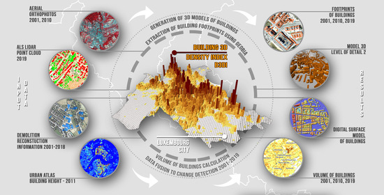
2. Materials and Methods

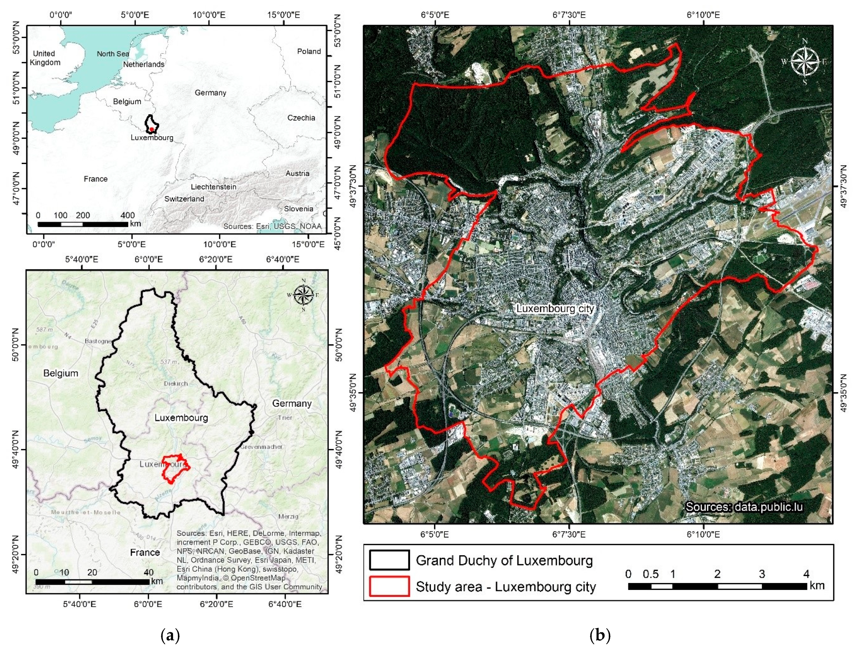
2.1. The Geographical Localisation of the Study Area

Luxembourg City is the capital of the Grand Duchy of Luxembourg and the country’s most populous city (Figure 1). Luxembourg City at municipality level occupies an area of 51 km2. The city has a complex topographic heterogeneous configuration, lying at the different levels with parks and forested areas. The city hosts several EU institutions, and it is one of the major international financial hubs. Changes in land use in Luxembourg in recent decades reveal a rapid urban development and land artificialization [41,42]. According to Corine Land Cover (CLC), made available by the European Environment Agency, urban land use in Luxembourg City covered about 35% and about 39% in 1990 and 2018, respectively. At the same time, the industrial, commercial, and transport uses increased by 3.3% whereas agricultural areas decreased by 6.6%, and forest and semi-natural areas decreased by 2.3%.

2.2. Datasets and Data Sources

In this study, we used ALS LiDAR point clouds from airborne mission obtained in February 2019 for Luxembourg City (mean point density was 15 points/m2 with horizontal and vertical accuracies was to ±3 cm and ±6 cm, respectively; in the area of the Luxembourg City, the average density was 25 points/m2) and archival RGB and CIR (color-infrared) aerial orthophoto maps from 2001, 2010, and 2019 (ground sampling distance (GSD) 50/25/20 cm), provided the Luxembourg Government’s open data (data.public.lu). The acquired point clouds were previously classified (ASPRS standard). The dataset was supplemented with cadastral information from 2019. However, the footprints of buildings were not updated and contained some errors in the geometries, thus, we generated footprints based on ALS LiDAR point cloud and added information about the use of buildings (residential or non-residential), according to cadastral data. We also used an archival database from the Housing Observatory of an on-going project [43,44] concerning the demolition/reconstruction (2001–2019) of buildings for Luxembourg, to detect buildings where there was a significant height change during the last two decades. This data was collected through the visual comparison of orthophotos every 3 years starting in 2001. To estimate the volume of buildings existing only in 2010, we acquired a layer of “Copernicus Urban Atlas—Building Height” from the European Environment Agency, within the framework of the Copernicus program. The product is a 10 m resolution and provides the height of buildings information that is generated for urban cores of capitals as part of the Urban Atlas project. Height information is based on IRS-P5 stereo images acquired as close as possible to the defined reference year and derived datasets like the digital surface model (DSM), the digital terrain model (DTM), and the normalized digital surface model (nDSM). Table 1 lists the data used in the current study.

2.3. Methods

Monitoring of spatiotemporal changes in the volume of buildings in Luxembourg City in 2001, 2010 and 2019 required integration of multi-source datasets and different methods of data analysis. This section presents a detailed description of all steps of analysis (Figure 2).

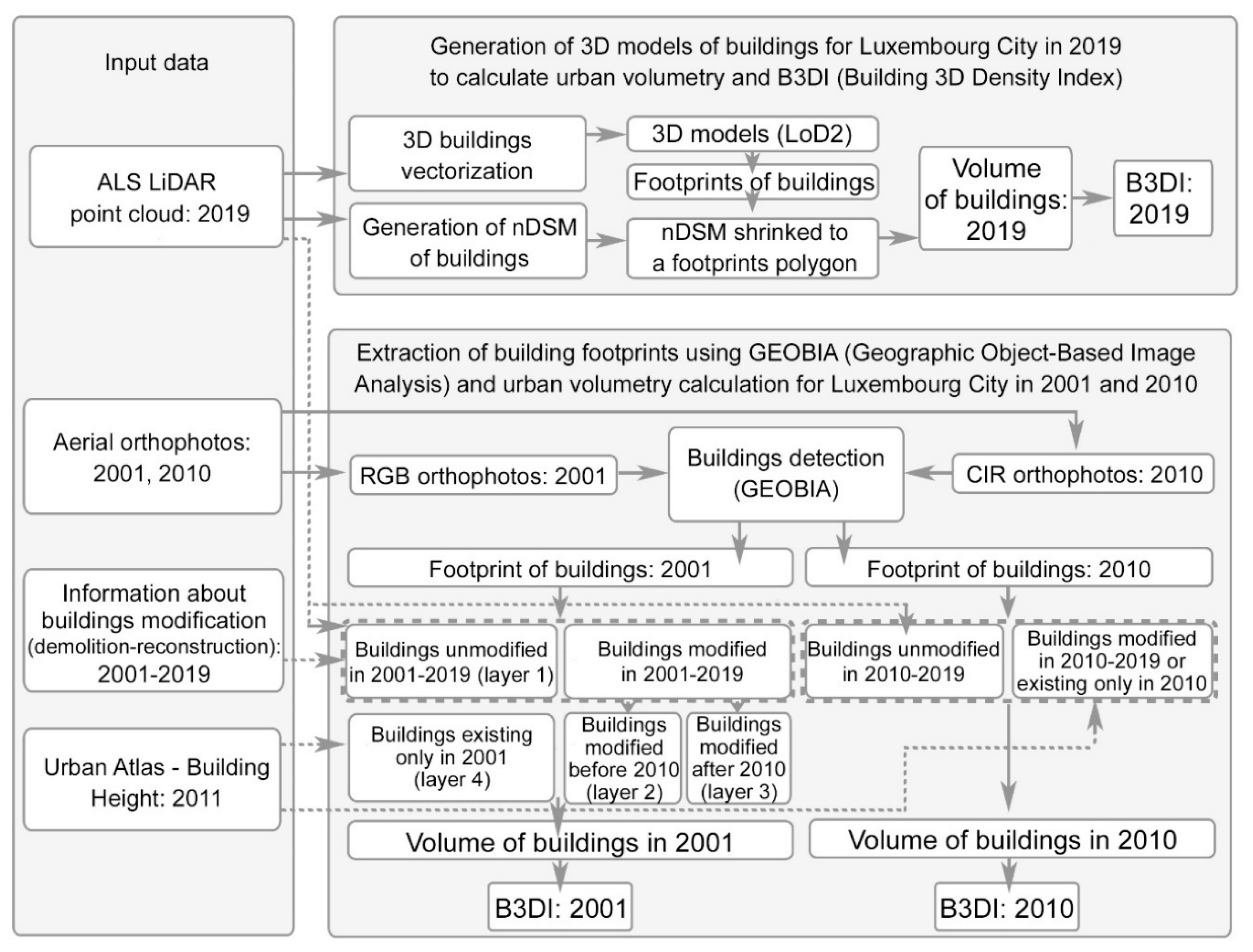
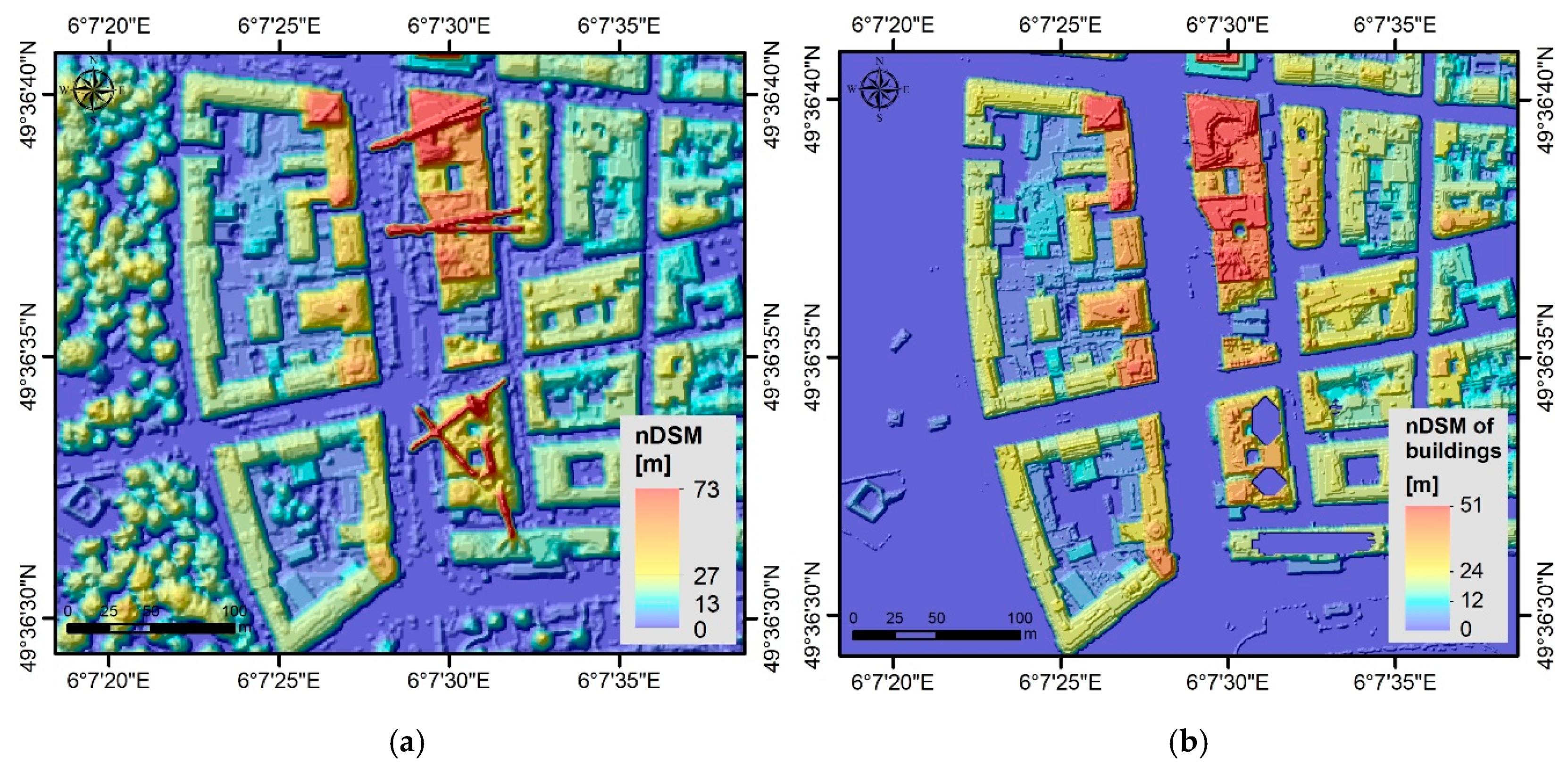
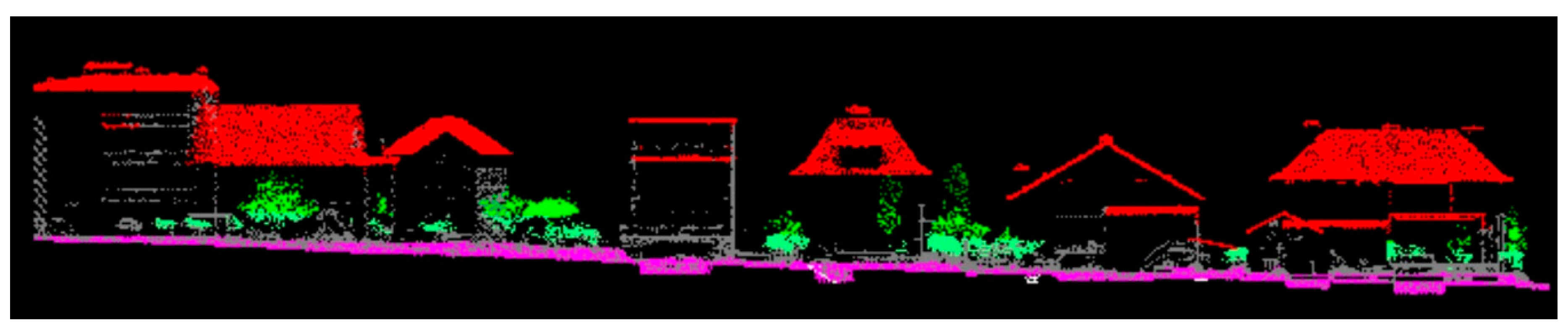
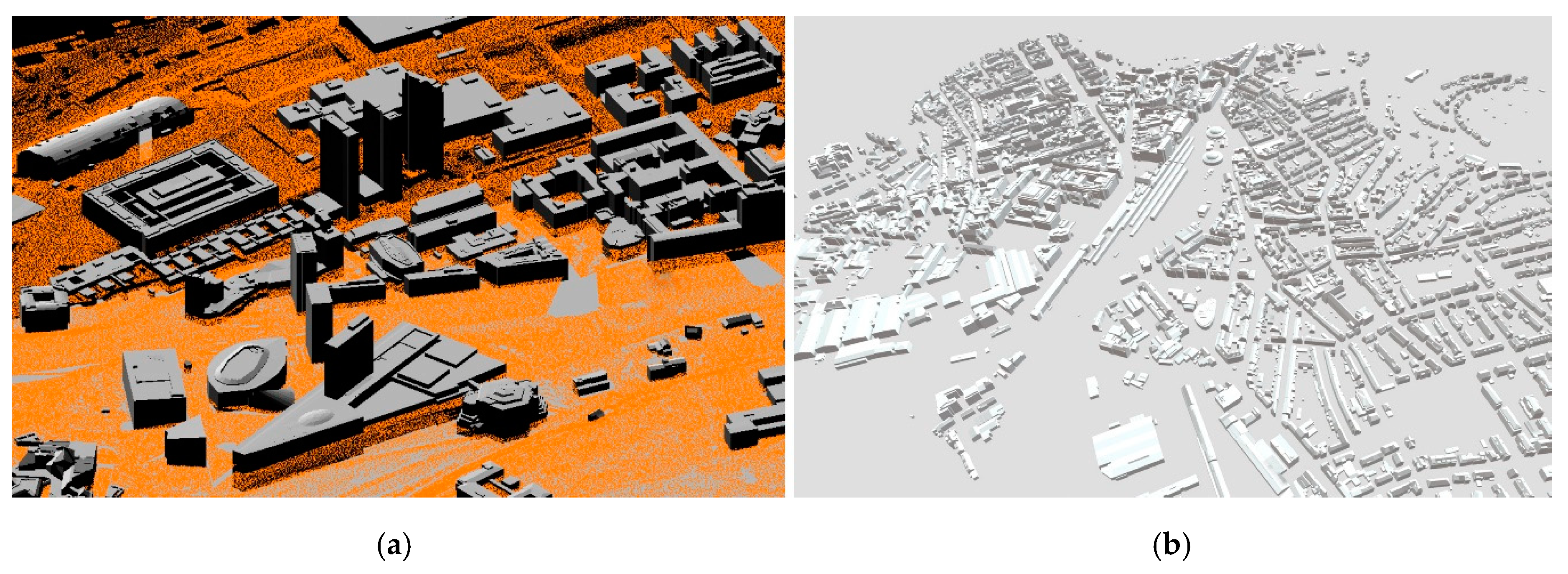
2.3.1. Generation of 3D Models of Buildings

ALS LiDAR point clouds were used to obtain precise information about the 3D configuration of the terrain and buildings in 2019. The processing was started by generating the DTM and the DSM of buildings from the classified point cloud (ASPR standard): class ground and building with 0.5 m resolution using Area Processor in FUSION software, ver. 3.70 (USDA Forest Service, Pacific Northwest Research Station). The nDSM, which represents the relative heights of buildings, was generated based on the difference of DSM and DTM rasters. The nDSM, generated from all classes of the point cloud, contains objects that could disturb the height or volume calculations of buildings (e.g., tree branches next to buildings or cranes on newly constructed buildings—example in Figure 3). For this reason, filtered nDSM, created only from buildings class, was used in further analysis.
Buildings vectorization was performed fully-automatically to generate non-planar roof shapes of buildings and 3D models of buildings in LoD2 (Level of Details; CityGML standard) based on classified ALS point clouds with two classes: ground and building (Figure 4) in TerraScan (Terrasolid) and MicroStation V8i (Bentley) software. These tools check and correct buildings’ topology. The quality of the automatic buildings’ vectorization depends not only on the quality of the LiDAR data processing that is done in preparation of the vectorization but also on the point density of the data. Based on 3D models, building footprints were generated and exported in the shapefile format. The minimum mapping area units (MMU) were 20 m2, and smaller objects were not included.
The nDSM of buildings (GSD 0.5 m) was shrunk to a roof polygon generated from ALS point cloud to eliminate errors on the height model. The model of buildings was used to determine the total volume of buildings [m3] and including the classification into residential and non-residential uses in Luxembourg City. The information about the category of buildings from cadastral data has been added to the shapefile of buildings in 2019. The volume of buildings was calculated for single buildings, at the districts-level and for standardization in cells (100 × 100 m) using ArcMap software (Esri) with the Zonal Statistics and Surface Volume tool, which calculates the volume of the region between a surface and a reference plane.

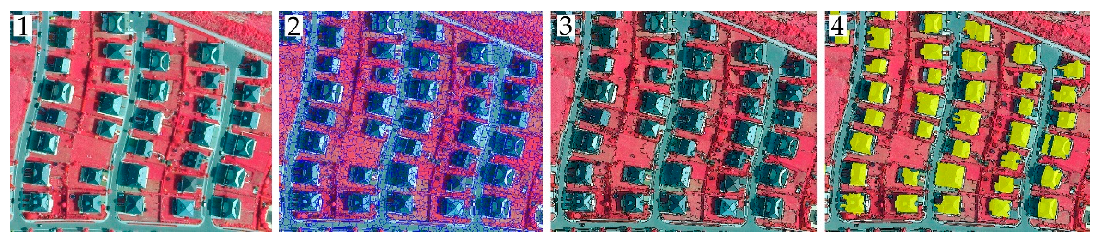
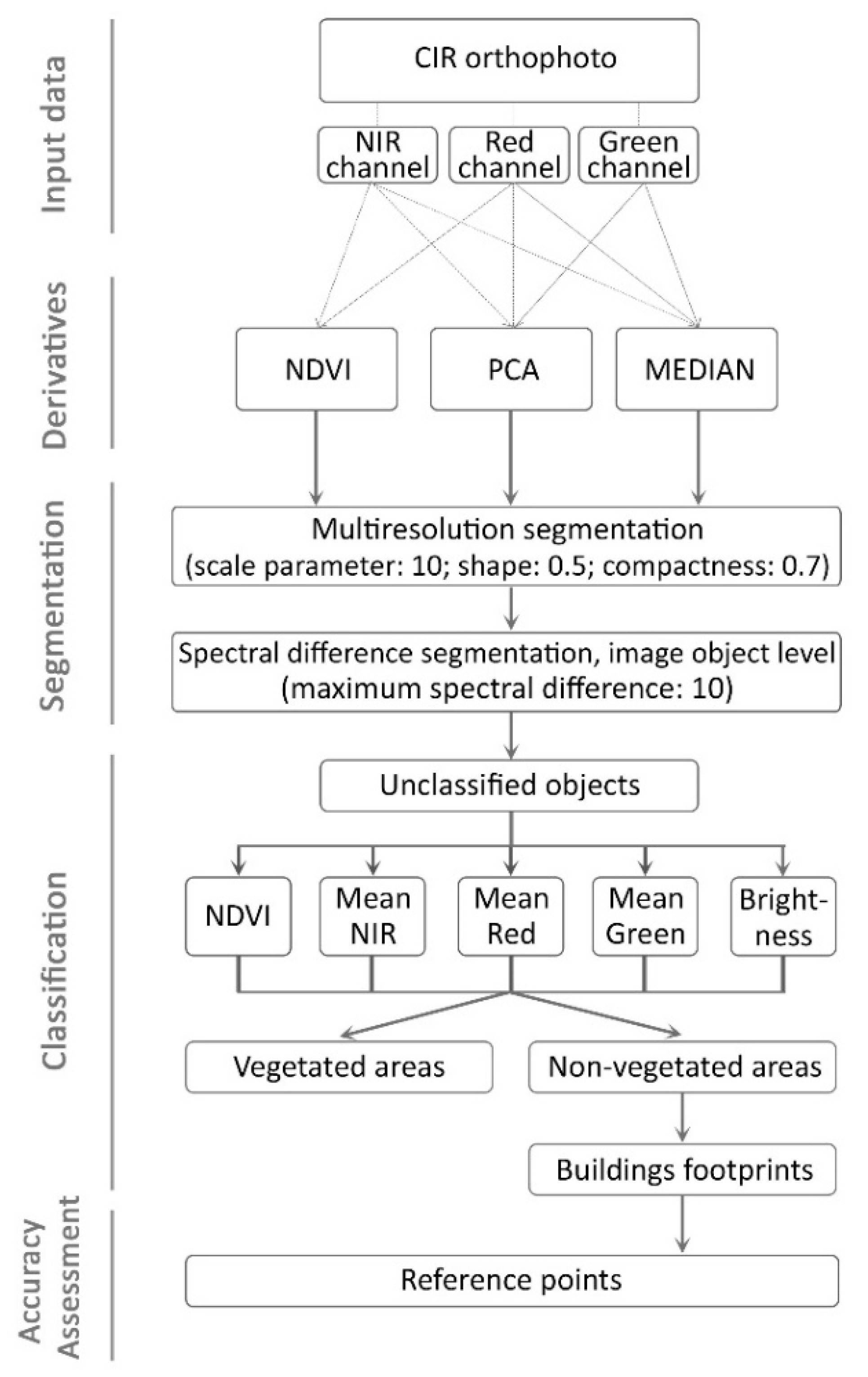
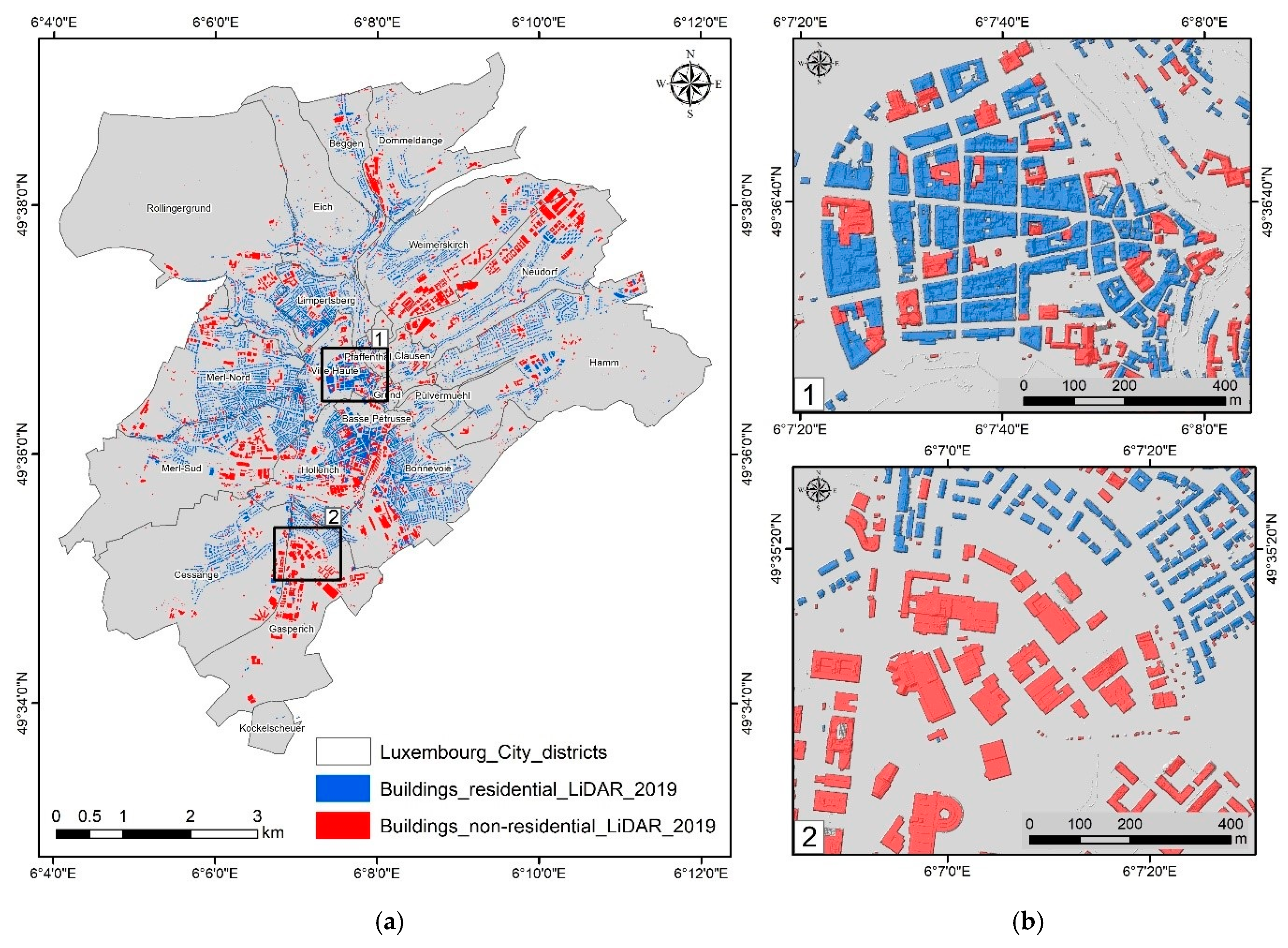
2.3.2. Extraction of Building Footprints Using GEOBIA and Volume Calculation

The object-based approach was applied to extract all buildings in Luxembourg City with RGB (2001, 2010) and CIR (2010) orthophoto maps using ruleset prepared in eCognition Developer 9.3 (Trimble Geospatial) software. The ruleset creation was started with generating the derivative layers based on spectral channels of CIR orthophotos. Using bands NIR (near-infrared) and Red, a normalized difference vegetation index (NDVI) layer was generated for separate areas with different spectral characteristics. In order to improve the contrast between the objects and the background and reduce the noise, which occurs in very high-resolution images, median filter images of NIR, Red, and Green bands were created as an additional input layer for the segmentation algorithm. This produces image segments that are smoother and better representing the object. principal component analysis (PCA) was performed based on orthophotos bands to generate three derivatives components for recognizing objects in a higher-level concept of computer vision. We used PCA to reduce the dimensionality of the data and to increase the quality of processing, transforming linearly correlated variables into uncorrelated. On the analyzed orthophotos in the borders of the city of Luxembourg, the greatest correlation was found between bands 2 (Red) and 3 (Green). Hence, there was a redundancy in information between these bands, which means that the reflection coefficients are somewhat correlated between the bands. For this reason, we used the second PCA component to improve buildings’ classification process, because in this layer, data compression was achieved, reducing data correlation. After initial image processing, we applied a multi-resolution segmentation algorithm [45] with scale parameter: 10, shape: 0.5, and compactness value: 0.7 in eCognition (Trimble Geospatial) software. The input layers (NIR, Red, Green, PCA_2) were smoothed with a median filter and have been assigned the following image layer weights respectively: 2, 2, 1, 2 according to experience from previous work on image classification [46,47]. Using an iterative algorithm, the segments were generated, whereby objects (starting with individual pixels) are grouped until a threshold generated representing the upper object variance is reached. Thereafter, we executed the spectral difference segmentation, where neighboring objects with a spectral mean threshold: 10 (maximum spectral difference) were merged to produce the final objects and then to improve classification accuracy.
The process of classification was modular, in the first phase all segments were divided into two temporary classes (vegetated and non-vegetated) using threshold-based approach of value in Red band and NDVI layer. Next, parameters of brightness and mean values of NIR, Red, and Green bands were used to capture buildings from non-vegetated areas. In addition to spectral values, geometry, texture features, and context information was also used. Finding the optimal value of features such as asymmetry, boundary index, object size, and relative boundary to class object features were helpful for capturing buildings. In the final phase of the GEOBIA process, we removed single objects from buildings class with an area smaller than 20 m2 that, during visual interpretation, did not correspond to a building, but were rather parts of walls, terraces, or small garden gazebos. The shape of the final objects has been smoothed using “Morphology” and “Pixel-based object resizing” algorithms (Figure 5).
These procedures were performed separately for orthophotos in 2001 and 2010 with changed parameters. In 2001, Red-Green-Blue bands were used for segmentation and classification processes. The NDVI layer has been replaced by the green-red vegetation index (GRVI) and PCA components were generated based on RGB orthophotos spectral bands. The MMU for all layers was the same (20 m2). Due to the different resolutions of orthophotos, the MMU was 80 pixels in 2001, and 320 pixels in 2010. A simplified flowchart of the GEOBIA process was presented in Figure 6.
The number of reference points required to generate the error matrix and estimate the accuracy assessment was calculated using the binomial distribution [48]. The 298 test points were generated using a random sampling pattern approach. For each class, buildings, and unclassified, the 149 segments were placed and matched with the final classification. The quality control of the GEOBIA classification was performed by visual analysis using reference data from high-resolution orthophotos. The overall accuracy (OA), producer (PA), user accuracies (UA), and Kappa coefficient were generated by using an error confusion matrix (i.e., cross-tabulation matrix between observed and predicted values) [49].
To calculate the volume of buildings in 2010, we used demolition-reconstruction shapefile [44] to detect plots of land where buildings that have changed between 2010 and 2019. For buildings that have not changed at all, we used nDSM (2019) to calculate the volume. Buildings that changed (for example, buildings that have had a significant roof change or a different shape) during that time or that only existed in 2010, the volume was calculated from the Urban Atlas layer (2011).
To estimate the volume of buildings in 2001, several GIS operations were performed on available data. From the shapefile obtained in the GEOBIA analysis in 2001, all buildings that changed after 2001 were separated using the intersection with Housing Observatory demolition-reconstruction data. For unchanged buildings between 2001–2019, the height was calculated using LiDAR 2019 data (layer 1). The buildings that have changed between 2001 and 2019 were divided into two layers: the height of the buildings changed before 2010 (layer 2) and the height of the buildings changed after 2010 (layer 3). For layer 2, as it was not available in our datasets, the volume of buildings was calculated using the estimated height values. For this purpose, an additional layer was made with the difference in height of modified buildings between 2010 and 2019 and the mean value of change in building height during this period was calculated (based on 100 randomly selected buildings on nDSM in 2019 and Urban Atlas—Building Height in 2011), which was 4.6 m. This value was used to estimate the height value for 2001 buildings that have changed by subtracting the value 4.6 m from the Urban Atlas—Building Height raster. For the second group of buildings, the height value was calculated directly from the Urban Atlas data. Layer 4 was created for these buildings that existed only in 2001 and were demolished after without any reconstruction structures. To do so, it was necessary to remove all buildings that existed or have changed after 2001 with a 3-step process to keep only buildings in 2001 (layer 4). Based on vector buildings layer obtained in GEOBIA process (2001), we used historical data from demolition-reconstruction layer and clip tool (Arc Map function) to separate all buildings unmodified (step 1), modified buildings before 2010 (step 2), and modified ones after 2010 (step 3). The result was layer 4 containing the unique buildings demolished after 2001. The mean of buildings heights was computed using the Urban Atlas layer.

2.3.3. Data Fusion to Calculate Building 3D Density Index

To quantify the built-up area, we proposed a spatial index for assessment of urban form in three dimensions. The 3D index describes the density of buildings in 2001, 2010, 2019. To calculate the quantitative spatial volume density of urban buildings, to make it closer to realistic status [50], a volumetric descriptor of Building 3D Density Index (B3DI) was proposed, expressed as (Equation (1)):
B 3 DI = V B S = i = 1 n V i S
where V B demonstrates the total volume of buildings [m3], V i volume of a single building in the area of interest (AOI), n number of buildings, and S represents AOI land area [m2].
The B3DI was calculated at entire city and district scale (residential and non-residential buildings separately in 21 districts according to cadaster data (Luxembourg City cadastral districts: Basse Pétrusse, Beggen, Bonnevoie, Cessange, Clausen, Dommeldange, Eich, Gasperich, Grund, Hamm, Hollerich, Kockelscheuer, Limpertsberg, Merl-Nord, Merl-Sud, Neudorf, Pfaffenthal, Pulvermuehl, Rollingergrund, Ville Haute, Weimerskirch.), per plot of land in the city and in a grid with cell dimension of 100 × 100 m, which has been adapted to Luxembourg municipal buildings. A higher B3DI means higher 3D density of the building, and therefore a higher intensity of regional land use.
Due to the lack of archival cadastral data of building footprints in 2001 and 2010 and incomplete data from 2019, an object algorithm and automatic 3D vectorization of LiDAR point cloud were developed to extract buildings in the city of Luxembourg at different years.

3. Results

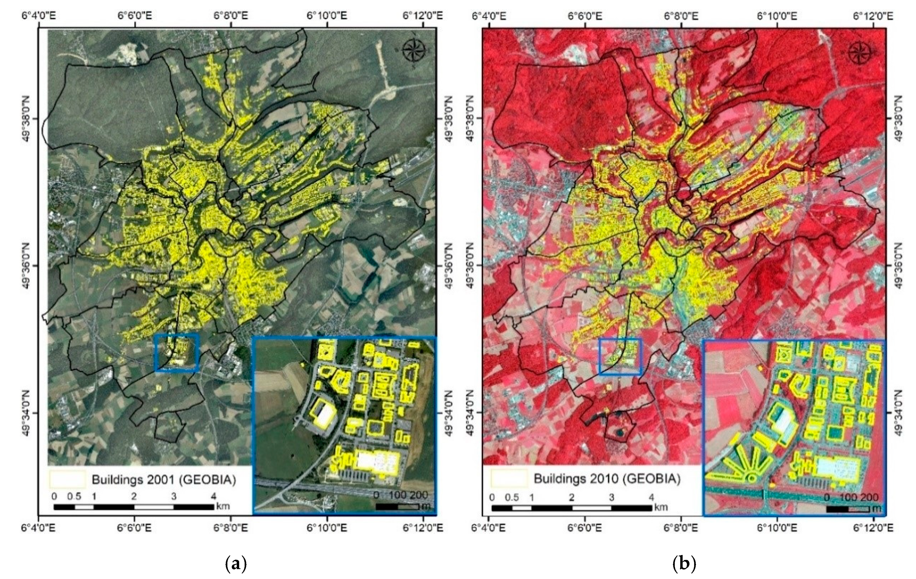
3.1. Buildings Detection and Accuracy Assessment

The results of 3D modeling based on ALS (2019) and object-based classification of CIR (2010) and RGB orthophoto map (2001) are building vector objects that will serve as an input layer for further spatial analysis. The GEOBIA classification results from 2010 show an overall accuracy (OA) of 97.3% with the Kappa index agreement (KIA) of 0.95. The results from 2001 have an OA of 96.0% and Kappa of 0.92. The producer accuracy (PA) and the user accuracy (UA) for buildings and unclassified class are listed in Table 2 and Table 3, based on a randomly selected individual sample reference. The objects representing buildings in 2001 and 2010 were exported to shapefile (Figure 7 and Figure 8).
Based on ALS point cloud acquired in 2019 with a high density about 25 pts/m2, we generated models (LoD2) which include detailed modeling of the shape of roofs (without architectural elements such as skylights, chimneys, antennas, solar panels, etc.) with vertical projection to the ground (Figure 9). The high density of ALS point cloud > 10 pts/m2 allows to generate accurate models with details and roof constructions [51]. At a point cloud density of 25 pts/m2, the XY accuracy of constructed 3D building models was approximately 20 cm. The accuracy of the roof planar surface for the Z coordinate was approximately 10 cm and for the edges 20 cm. The roof shape of the building has been exported to shapefile format and divided into residential and non-residential buildings (Figure 10). A visual assessment of the cadastral shapefile was performed based on orthophoto (2019) to check the correctness of the administrative data.

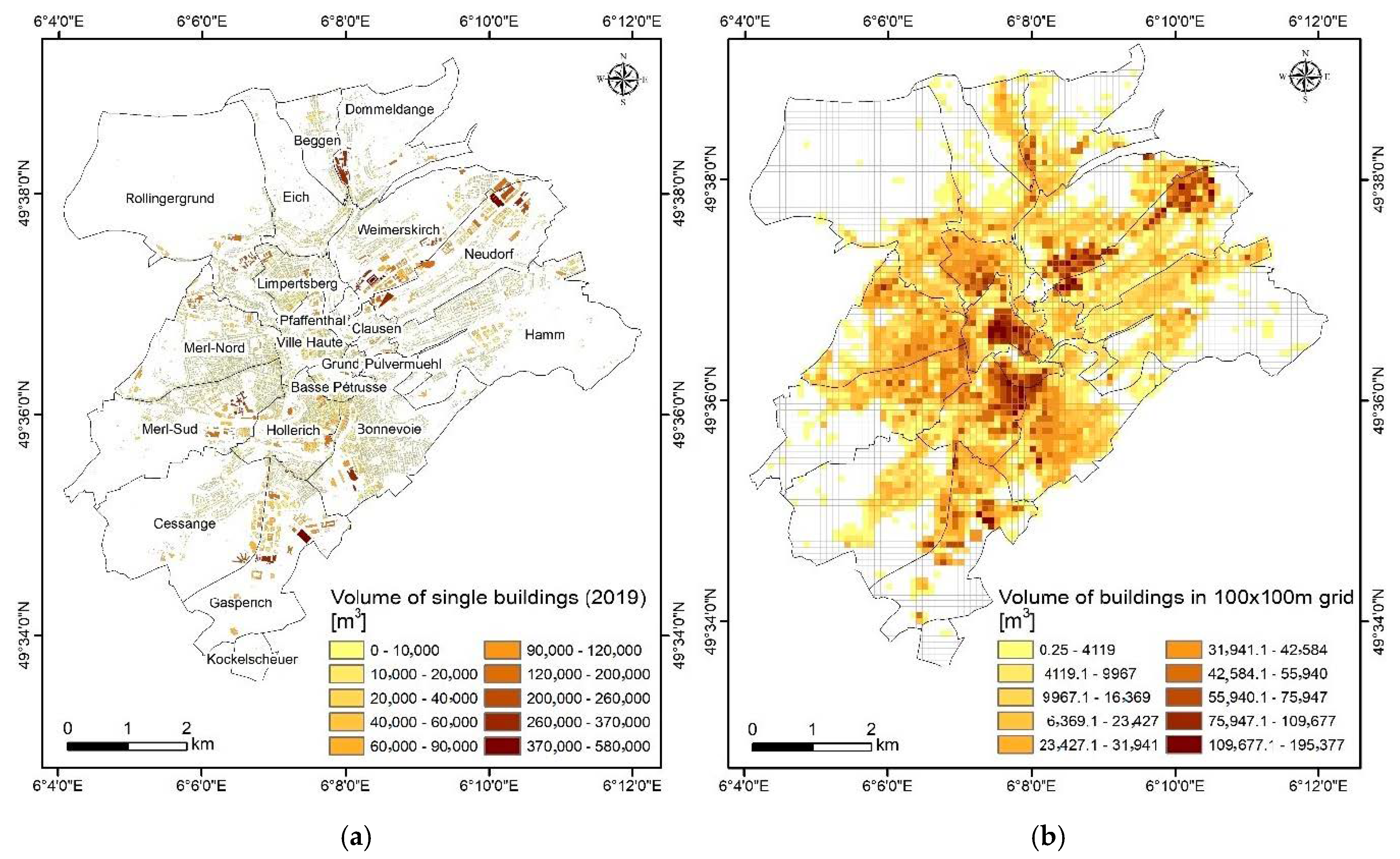
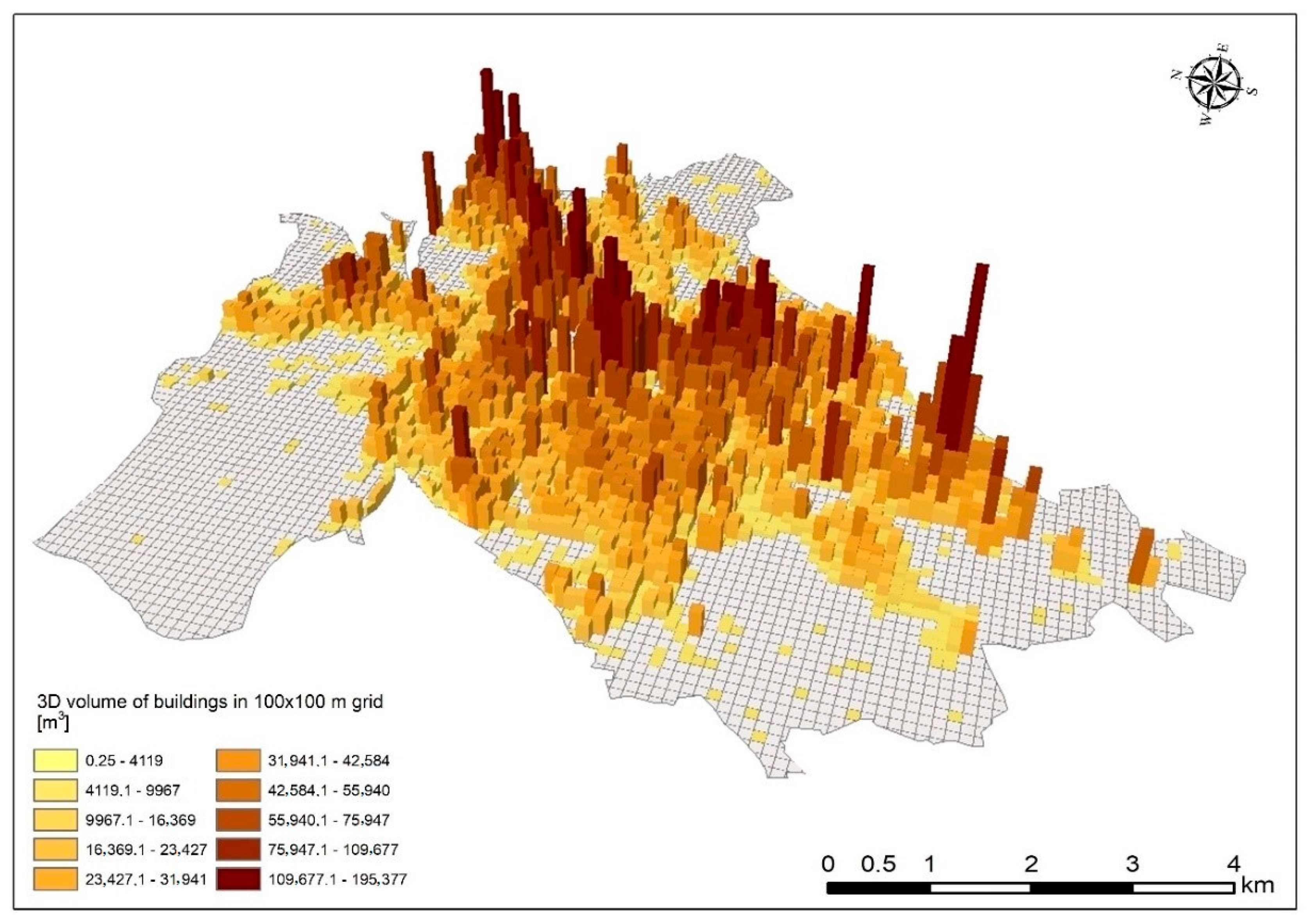
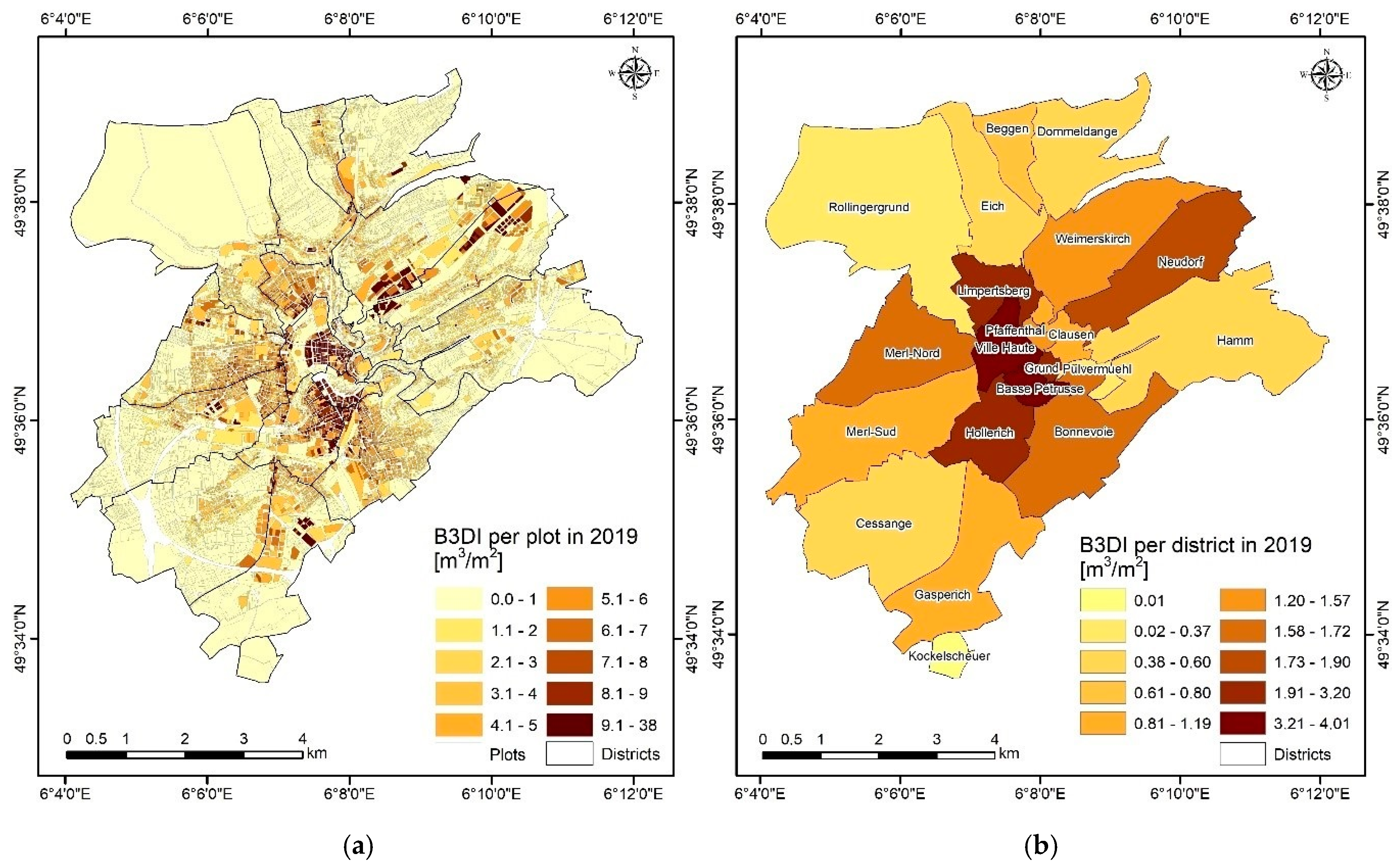
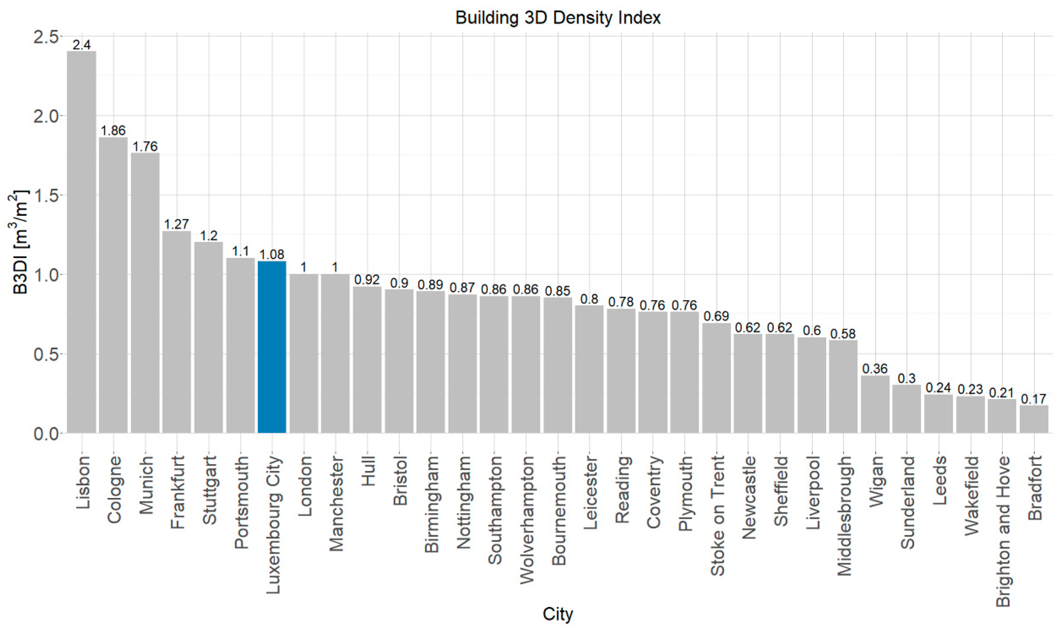
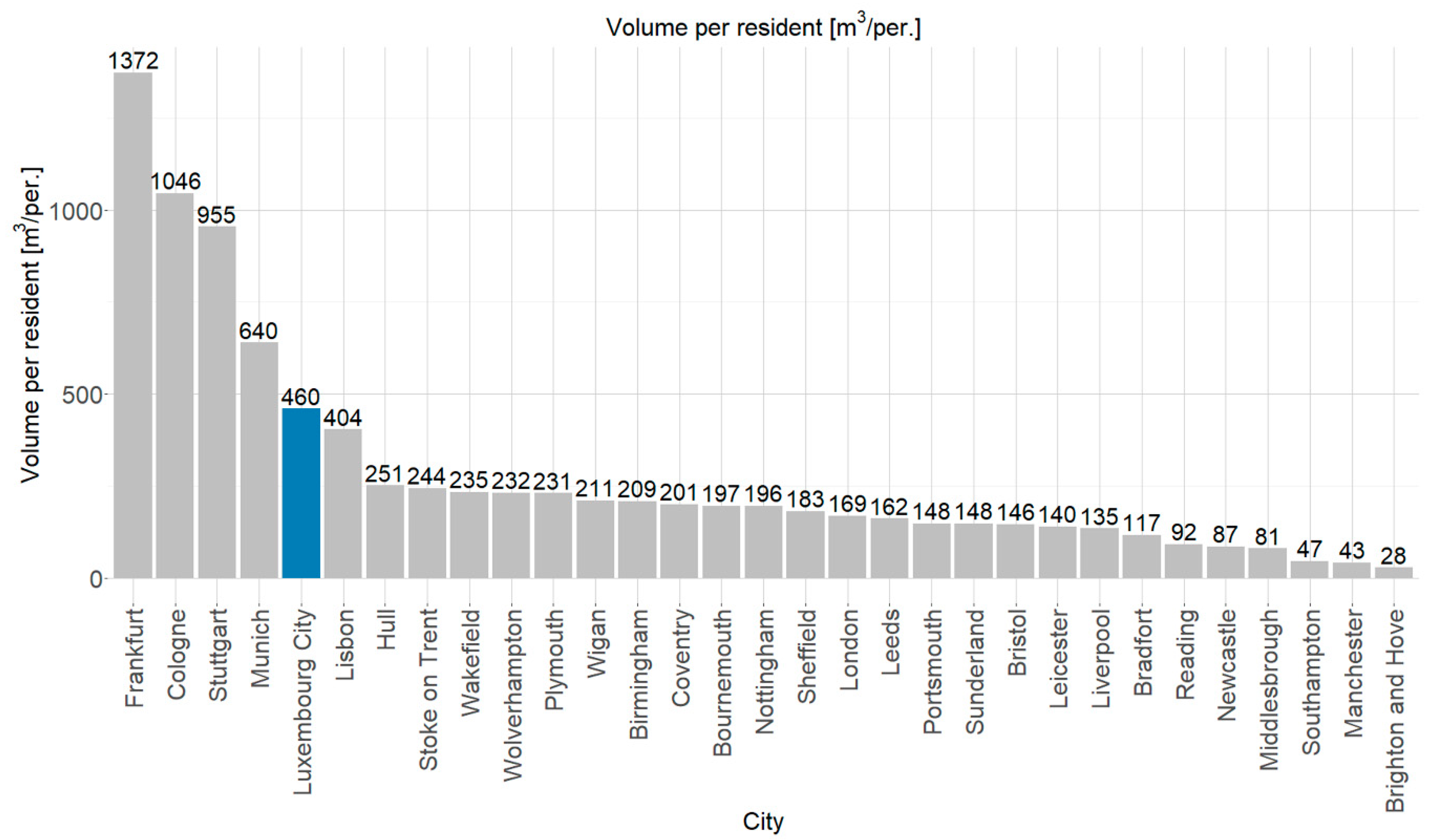
3.2. Urban Volumetry and Building 3D Density Index (B3DI)

The volume calculation and 3D spatial analyses performed on the model of buildings from 2019 show that total building volume in Luxembourg City is about 56 million m3, which is 460 m3 per resident. The mean volume of all types of buildings is 2349 m3 per building. The tallest building (in the business center of Kirchberg) reaches 114 m in height (84,683 m3), and the largest volume of a single building is 580 thousand m3 in Gasperich district (Cloche d’Or Shopping Center). The other largest buildings in the city are hypermarkets in Kirchberg, European Union edifices, some banks, ArcelorMittal company, European School, and hospitals.
The volume in 2019 was calculated separately for the residential and non-residential buildings. The volume of all residential buildings in Luxembourg City is 30 million m3. The mean volume of a residential building is 1460 m3 and the mean height is 12.5 m. Buildings marked as non-residential were assigned to a sub-category: commercial, industrial, or agricultural buildings (86%) and public buildings (14%). The total volume of non-residential buildings is 25 million m3. The mean volume of a non-residential building is about 13 thousand m3 and the mean height is 13.5 m. The volume of individual buildings in the city and in conversion to a 100 × 100 m grid was presented in Figure 11 and Figure 12.
The Building 3D Density Index (B3DI) calculated for the City in 2019 is 1.09 m3/m2. The city center is characterized by the highest B3DI, for the Ville Haute (B3DI > 4.0), Basse Pétrusse and Hollerich district (south of the center) the B3DI > 3.0 (Figure 13). Districts with significantly built-up constitute 57% of all density (B3DI > 1.0). The smallest Building 3D Density Index is found in districts located in the vicinity of the city border: Kockelscheuer, Rollingergrund, Pulvermuehl, Cessange, Eich, Hamm, Dommeldange, and Beggen, with B3DI between 0.01–0.76. A similar distribution occurs for plots of land. The most built-up plots with B3DI > 10.0, that occupy 5.7% of plots in the city are in the center, especially in Ville Haute district and in business parts of Neudorf (Kirchberg), Hollerich, and Gasperich district, where the plots of land are small (mean area of plots is 5.5 are). The level of built-up plots with B3DI between 1.0–10.0 occurs 67.5% of cases, where the average plot size is 670 m2. The plots with the lowest ratio (B3DI < 1.0) are larger plots (mean area is 37 are), which constitute 26.8% and are located mainly outside the city center.
For residential buildings, the total B3DI is 0.59 m3/m2. The residential districts that have the highest indicator value (B3DI > 2.0) are Ville Haute and Limpertsberg (residential area near the center), next Basse Pétrusse, Hollerich, Merl-Nord and Bonnevoie (B3DI > 1.0). Other districts have a low index (B3DI between 0.01–0.89). For non-residential buildings, the total B3DI is 0.49 m3/m2. The highest level of the index falls for the Grund district (B3DI = 1.72), Basse Pétrusse (1.42) in the center of the city, and for the Neudorf district (1.36) with the business part of Kirchberg. The volume of buildings and Building 3D Density Index (B3DI) by districts of Luxembourg City in 2019 is presented in Appendix A (Table A1).
The volume of buildings in 2010 was 46.5 million m3 that is 512.7 m3 per resident in 2010. The total B3DI in 2010 was 0.9 m3/m2, the highest index was in the Ville Haute and Basse Pétrusse district (B3DI > 3.0). Districts that were significantly built-up constituted 48% of all (B3DI > 1.0). The smallest B3DI below 0.5 was in districts: Dommeldange, Hamm, Eich, Cessange, Pulvermuehl, Rollingergrund, and Kockelscheuer. In 2001, the volume of buildings was 40 million m, which is 521.9 m3 per resident. The Building 3D Density Index in 2001 was 0.77 m3/m2. The Ville Haute district had a 3D density index > 3.0, while 43% of the districts showed B3DI > 1. The smallest B3DI was in the same districts as in 2010, and in addition the Gasperich district, which was later significantly developed. Detailed table on the volume of buildings and B3DI in 2001 and 2010 can be found in Appendix A (Table A2).

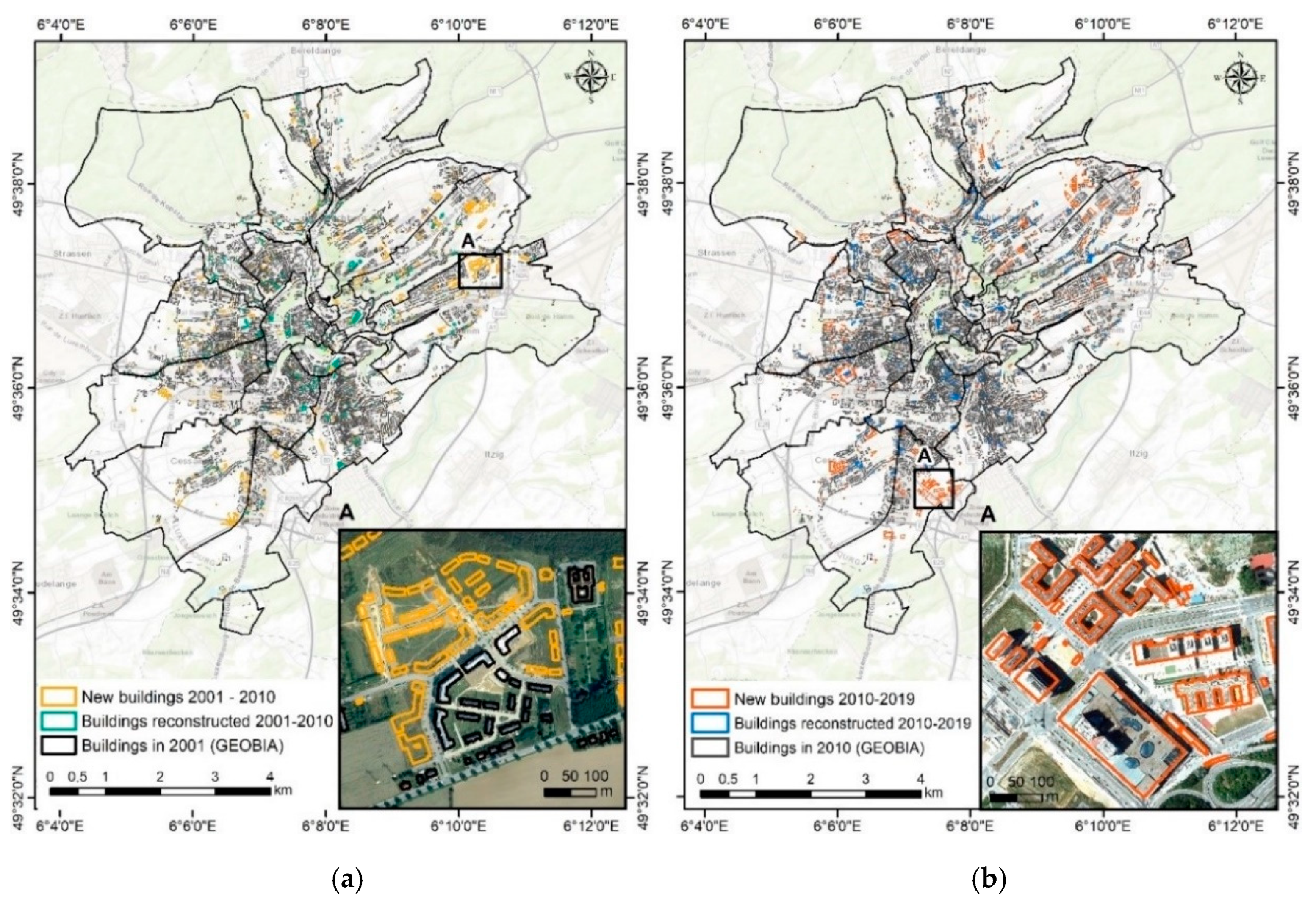
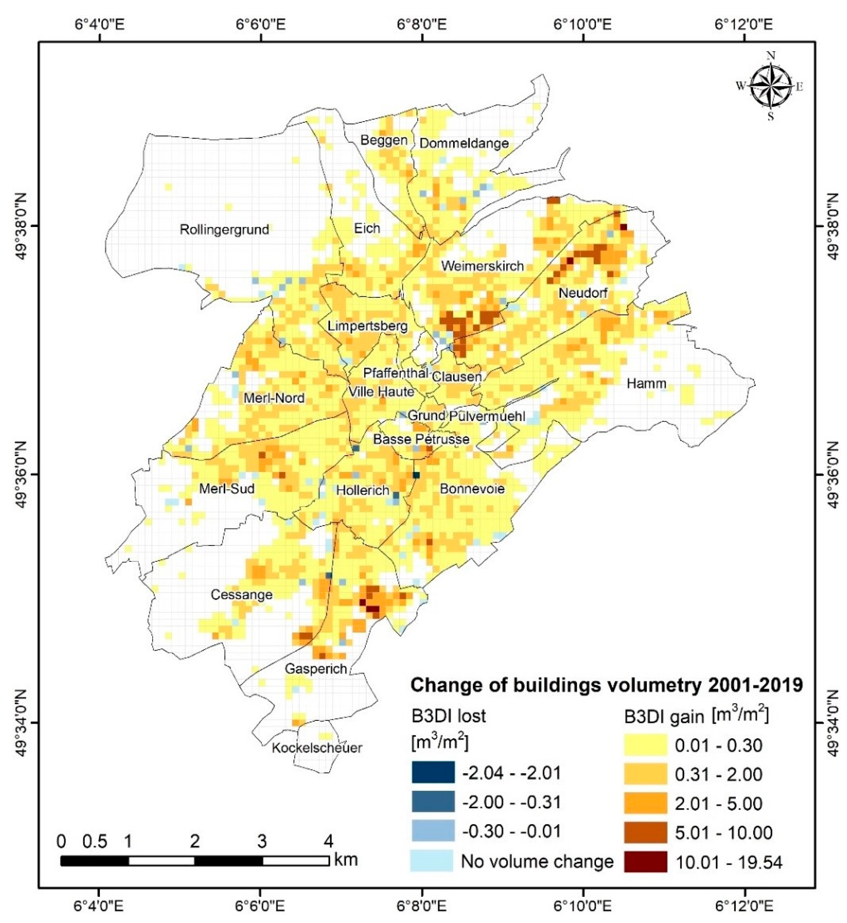
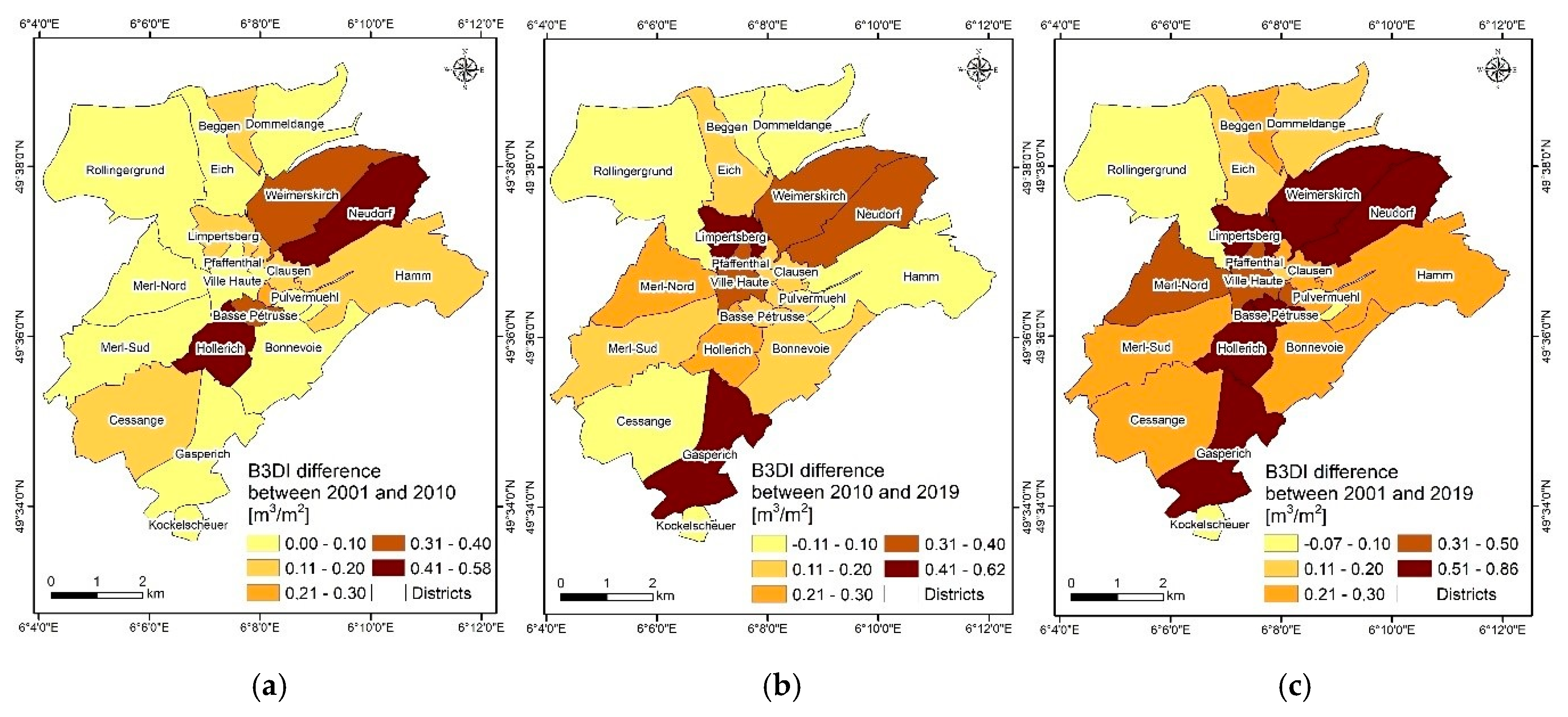
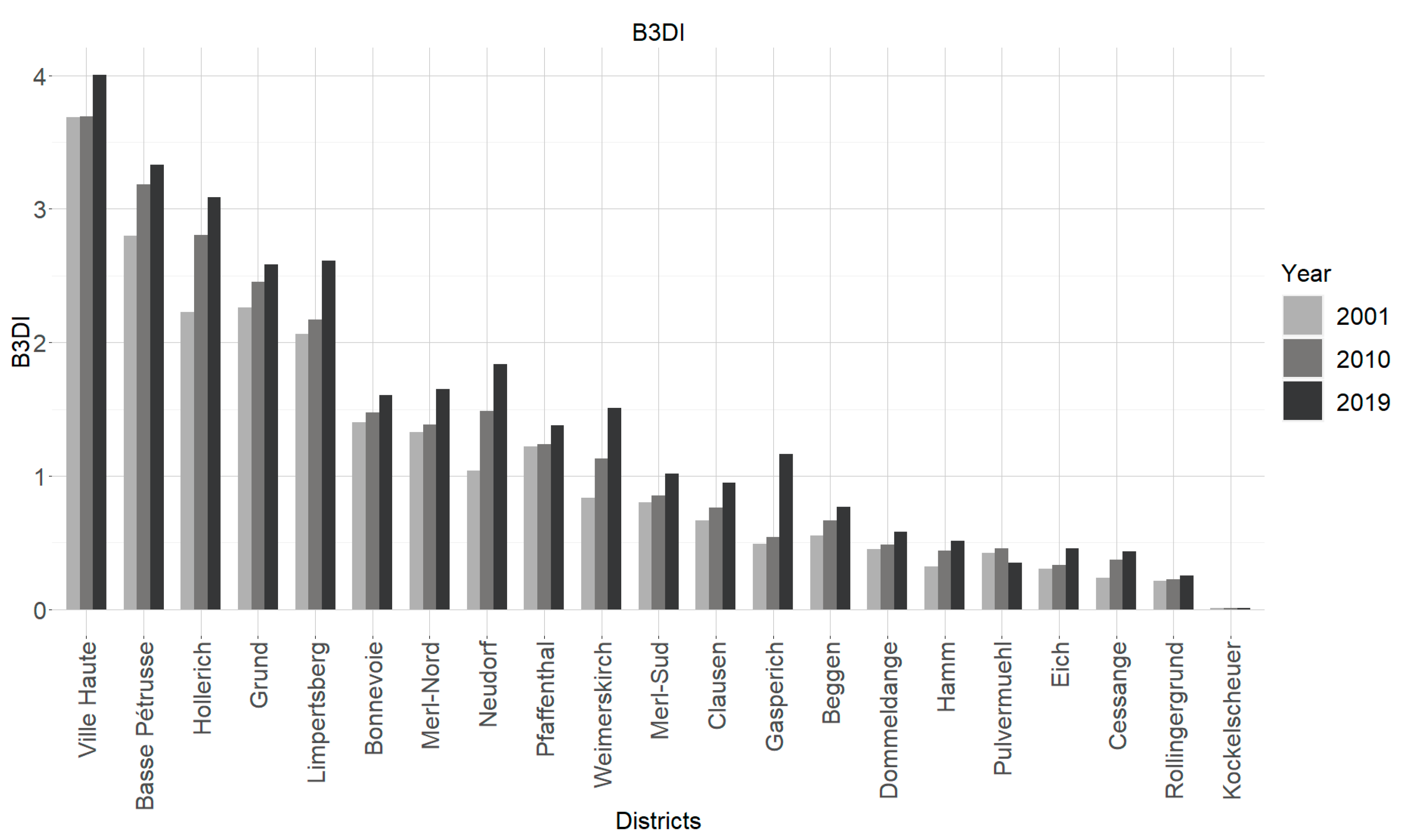
3.3. Changes in City Volumetry over the Past 20 Years

The dynamics of change in building urban volumetry over the last 20 years in Luxembourg City was analyzed by comparing the Building 3D Density Index in grid of 100 m and at the district-level in 2001, 2010, and 2019 (Figure 14 and Figure 15). Overall change in the past 20 years in Buildings 3D Density Index was +0.31 m3/m2, where, between 2001 and 2010, it was +0.13 m3/m2, and between 2010 and 2019 the change was +0.19 m3/m2. Major changes between 2001 and 2010 are observed in the Hollerich (+0.58), Neudorf (+0.45), Basse Pétrusse (+0.39), and Weimerskirch (+0.3) districts. Many new office buildings were built, and the public service part was expanded. At the same time, more than half of the districts have not changed significantly (B3DI change was < 0.1). In the following years (2010 and 2019), the major changes in the districts were observed in Gasperich (+0.62), Limpertsberg (+0.44), Weimerskirch (+0.38), Neudorf (+0.35), and Ville Haute (+0.31) as a result of significant urbanization. In the Pulvermuehl (industrial district) a decrease in the B3DI index (−0.11) was observed, due to the demolition of the factory and new residential and office buildings are planned in the future. Remarkable changes over the last 20 years have occurred in the districts: Hollerich (+0.86), Neudorf (+0.8), Weimerskirch (+0.68), and Gasperich (+0.67) (Figure 16). The Neudorf and Kirchberg districts now enjoy a high level of economic activity. The Kirchberg plateau saw its fields disappear in favor of large buildings with the arrival of the European institutions and still develop financial activities in this district. Weimerskirch is a very attractive residential area. In Gasperich, in 2017 massive construction began on a new development providing for dozens of large office buildings, hundreds of residences and a new shopping center.

4. Discussion

The spatiotemporal monitoring of changes in the volume of built-up areas and 3D modeling of buildings is a very actual topic that can reshape the perception of the urban landscape and the environment in which we live. Our research shows that the combination of up-to-date remote sensing data, spatial data, and archival aerial orthophotos offers an accurate estimation of changes that have occurred in urban volumetry over time and across space. Hence, our methodology allows supplementing incomplete time series data for exploring changes in 3D urban structure using ALS LiDAR point cloud and GEOBIA approach of the archival orthophoto maps. The concepts of the spatial index based on 3D information contained in the ALS point clouds allow for a synthetic representation of the spatial features such as buildings volume and 3D density. The automatic 3D modeling was used to calculate the volume, and by combining the results with data of demolition-reconstruction in plots of land (Housing Observatory project, LISER-Luxembourg), it was possible to use the models in previous years on unmodified buildings, where 3D information was not available. The proposed ruleset of GEOBIA classification yielded high accuracies in 2010 and 2001 with a Kappa respectively of 0.95 (CIR) and 0.92 (RGB).
The 3D spatial indicator developed, concerned the change in building volume density. In the past 20 years, the volume of buildings and B3DI has increased significantly from 0.77 m3/m2 (2001) and 0.9 m3/m2 (2010) to 1.09 m3/m2 (2019). Luxembourg City in 2019 has a volume for all buildings equal to 56 million m3, with an average height of 13 m. The B3DI index of residential buildings has a value of 0.59 m3/m2 and the B3DI index of non-residential buildings has an index of 0.49 m3/m2, which means that the volume of residential buildings still accounts for a larger share at the entire city scale.
The general trend of changes in the volume of buildings per resident shows a decrease from 522 m3/resident in 2001 and513 m3/resident in 2010 to 460 m3/resident in 2019. The most frequently observed situation concerned the demolition of small houses and erecting larger apartments in this place. At the same time, the population increases, and newly built apartments are smaller, but there are more built within a year. In comparison to the continental scale mapping and analysis of 3D building structure with 1 km2 resolution [34], the building volume per resident in Luxembourg City is higher than the average in Europe (404.6 m3) and China (302.3 m3) but it is still lower than in the US (565.4 m3). This value significantly equates to a higher land take and land consumption per person due to the big share of non-residential buildings in the Luxembourg City.
Previous research on 3D cities reported the need to measure similar indicators in many cities. A method with mean height of buildings based on nDSM was used by EMU Analytics to calculate buildings density in 25 cities in United Kingdom, where average of density index indicates 0.68 m3/m2 [36]. Krehl et al. (2016) estimated the built-up volume for the selected cities in Germany, the index was adopted for Cologne, Munich, Frankfurt, and Stuttgart respectively: 1.86 m3/m2, 1.76 m3/m2, 1.27 m3/m2, and 1.20 m3/m2 [37]. Santos et al. (2013) characterized urban volumetry in the city of Lisbon (Portugal) [52]. Built volume was over 204 million m3, which indicates a much higher index (B3DI = 2.4) than in other European cities. The results show that in Luxembourg City the B3DI index and volume of buildings per resident are higher than most of the Cities in the UK and lower than German Cities (Figure 17 and Figure 18). The high value of B3DI for Luxembourg City compared to the UK cities (city borders at municipality level) can be explained by the fact that Luxembourg is a relatively small-sized city (51 km2). However, the separation of residential and non-residential buildings in other European cities is needed for better comparability.
Previous work [53,54], performed the detection of buildings using a similar GEOBIA approach, showed comparable accuracy to our results (KIA: 0.95 and 0.92). Tiwari et al. (2020) developed an object-based algorithm on orthophoto (GSD 0.25 m) to extract all buildings in a small city in Israel with a Kappa index of agreement of 0.95 (UA and PA of the building classes are 99.38% and 98.03%) [53]. Our methodology is not limited to aerial orthophotos, very high resolution (VHR) satellite imagery is often used for building detection and offers high flexibility when it comes to data available. Fan et al. (2016) based on Quickbird-2 image satellites (GSD 0.61 m) extracted information of buildings in an urban area with an overall accuracy of 87% and Kappa value of 0.87 [54]. Warth et al. (2020) predicted socio-economic indicators for urban planning using WorldView-1 (GSD 0.5 m), PlanetScope (3.0 m) satellite imagery, and collected ground-truthing data [55]. The growing number of the upcoming new Earth Observation missions and accompanying increase in VHRS imagery (e.g., Pléiades Neo [56] and WorldView Legion [57]) ensure an average daily revisit time and thus flexibility in terms of available data. Therefore, our approach does not have to depend on the available open data, if we consider the satellite image fee, we can get data from a specific day. Additionally, 3D data is also becoming more common and open access. The wall-to wall LiDAR ALS point clouds coverage is available for many European countries (e.g., in Denmark, Estonia, Finland, Latvia, Luxembourg, the Netherlands, Poland, Slovenia, Spain, Sweden, Switzerland, UK), but time series analysis is still not always possible due to some gaps in the data from several years.
Our study has some limitations. First, lack of ALS LiDAR data for the three years 2001, 2010, and 2019. For this reason, only in 2019, we were able to carry out 3D modeling of buildings. For detecting changes in the last 20 years, we used available data with various resolutions, in 2010 CIR and RGB orthophotos with 0.25 m, and in 2001 only RGB with 0.5 m spatial resolution, but this did not significantly affect the overall accuracy (the difference was 1.3%). To obtain the height of the buildings for the archival data, the Urban Atlas Buildings Height layer (2011) was used to compute the volume of the buildings that had been modified and could cause a significant demolition-restoration error. For buildings that did not change between 2001–2019 and 2010–2019, LiDAR data was used to eliminate errors caused by lower data resolution. The comparison of the results (volume of buildings in 2001, 2010, 2019) obtained by data fusion was possible by using the historical data from the demolition-reconstruction layers, which contained information about buildings that had changed (with details of the date) or buildings which never changed. This allowed the use of LiDAR data wherever no changes were recorded. In 2001, 90.9% of the building volume could be calculated with LiDAR, as no changes were recorded for these buildings between 2001 and 2019. In 2010, as much as 94.5% of the volume of buildings could be calculated with LiDAR, as there was no change between 2010 and 2019 in buildings. Therefore, due to the availability of the demolition-reconstruction layer, the error in comparing the building volumes in 2001, 2010, and 2019 does not affect the results to a large extent. Second, we were unable to assess how index changes for residential buildings because in 2001 and 2010 no cadastral information of this type was available.
Future work will simulate urban densification and assess its socioeconomic, population, environmental impacts, and will monitor urban greenery and its relation to built-up areas. The debate about the urban growth of Luxembourg for the coming future should be open as soon as possible. As the different strategies elaborated 20 years ago concerning polycentric concentration or deconcentrated concentration [58] are not efficient enough and should be revised. Even if the third industrial revolution is coming quickly, it does not resolve all problems of a growing population, urban development, and densification, or big pressure on the land. Luxembourg City is still maintaining its principal role in the country and attracting people to live in the capital. The discussion surrounding the distribution of densities across the urban area can certainly be one of the most controversial issues in urban planning. The measure of the current situation and geovisualization of 3D changes over years assists the analysis of cities and can help urban planners for smart solutions in urban form for future developments. From this perspective, defining volumetric ratios that explain the dynamics of urban areas can bring more clarity to the city’s evolution debate and management of urban space.

5. Conclusions

The methodology presented in is paper that employed ALS LiDAR point cloud and archival aerial orthophotos allows quantifying changes in urban volumetry over time and space. Further, our methodology can provide monitoring based on buildings 3D density index as an effective tool that can be used to characterize the built-up configurations in our cities. Due to the increasingly widespread use of LiDAR technologies, point clouds present valuable spatial information about buildings in a clear and synthetic way, thus being a tool for extracting 3D features difficult to determine by traditional methods. Our findings demonstrate the value of ALS LiDAR data for monitoring effectively the city volume density at some specific dates. Despite airborne laser scanning data is widely recognized as a highly precise data source, time-series data are not available in many cities to detect temporal changes. Therefore, we proposed the use of GEOBIA classification based on archival orthophotos. The ruleset produced for this study to extract buildings can be used in other cities based on CIR aerial photos or VHR satellite images supported by other technology like SLS—satellite laser scanning (e.g., GEDI, ICESat-2 missions NASA) or radar technology (e.g., TerraSAR-X; IceEye-1).
We believe that this paper provides an important methodological approach for urban planners and city authorities. Tracking changes in city volume and 3D index are critical for urban policies that concern equality in the distribution of benefits, e.g., equal access to green spaces and amenities, for city residents. Due to the increasing availability of VHR satellite images and the potential of using unmanned aerial vehicles (UAVs), or the rapidly evolving high-altitude platform station (HAPS) systems for cost-effective mapping of urban areas in 2D/3D, it could ensure constant access to quickly obtain data in an area of interest.

Author Contributions

Conceptualization, H.O., K.S., K.Z.-K., A.M.; Methodology, K.Z.-K., K.S.; Software, K.Z.-K., P.W.; Validation, K.Z.-K., K.S.; Formal Analysis, K.Z.-K., K.S.; Resources, K.S., K.Z.-K.; Data Curation, K.Z.-K., K.S.; Writing—Original Draft Preparation, K.Z.-K., K.S.; Writing—Review & Editing, K.Z.-K., H.O., A.M., P.W., J.T., P.G.; Visualization, K.Z.-K.; Supervision, H.O., J.T., P.G., A.M.; Project Administration, H.O.; Funding Acquisition, H.O. All authors have read and agreed to the published version of the manuscript.

Funding

This research was funded by the INTER program, co-funded by the Fond National de la Recherche, Luxembourg (FNR) and the Fund for Scientific Research-FNRS, Belgium (F.R.S—FNRS), grant number 19-14016367—“Sustainable Residential Densification” project (SusDens, 2020–2023).

Acknowledgments

We thank the Housing Observatory, a collaboration between the Luxembourg Housing Ministry and the Luxembourg Institute for Socio-Economic Research, for providing access to their data.

Conflicts of Interest

The authors declare no conflict of interest.

Appendix A

Table A1. Volume of buildings and Building 3D Density Index (B3DI) for residential (R) and non-residential (NR) buildings in Luxembourg City in 2019.
DistrictsAreaVolume
All
B3DI
All
Volume
R
B3DI
R
Volume
NR
B3DI
NR
Name[m2][m3][m3/m2][m3][m3/m2][m3][m3/m2]
Ville Haute1,058,465.544,241,563.934.012,965,917.062.801,275,646.871.21
Basse Pétruss453,111.051,508,814.683.33863,309.871.91645,504.811.42
Hollerich1,800,838.975,560,073.123.093,232,718.751.802,327,354.371.29
Limpertsberg1,176,055.913,073,585.622.612,356,861.752.00716,723.870.61
Grund155,076.80400,620.122.58134,047.560.86266,572.561.72
Neudorf3,220,259.145,923,257.371.841,542,721.430.484,380,535.941.36
Merl-Nord2,890,428.024,767,710.431.653,299,263.371.141,468,447.060.51
Bonnevoie3,546,872.295,697,965.931.613,823,082.431.081,874,883.500.53
Weimerskirch3,522,342.375,323,061.251.511,680,753.500.483,642,307.751.03
Pfaffenthal175,462.57242,085.751.38156,145.560.8985,940.190.49
Gasperich3,449,516.404,006,822.431.16635,693.430.183,371,129.000.98
Merl-Sud4,011,460.834,069,067.811.012,743,936.250.681,325,131.560.33
Clausen601,469.02571,229.930.95249,419.430.41321,810.500.54
Beggen1,133,763.20867,089.810.76718,394.620.63148,695.190.13
Dommeldange2,926,149.861,693,941.060.58650,902.870.221,043,038.190.36
Hamm5,775,969.442,974,906.930.522,233,381.430.39741,525.500.13
Eich2,381,337.221,090,239.430.46853,657.810.36236,581.620.10
Cessange4,934,991.402,149,884.180.441,154,016.310.23995,867.870.20
Pulvermuehl302,362.01105,390.060.3575,326.250.2530,063.810.10
Rollingergrund7,790,154.861,974,078.500.251,280,569.560.16693,508.940.09
Kockelscheuer428,491.163732.250.013720.180.0112.070.00
Luxembourg City51,734,578.0656,245,120.591.0930,653,839.420.5925,591,281.170.49
Table A2. Volume of buildings and Building 3D Density Index (B3DI) in Luxembourg City in 2001 and 2010.
DistrictsAreaVolume Buildings 2001B3DI 2001Volume Buildings 2010B3DI 2010
Name[m2][m3][m3/m2][m3][m3/m2]
Ville Haute1,058,465.543,900,303.133.683,910,583.683.69
Basse Pétrusse453,111.051,267,927.252.801,443,160.433.19
Hollerich1,800,838.974,012,451.862.235,054,810.872.81
Limpertsberg1,176,055.912,425,831.812.062,553,438.432.17
Grund155,076.80350,627.132.26380,842.432.46
Neudorf3,220,259.143,340,875.631.044,780,859.811.48
Merl-Nord2,890,428.023,831,744.441.334,007,072.431.39
Bonnevoie3,546,872.294,961,248.691.405,236,639.311.48
Weimerskirch3,522,342.372,937,256.440.833,982,745.51.13
Pfaffenthal175,462.57214,528.8751.22217,273.931.24
Gasperich3,449,516.401,694,743.560.491,856,934.370.54
Merl-Sud4,011,460.833,210,661.380.803,423,023.680.85
Clausen601,469.02399,212.130.66459,198.930.76
Beggen1,133,763.20626,895.060.55755,686.250.67
Dommeldange2,926,149.861,323,0580.451,420,293.180.49
Hamm5,775,969.441,849,161.060.322,550,945.120.44
Eich2,381,337.22722,590.130.30791,180.930.33
Cessange4,934,991.401,159,6930.231,820,0100.37
Pulvermuehl302,362.01126,9430.42138,498.810.46
Rollingergrund7,790,154.861,668,265.250.211,765,808.250.23
Kockelscheuer428,491.163567.50.013597.250.01
Luxembourg City51,734,578.0640,027,585.300.7746,552,603.590.90

References

  1. Anees, M.M.; Mann, D.; Sharma, M.; Banzhaf, E.; Joshi, P.K. Assessment of Urban Dynamics to Understand Spatiotemporal Differentiation at Various Scales Using Remote Sensing and Geospatial Tools. Remote Sens. 2020, 12, 1306. [Google Scholar] [CrossRef] [Green Version]
  2. Kajimoto, M.; Susaki, J. Urban Density Estimation from Polarimetric SAR Images Based on a POA Correction Method. IEEE J. Sel. Top. Appl. Earth Obs. Remote Sens. 2013, 6, 1418–1429. [Google Scholar] [CrossRef] [Green Version]
  3. Peng, F.; Gong, J.; Wang, L.; Wu, H.; Yang, J. Impact of building heights on 3D urban density estimation from spaceborne stereo imagery. Int. Arch. Photogramm. Remote Sens. Spat. Inf. Sci. 2016, 41, 677–683. [Google Scholar] [CrossRef]
  4. Gonzalez-Aguilera, D.; Crespo-Matellan, E.; Hernandez-Lopez, D.; Rodriguez-Gonzalvez, P. Automated Urban Analysis Based on LiDAR-Derived Building Models. IEEE Trans. Geosci. Remote Sens. 2013, 51, 1844–1851. [Google Scholar] [CrossRef]
  5. Zhang, T.; Huang, X.; Wen, D.; Li, J. Urban Building Density Estimation from High-Resolution Imagery Using Multiple Features and Support Vector Regression. IEEE J. Sel. Top. Appl. Earth Obs. Remote Sens. 2017, 10, 3265–3280. [Google Scholar] [CrossRef]
  6. Yu, B.; Liu, H.; Wu, J.; Hu, Y.; Zhang, L. Automated derivation of urban building density information using airborne LiDAR data and object-based method. Landsc. Urban Plan. 2010, 98, 210–219. [Google Scholar] [CrossRef]
  7. Unsalan, C.; Boyer, K.L. A system to detect houses and residential street networks in multispectral satellite images. Comput. Vis. Image Underst. 2005, 98, 423–461. [Google Scholar] [CrossRef]
  8. Thiele, A.; Cadario, E.; Schulz, K.; Thonnessen, U.; Soergel, U. Building recognition from multi-aspect high-resolution InSAR data in urban areas. IEEE Trans. Geosci. Remote Sens. 2007, 45, 3583–3593. [Google Scholar] [CrossRef]
  9. San, D.K.; Turker, M. Building extraction from high resolution satellite images using hough transform. Int. Arch. Photogramm. Remote Sens. Spat. Inf. Sci. 2010, 38, 1063–1068. [Google Scholar]
  10. Wang, L.; Omrani, H.; Zhao, Z.; Francomano, D.; Li, K.; Pijanowski, B. Analysis on urban densification dynamics and future modes in southeastern Wisconsin, USA. PLoS ONE 2019, 14, e0211964. [Google Scholar] [CrossRef]
  11. Pili, S.; Grigoriadis, E.; Carlucci, M.; Clemente, M.; Salvati, L. Towards sustainable growth? A multi-criteria assessment of (changing) urban forms. Ecol. Indic. 2017, 76, 71–80. [Google Scholar] [CrossRef]
  12. Aburas, M.M.; Ho, Y.M.; Ramli, M.F.; Ash’aari, Z.H. Monitoring and assessment of urban growth patterns using spatio-temporal built-up area analysis. Environ. Monit. Assess. 2018, 190, 156. [Google Scholar] [CrossRef] [PubMed]
  13. Blaschke, T.; Hay, G.J.; Kelly, M.; Lang, S.; Hofmann, P.; Addink, E.; Tiede, D. Geographic object based image analysis—Towards a new paradigm. Isprs J. Photogramm. Remote Sens. 2014, 87, 180–191. [Google Scholar] [CrossRef] [Green Version]
  14. Benz, U.C.; Hofmann, P.; Willhauck, G.; Lingenfelder, I.; Heynen, M. Multi-resolution, object-oriented fuzzy analysis of remote sensing data for GIS-ready information. ISPRS J. Photogramm. Remote Sens. 2004, 58, 239–258. [Google Scholar] [CrossRef]
  15. Chen, G.; Weng, Q.; Hay, G.J.; He, Y. Geographic object-based image analysis (GEOBIA): Emerging trends and future opportunities. GISci. Remote Sens. 2018, 55, 159–182. [Google Scholar] [CrossRef]
  16. Wężyk, P.; Hawryło, P.; Szostak, M. Determination of the number of trees in the Bory Tucholskie National Park using crown delineation of the canopy height models derived from aerial photos matching and airborne laser scanning data. Arch. Fotogram. Kartogr. Teledetekcji 2016, 28, 137–156. [Google Scholar] [CrossRef]
  17. Simonetto, E.; Oriot, H.; Garello, R. Rectangular building extraction from stereoscopic airborne radar images. IEEE Trans. Geosci. Remote Sens. 2005, 43, 2386–2395. [Google Scholar] [CrossRef]
  18. Sohn, G.; Dowman, I. Data fusion of high-resolution satellite imagery and LiDAR data for automatic building extraction. ISPRS J. Photogramm. Remote Sens. 2007, 62, 43–63. [Google Scholar] [CrossRef]
  19. Turlapaty, A.; Gokaraju, B.; Du, Q.; Younan, N.H.; Aanstoos, J.V. A hybrid approach for building extraction from spaceborne multi-angular optical imagery. IEEE J. Sel. Top. Appl. Earth Obs. Remote Sens. 2012, 5, 89–100. [Google Scholar] [CrossRef]
  20. Davydova, K.; Cui, S.; Reinartz, P. Building footprint extraction from digital surface models using neural networks. In Proceedings of the Image and Signal Processing for Remote Sensing XXII, Edinburgh, UK, 26–28 September 2016; Volume 1004, p. 100040J. [Google Scholar] [CrossRef] [Green Version]
  21. Bittner, K.; Adam, F.; Cui, S.; Korner, M.; Reinartz, P. Building footprint extraction from VHR remote sensing images combined with normalized DSMs using fused fully convolutional networks. IEEE J. Sel. Top. Appl. Earth Obs. Remote Sens. 2018, 11, 2615–2629. [Google Scholar] [CrossRef] [Green Version]
  22. Zhu, Z.; Zhou, Y.; Seto, K.C.; Stokes, E.C.; Deng, C.; Pickett, S.T.A.; Taubenböck, H. Understanding an urbanizing planet: Strategic directions for remote sensing. Remote Sens. Environ. 2019, 228, 164–182. [Google Scholar] [CrossRef]
  23. Shao, Y.; Taff, G.N.; Walsh, S.J. Shadow detection and building-height estimation using IKONOS data. Int. J. Remote Sens. 2011, 32, 6929–6944. [Google Scholar] [CrossRef]
  24. Kadhim, N.; Mourshed, M. A shadow-overlapping algorithm for estimating building heights from VHR satellite images. IEEE Geosci. Remote Sens. Lett. 2018, 15, 8–12. [Google Scholar] [CrossRef] [Green Version]
  25. Brunner, D.; Lemoine, G.; Bruzzone, L.; Greidanus, H. Building height retrieval from VHR SAR imagery based on an iterative simulation and matching technique. IEEE Trans. Geosci. Remote Sens. 2010, 48, 1487–1504. [Google Scholar] [CrossRef]
  26. Wang, Z.; Jiang, L.; Lin, L.; Yu, W. Building height estimation from high resolution SAR imagery via model-based geometrical structure prediction. Prog. Electromagn. Res. 2015, 41, 11–24. [Google Scholar] [CrossRef] [Green Version]
  27. Sun, Y.; Hua, Y.; Mou, L.; Zhu, X.X. Large-scale building height estimation from single VHR SAR image using fully convolutional network and GIS building footprints. Joint Urb. Remote Sens. Event JURSE 2019, 90, 1–4. [Google Scholar]
  28. Aguilar, M.A.; Saldana, M.; Aguilar, F.J. Generation and quality assessment of stereo-extracted DSM from GeoEye-1 and WorldView-2 imagery. IEEE Trans. Geosci. Remote Sens. 2014, 52, 1259–1271. [Google Scholar] [CrossRef]
  29. Zeng, C. Automated Building Information Extraction and Evaluation from High-Resolution Remotely Sensed Data. Electron. Thesis Diss. Repos. 2014, 2076. Available online: https://ir.lib.uwo.ca/etd/2076 (accessed on 11 October 2020).
  30. Lillesand, T.M.; Kiefer, R.W.; Chipman, J. Lidar Data Analysis and Applications. In Remote Sensing and Image Interpretation, 7th ed.; John Wiley & Sons: Hoboken, NJ, USA, 2015; pp. 475–482. [Google Scholar]
  31. Kedron, P.; Zhao, Y.; Frazier, A.E. Three dimensional (3D) spatial metrics for objects. Landsc. Ecol. 2019, 34, 2123–2132. [Google Scholar] [CrossRef]
  32. Park, Y.; Guldmann, J.M. Creating 3D city models with building footprints and LiDAR point cloud classification: A machine learning approach. Comput. Environ. Urban Syst. 2019, 75, 76–89. [Google Scholar] [CrossRef]
  33. Toschi, I.; Nocerino, E.; Remondino, F. Geomatics makes smart cities a reality. GIM Int. 2017, 31, 25–27. [Google Scholar]
  34. Li, M.; Koks, E.; Taubenböc, H.; Vliet, J. Continental-scale mapping and analysis of 3D building structure. Remote Sens. Environ. 2020, 245, 111859. [Google Scholar] [CrossRef]
  35. Wang, P.; Huang, C.; Tilton, J. Mapping Three-dimensional Urban Structure by Fusing Landsat and Global Elevation Data. arXiv 2018, arXiv:1807.04368. [Google Scholar]
  36. EMU Analytics. Available online: https://buildingheights.emu-analytics.net (accessed on 10 March 2020).
  37. Krehl, A.; Siedentop, S.; Taubenböck, H.; Wurm, M. A comprehensive view on urban spatial structure: Urban density patterns of German City Regions. ISPRS Int. J. Geo Inf. 2016, 5, 76. [Google Scholar] [CrossRef] [Green Version]
  38. Shirowzhan, S.; Trinder, J.; Osmond, P. New Metrics for Spatial and Temporal 3D Urban Form Sustainability Assessment Using Time Series Lidar Point Clouds and Advanced GIS Techniques. Intechopen [Online First] 2019. Available online: https://www.intechopen.com/online-first/new-metrics-for-spatial-and-temporal-3d-urban-form-sustainability-assessment-using-time-series-lidar (accessed on 11 October 2020).
  39. Decoville, A.; Schneider, M. Can the 2050 zero land take objective of the EU be reliably monitored? A comparative study. J. Land Use Sci. 2016, 11, 331–349. [Google Scholar] [CrossRef]
  40. STATEC. Atlas Démographique du Luxembourg; STATEC Institut National de la Statistique et des Études Économiques: Luxembourg, 2019; Volume 2.
  41. Omrani, H.; Abdallah, F.; Charif, O.; Longford, N.T. Multi-label class assignment in land-use modelling. Int. J. Geogr. Inf. Sci. 2015, 29, 1023–1041. [Google Scholar] [CrossRef]
  42. Omrani, H.; Tayyebi, A.; Pijanowski, B. Integrating the multi-label land-use concept and cellular automata with the artificial neural network-based Land Transformation Model: An integrated ML-CA-LTM modeling framework. Gisc. Remote Sens. 2017, 54, 283–304. [Google Scholar] [CrossRef] [Green Version]
  43. Housing Observatory. 2013. Available online: http://observatoire.liser.lu/pdfs/DossierThematique_OBS_2013.pdf (accessed on 30 May 2020).
  44. Housing Observatory. 2019. Available online: http://observatoire.liser.lu/pdfs/DossierThematique_OBS_2019_02.pdf (accessed on 30 May 2020).
  45. Baatz, M.; Schape, A. Multiresolution segmentation: An optimization approach for high quality multi-scale image segmentation. J. Photogramm. Remote Sens. 2000, 58, 12–23. [Google Scholar]
  46. Zięba-Kulawik, K.; Wężyk, P. Detekcja zmian roślinności wysokiej Krakowa w latach 2016–2017 przy wykorzystaniu analizy GEOBIA zobrazowań satelitarnych RapidEye (Planet). Współczesne Probl. Kierun. Badaw. Geogr. Inst. Geogr. Gospod. Przestrz. UJ 2019, 7, 199–226. [Google Scholar]
  47. Wężyk, P.; Hawryło, P.; Janus, B.; Weidenbach, M.; Szostak, M. Forest cover changes in Gorce NP (Poland) using photointerpretation of analogue photographs and GEOBIA of orthophotos and nDSM based on image-matching based approach. Eur. J. Remote Sens. 2018, 51, 501–510. [Google Scholar] [CrossRef]
  48. Congalton, R.G.; Green, K. Assessing the Accuracy of Remotely Sensed Data Principles and Practices, 2nd ed.; CRC Press Taylor & Francis Group: Boca Raton, FL, USA, 2009. [Google Scholar]
  49. Foody, G.M. Status of land cover classification accuracy assessment. Remote Sens. Environ. 2002, 80, 185–201. [Google Scholar] [CrossRef]
  50. Chen, X.; Yu, Y.; Zhu, P. Study from Building Density to Building 3D Density. In Proceedings of the IEEE International Conference on Management and Service Science, Wuhan, China, 20–22 September 2009; pp. 1–5. [Google Scholar] [CrossRef]
  51. TerraScan User’s Guide. 2016. Available online: https://www.terrasolid.com/download/tscan.pdf (accessed on 12 March 2020).
  52. Santos, T.; Rodrigues, A.M.; Tenedório, J.A. Characterizing urban volumetry using LiDAR data. Int. Arch. Photogramm. Remote Sens. Spat. Inf. Sci. 2013, 40, 71–75. [Google Scholar] [CrossRef] [Green Version]
  53. Tiwari, A.; Meir, I.A.; Karnieli, A. Object-based image procedures for assessing the solar energy photovoltaic potential of heterogeneous rooftops using airborne LiDAR and orthophoto. Remote Sens. 2020, 12, 223. [Google Scholar] [CrossRef] [Green Version]
  54. Fan, S.; Liu, Z.; Hu, Y. Extraction of Building Information Using Geographic Object-Based Image Analysis. In Proceedings of the 4th International Workshop on Earth Observation and Remote Sensing Applications (EORSA), Guangzhou, China, 4–6 July 2016. [Google Scholar] [CrossRef]
  55. Warth, G.; Braun, A.; Assmann, O.; Fleckenstein, K.; Hochschild, V. Prediction of socio-economic indicators for urban planning using VHR satellite imagery and spatial analysis. Remote Sens. 2020, 12, 1730. [Google Scholar] [CrossRef]
  56. Airbus Defence and Space. Pléiades Neo. Trusted Intelligence. Available online: https://www.intelligence-airbusds.com/en/8671-pleiades-neo-trusted-intelligence (accessed on 31 July 2020).
  57. Maxar. WorldView Legion. Our Next-Generation Constellation. Available online: https://www.maxar.com/splash/worldview-legion (accessed on 31 July 2020).
  58. Programme Directeur d’Amenagement du Territoire. 2003. Available online: https://amenagement-territoire.public.lu/damassets/fr/publications/documents/programme_directeur/programme_directeur_2003_fr_partie_a_hr.pdf (accessed on 15 May 2020).
Figure 1. (a) Location of the study area. Left top: location of Luxembourg in Europe, left bottom: Grand Duchy of Luxembourg and Luxembourg City borders; (b) Orthophotomap of Luxembourg City at municipality level (2019).
Remotesensing 12 03668 g001
Figure 2. Workflow of the performed analyses (ALS—airborne laser scanning; nDSM—normalized digital surface model; LoD2—level of details 2; GEOBIA—geographic object-based image analysis; B3DI—Building 3D Density Index).
Remotesensing 12 03668 g002
Figure 3. nDSM of building, vegetation and cranes on newly constructed buildings (a); nDSM of buildings only (b).
Remotesensing 12 03668 g003
Figure 4. Classified ALS point cloud (2019); class (2) ground in pink color; class (6) buildings—in red; and vegetation—in green color.
Remotesensing 12 03668 g004
Figure 5. Stages of the GEOBIA building segmentation and classification in eCognition software (Trimble Geospatial); 1—input data: CIR orthophoto; 2—multiresolution segmentation; 3—spectral difference segmentation; 4—classification: buildings class.
Remotesensing 12 03668 g005
Figure 6. Flowchart of the GEOBIA classification process.
Remotesensing 12 03668 g006
Figure 7. GEOBIA classification of buildings based on (a) RGB aerial orthophoto maps in 2001 and (b) CIR orthophoto maps in 2010.
Remotesensing 12 03668 g007
Figure 8. New and reconstructed buildings between (a) 2001–2010 and (b) 2010–2019 in Luxembourg City.
Remotesensing 12 03668 g008
Figure 9. A 3D model (LoD2) of the buildings in Luxembourg City based on ALS point cloud (2019); (a) business district at the northeast (Kirchberg) with public buildings; (b) southern part of the city near the central station.
Remotesensing 12 03668 g009
Figure 10. Residential and non-residential buildings based on ALS point cloud (2019) and cadastral data in Luxembourg City (a); (b) Ville Haute as a residential district (at the right top, b-1), and Gasperich a non-residential part (at the right bottom, b-2).
Remotesensing 12 03668 g010
Figure 11. Luxembourg City maps (2019) of (a) single buildings volume and (b) rasterized map (100 m GSD).
Remotesensing 12 03668 g011
Figure 12. Volume of buildings in a grid (100 × 100 m) in 3D view (Luxembourg City, 2019).
Remotesensing 12 03668 g012
Figure 13. Building 3D Density Index per plot (a) and per district in Luxembourg City in 2019 (b).
Remotesensing 12 03668 g013
Figure 14. Change of buildings volumetry between 2001 and 2019 in Luxembourg City in a grid (100 × 100 m).
Remotesensing 12 03668 g014
Figure 15. Changes of the B3DI index in Luxembourg City districts over the last 20 years; differences between 2001–2010 (a); 2010–2019 (b); between 2001–2019 (c).
Remotesensing 12 03668 g015
Figure 16. The B3DI value of Luxembourg City districts of in years 2001, 2010, and 2019.
Remotesensing 12 03668 g016
Figure 17. Buildings 3D Density Index in European cities (Source: based on data in publication [44,45,54]).
Remotesensing 12 03668 g017
Figure 18. Volume of buildings per resident in European cities (Source: based on data in publication [44,45,54]).
Remotesensing 12 03668 g018
Table 1. Details of geospatial data used in the study.
Data NameData SourcesDate of Data AcqusitionFormatDensity/GSD/Resolution/Accuracy
ALS LiDAR point cloudOpen Data 17–25 February 2019.las~15 pts/m2
Orthophotos RGB/CIROpen Data 124–26 August 2001 3.tif0.50 m
1–2 July 20100.25 m
22 August 20190.20 m
Cadastral shapefileOpen Data 124 February 2019.shp-
Demolition-reconstruction informationHousing Observatory 2 2001–2019.shp-
Urban Atlas—Building HeightEuropean Environment Agency2011.tif10 m
Corine Land Cover (CLC)European Environment Agency2000.shp25 m
201225 m
201810 m
1data.public.lu/en/datasets/; 2 Luxembourg Housing Ministry and the LISER; 3 CIR was not available.
Table 2. Error matrix for the GEOBIA analysis in 2001 (PA: producer accuracy; UA: user accuracy).
Classification Results/Reference DataBuildingsUnclassifiedSumUA (%)
Buildings142714995.3
Unclassified514414996.6
Sum147151
PA (%)96.695.4
Overall Accuracy96.0%
Table 3. Error matrix for the GEOBIA analysis in 2010.
Classification Results/Reference DataBuildingsUnclassifiedSumUA (%)
Buildings144514996.6
Unclassified314614998.0
Sum147151
PA (%)98.096.7
Overall Accuracy97.3%
Publisher’s Note: MDPI stays neutral with regard to jurisdictional claims in published maps and institutional affiliations.

