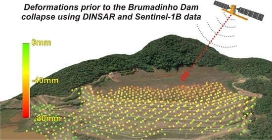
Deformations Prior to the Brumadinho Dam Collapse Revealed by Sentinel-1 InSAR Data Using SBAS and PSI Techniques


Abstract
:
1. Introduction and Context
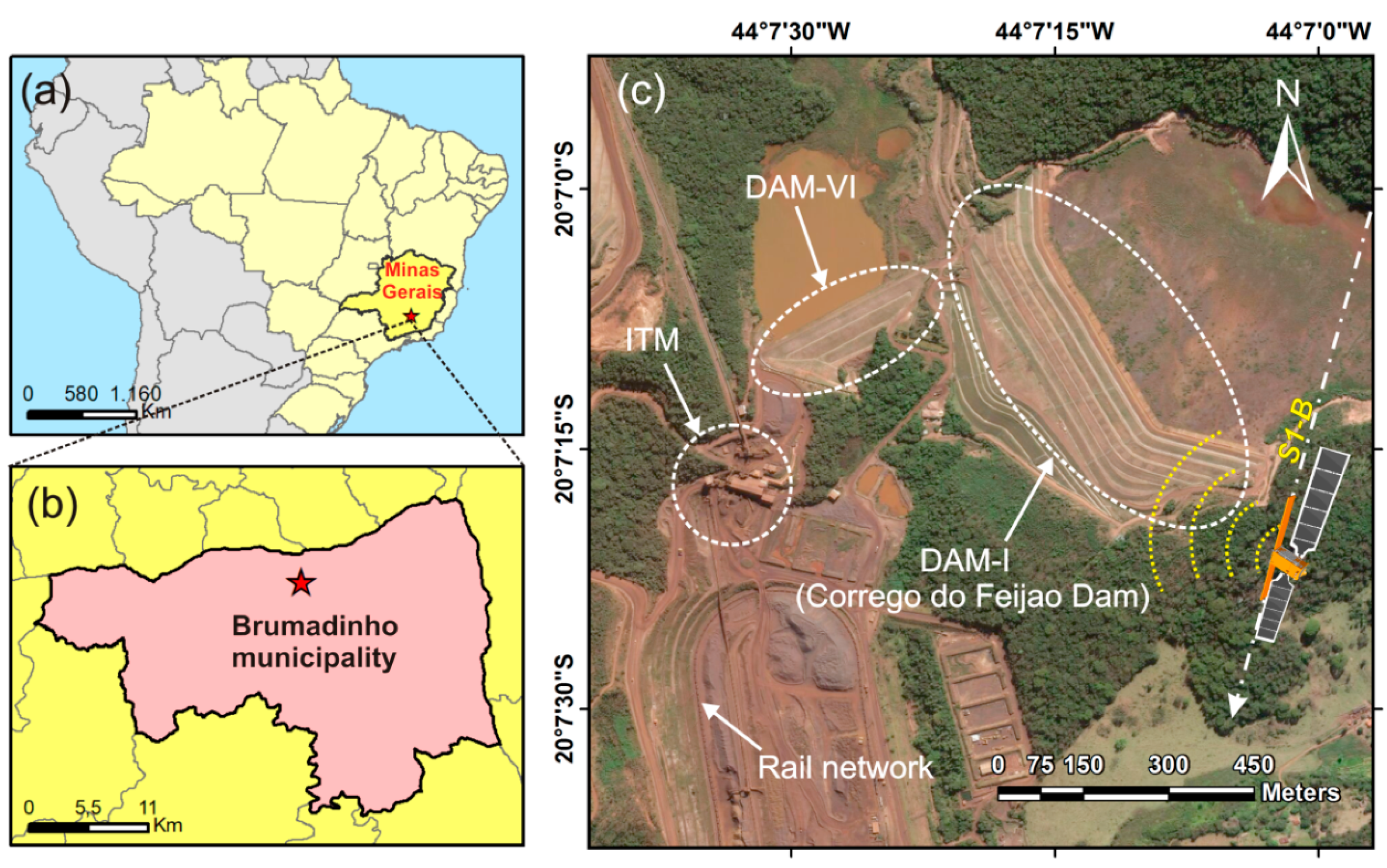
2. The Study Area
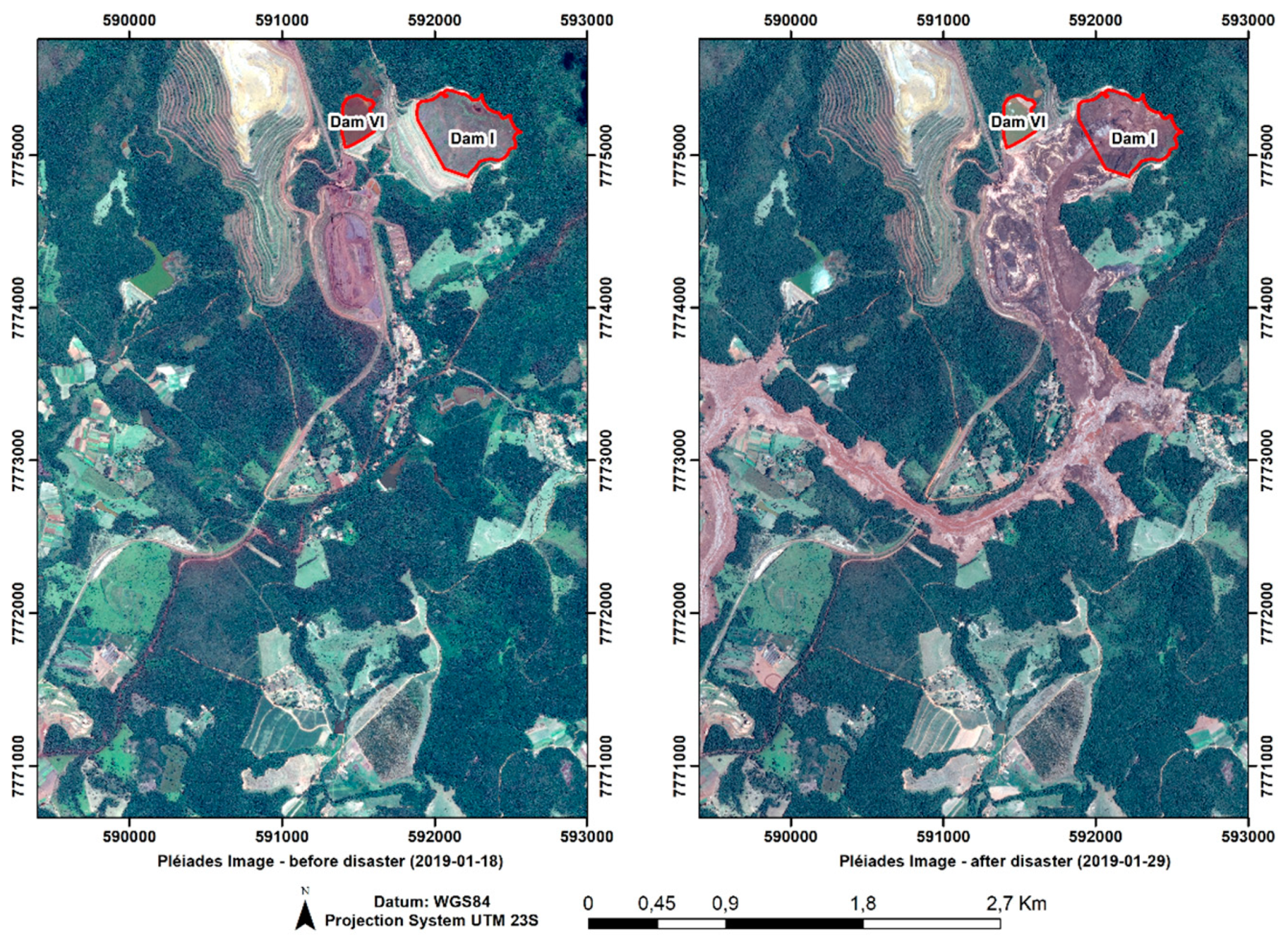
The Dam-I Rupture
3. Materials and Methods
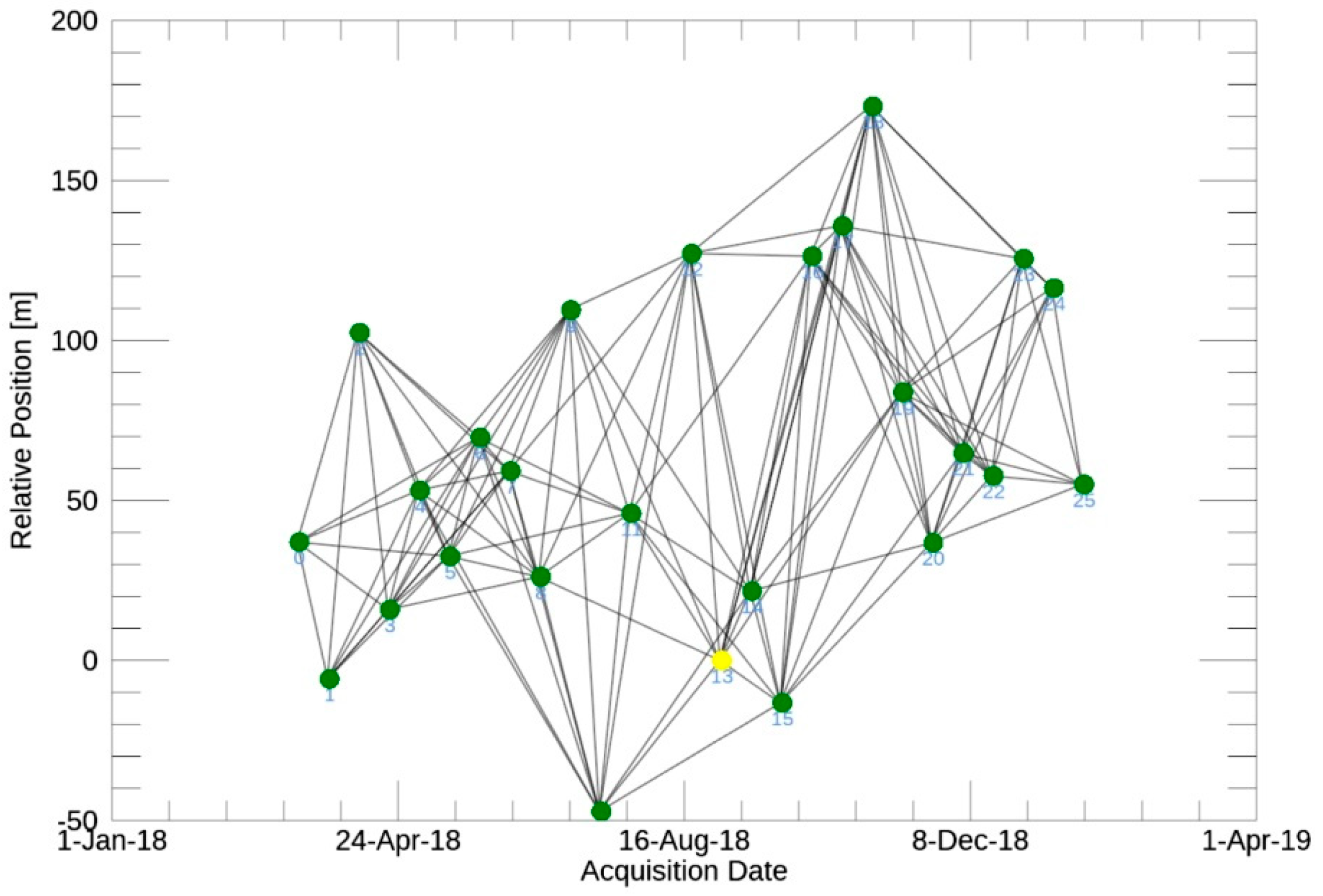
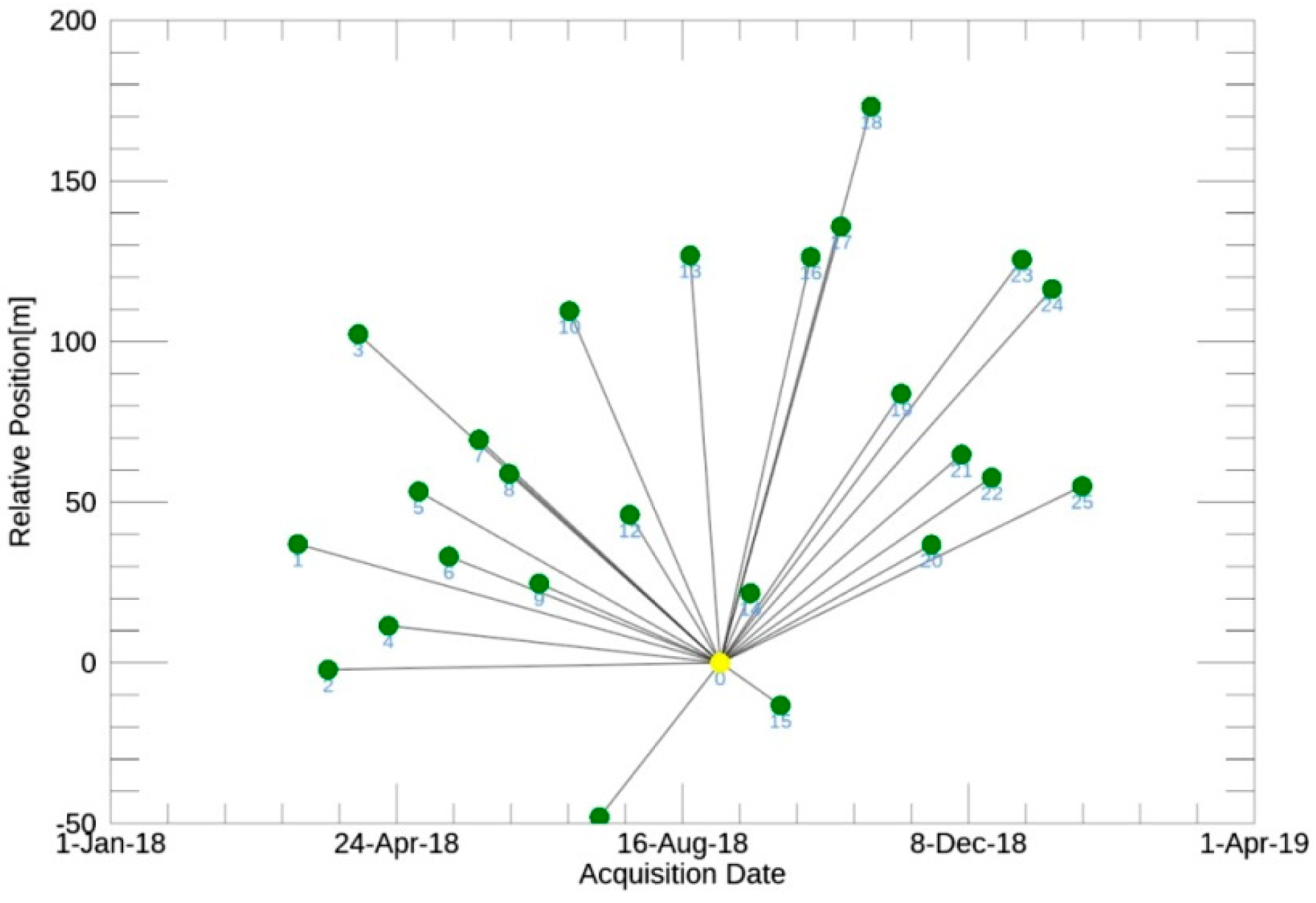
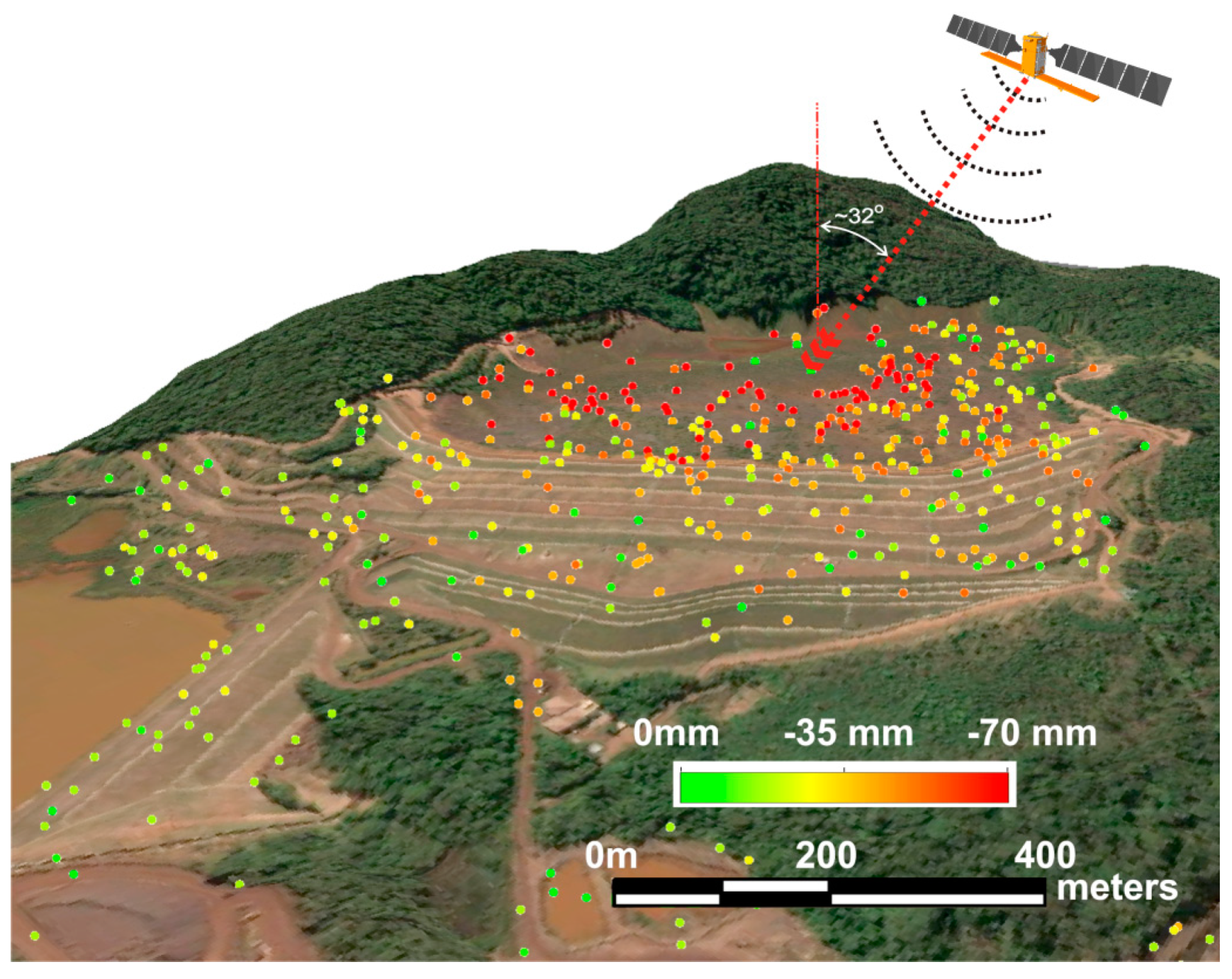
3.1. Satellite Data
3.2. Methodological Approach
3.2.1. DInSAR Analysis
3.2.2. Failure Prediction
4. Results
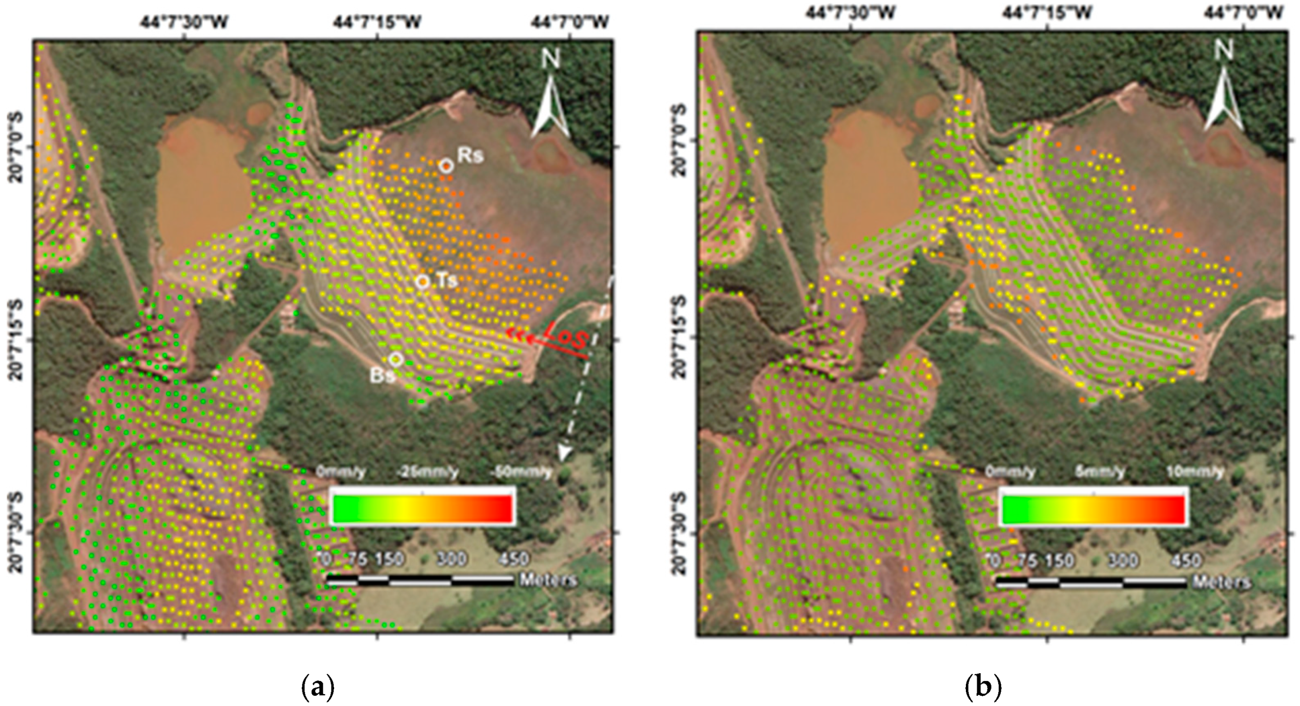
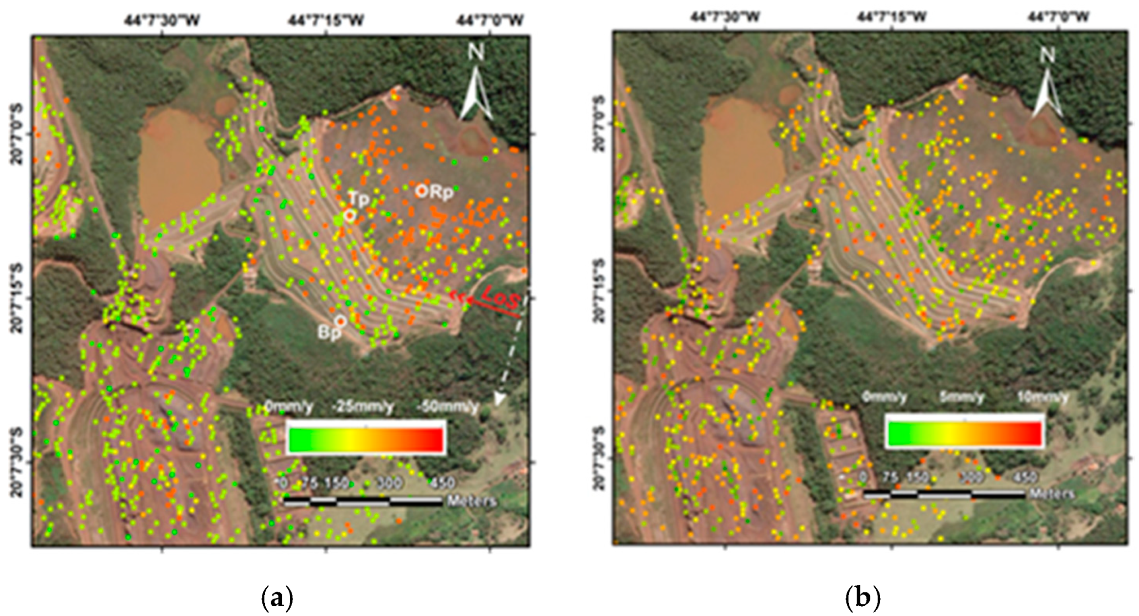
4.1. SBAS Analysis
4.2. PSI Analysis
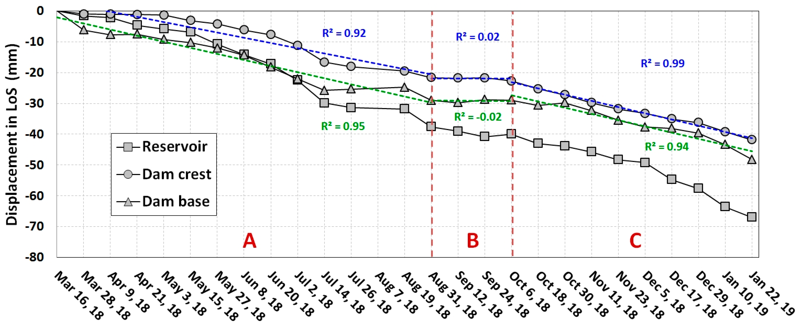
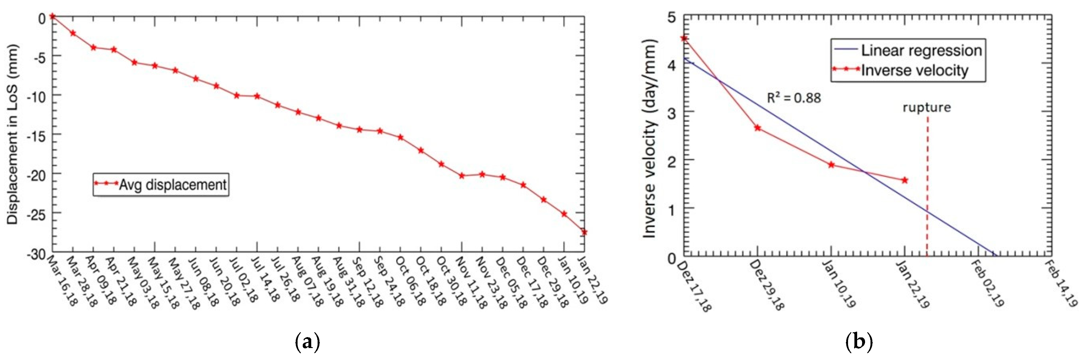
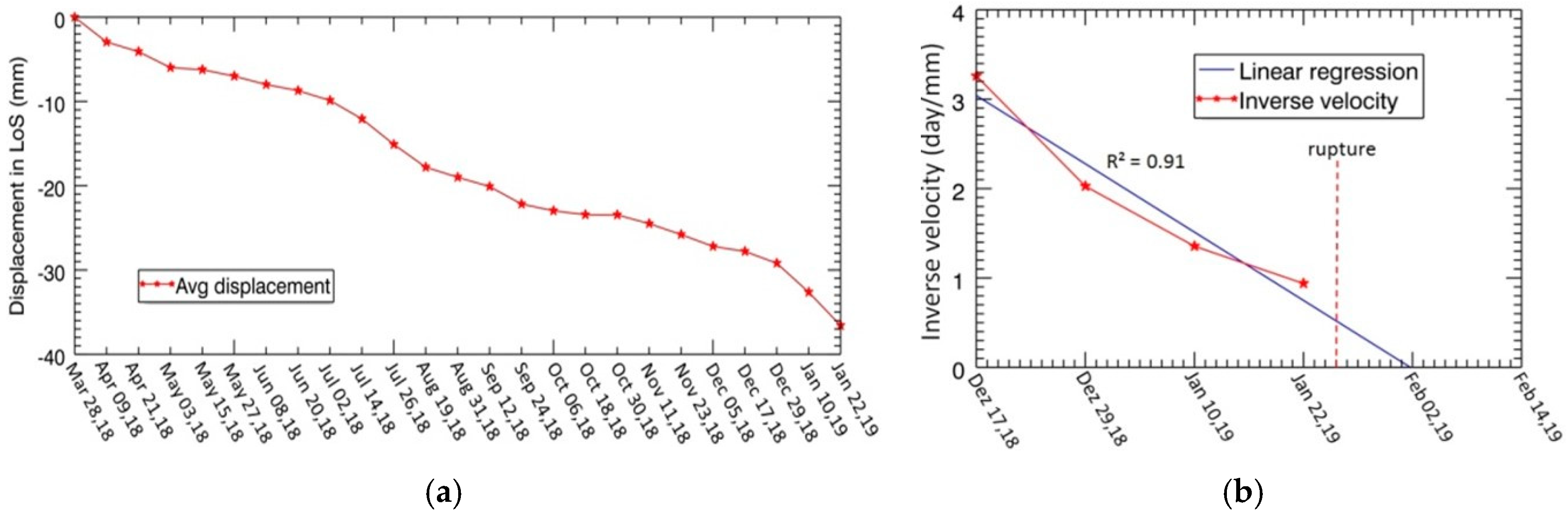
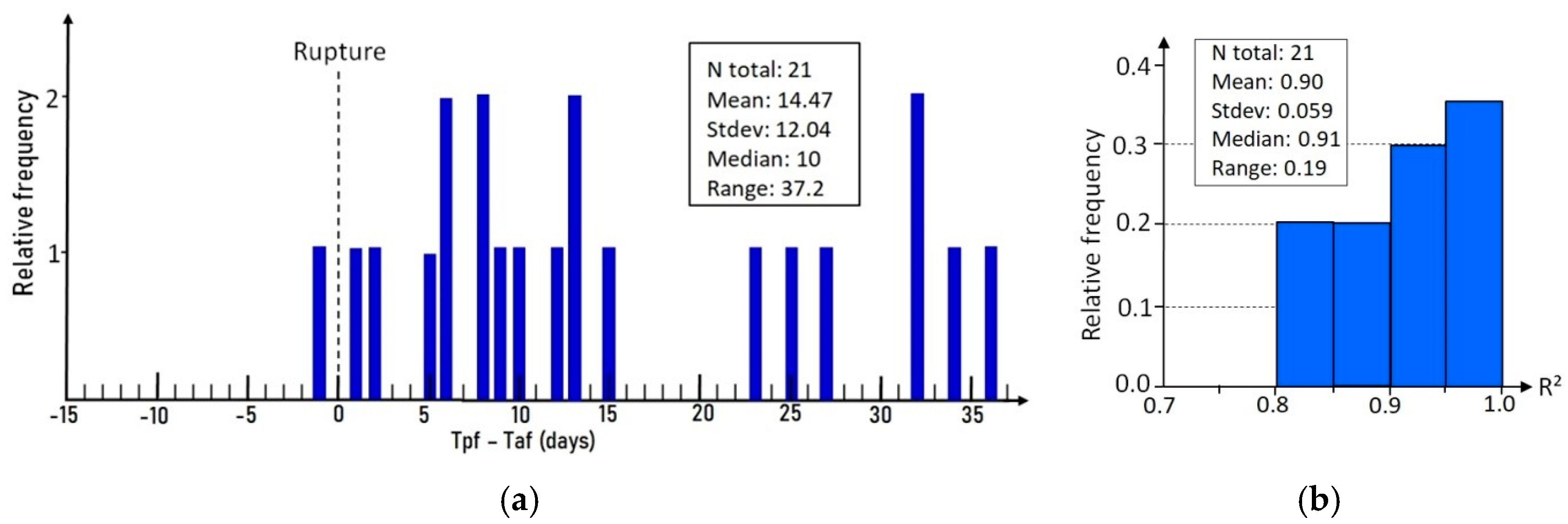
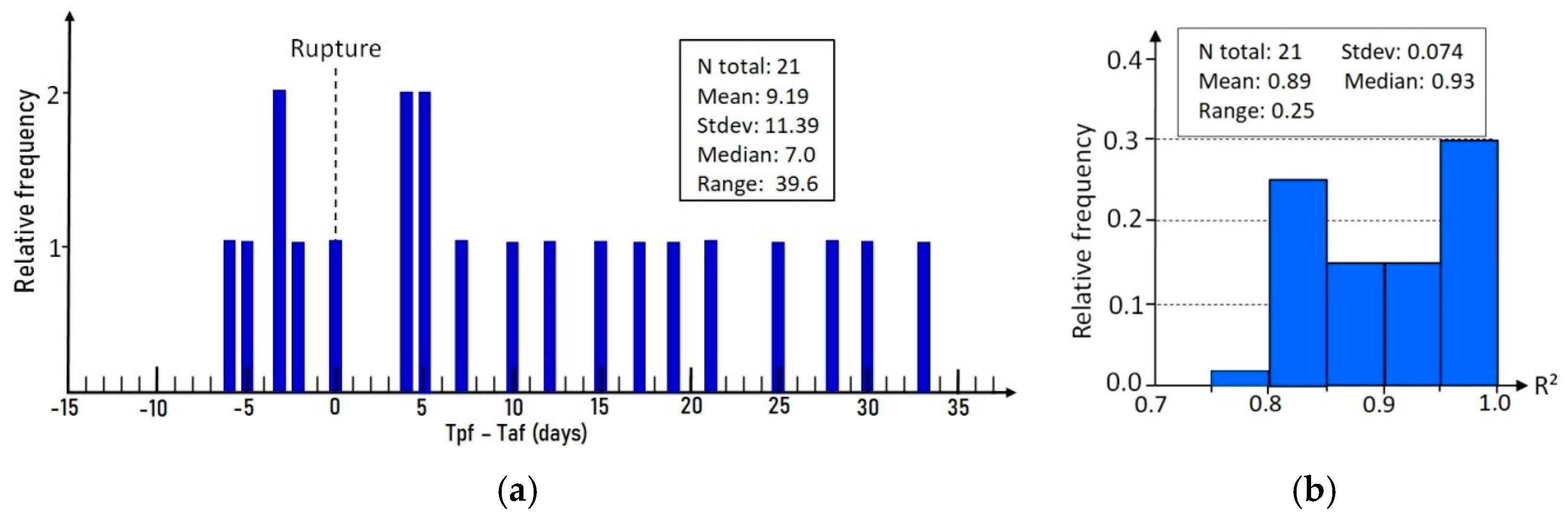
4.3. Failure Prediction Analysis
5. Discussion
6. Conclusions
Author Contributions
Funding
Acknowledgments
Conflicts of Interest
Abbreviations
| DInSAR | Differential Interferometric SAR |
| PSI | Persistent Scatterer Interferometry |
| IPTA | Interferometry Point Target Analysis |
| SBAS | Small BAseline Subset |
| MCF | Minimum Cost Flow |
| SVD | Singular Value Decomposition |
| LoS | Line-of-Sight |
References
- Vale, S.A. Financial Results 2019. Available online: http://Saladeimprensa.vale.com/em/Paginas/Articles.aspx?r=Financial_Results_2019&s=Finance&rID=1323&sID=5 (accessed on 13 March 2020).
- WMTF. World Mining Tailings Failure Brumadinho. 2020 Draft Report. Available online: https://worldminetailingsfailures.org/corrego-do-feijao-tailings-failure-1-25-2019/ (accessed on 14 March 2020).
- ANM Tailings Dam Classification and Safety Plan 2019. Available online: http://www.anm.gov.br/assuntos/barragens/pasta-classificacao-de-barragens-demineracao/plano-de-seguranca-de-barragens (accessed on 9 June 2019).
- Kossoff, D.; Dubbin, W.E.; Alfredsson, M.; Edwards, S.J.; Macklin, M.G.; Hudson-Edwards, K.A. Mine Tailings Dams: Characteristics, Failure, Environmental Impacts, and Remediation. Appl. Geochem. 2014, 51, 229–245. [Google Scholar] [CrossRef] [Green Version]
- Morgenstern, N.R.; Vick, S.G.; Viotti, C.B.; Watts, B.D. Fundão Tailings Dam Review Panel: Report on the Immediate Causes of the Failure of the Fundão Dam; Samarco, S.A., Vale, S.A., Eds.; BHP Brasil Ltd.: Belo Horizonte, Brazil, 2016; p. 76. Available online: http://fundaoinvestigation.com/the-panel-report/ (accessed on 18 May 2018).
- Davies, M.; Martin, T. Mining market cycles and tailings dam incidents. In Proceedings of the 13th International Conference on Tailings and Mine Waste, Banff, AB, Canada, 1–4 November 2009; Available online: http://www.infomine.com/library/publications/docs/Davies2009.pdf (accessed on 31 November 2014).
- Alves, C.; Carneiro, S.; Santos, A. Management of Tailings Dam at Samarco Mineração S.A. Presented at the Brazilian Ministry of Mines and Energy, Brasília, Brazil, 13 December 2017; Available online: http://www.mme.gov.br/documents/20182/5e3fa655-7e22-d835-973e-e3f1f8f83547 (accessed on 7 May 2020). (In Portuguese).
- Hartwig, M.E.; Paradella, W.R.; Mura, J.C. Detection and monitoring of surface motions in active mine in the Amazon region, using persistent scatterer interferometry with TerraSAR-X satellite Data. Remote Sens. 2013, 5, 4719–4734. [Google Scholar] [CrossRef] [Green Version]
- Paradella, W.R.; Ferretti, A.; Mura, J.C.; Colombo, D.; Gama, F.F.; Tamburini, A.; Santos, R.A.; Novalli, F.; Galo, M.; Camargo, P.O.; et al. Mapping surface deformation in open pit iron mines of Carajás Province (Amazon Region) using an integrated SAR analysis. Eng. Geol. 2015, 193, 61–78. [Google Scholar] [CrossRef] [Green Version]
- Mura, J.C.; Paradella, W.R.; Gama, F.F.; Silva, G.G.; Galo, M.; Camargo, P.; Silva, A. Monitoring of Non Linear Ground Movement in an Open Pit Iron Mine Based on an Integration of Advanced DInSAR Techniques Using TerraSAR-X Data. Remote Sens. 2016, 8, 409–427. [Google Scholar] [CrossRef] [Green Version]
- Gama, F.F.; Cantone, A.; Mura, J.C.; Pasquali, P.; Paradella, W.R.; Santos, A.R.; Silva, G.G. Monitoring subsidence of open pit iron mines at Carajás Province based on SBAS interferometric technique using TerraSAR-X data. Remote Sens. Appl. Soc. Environ. 2017, 8, 199–211. [Google Scholar]
- Mura, J.C.; Gama, F.F.; Paradella, W.R.; Negrão, P.; Carneiro, S.; Oliveira, C.G.; Brandão, W.S. Monitoring the vulnerability of the dam and dykes in Germano iron mining after the collapse of the tailings dam of Fundão (Mariana-MG, Brazil) using DInSAR techniques with TerraSAR-X data. Remote Sens. 2018, 10, 1507. [Google Scholar] [CrossRef] [Green Version]
- Gama, F.F.; Paradella, W.R.; Mura, J.C.; Oliveira, C.G. Advanced DInSAR analysis on dam stability monitoring: A case study in the Germano mining complex (Mariana, Brazil) with SBAS and PSI techniques. Remote Sens. Appl. Soc. Environ. 2019, 16, 100267. [Google Scholar] [CrossRef]
- Emadali, L.; Motagh, M.; Haghighi, M.H. Characterizing post-construction settlement of the Masjed-Soleyman embankment dam, Southwest Iran, using TerraSAR-X SpotLight radar imagery. Eng. Struct. 2017, 143, 261–273. [Google Scholar] [CrossRef] [Green Version]
- Milillo, P.; Bürgmann, R.; Lundgren, P.; Salzer, J.; Perissin, D.; Fielding, E.; Biondi, F.; Milillo, G. Space geodetic monitoring of engineered structures: The ongoing destabilization of the Mosul dam, Iraq. Sci. Rep. 2016, 6, 37408. [Google Scholar] [CrossRef] [Green Version]
- Al-Husseinawi, Y.; Li, Z.; Clarke, P.; Edwards, S. Evaluation of the stability of the Darbandikhan Dam after the 12 November 2017 Mw 7.3 Sarpol-e Zahab (Iran–Iraq border) earthquake. Remote Sens. 2018, 10, 1426. [Google Scholar] [CrossRef] [Green Version]
- Rotta, L.H.S.; Alcântara, E.; Park, E.; Negri, R.G.; Lin, Y.N.; Bernardo, N.; Mendes, T.S.G.; Sousa Filho, C.R. The 2019 Brumadinho tailings dam collapse: Possible cause and impacts of the worst human and environmental disaster in Brazil. Int. J. Appl. Earth Obs. Geoinf. 2020, 90, 102119. [Google Scholar] [CrossRef]
- Devanthéry, N.; Crosetto, M.; Monserrat, O.; Cuervas-Gonzales, M.; Crippa, B. Deformation monitoring using Sentinel-1 SAR data. In Proceedings of the 2nd International Electronic Conference on Remote Sensing (SCIforum), 22 March–5 April 2018; Volume 2. online. [Google Scholar] [CrossRef] [Green Version]
- Strozzi, T.; Antonova, S.; Günther, F.; Mätzler, E.; Gonçalo Vieira, G.; Wegmüller, U.; Westermann, S.; Bartsch, A. Sentinel-1 SAR Interferometry for Surface Deformation Monitoring in Low-Land Permafrost Areas. Remote Sens. 2018, 10, 1360. [Google Scholar] [CrossRef] [Green Version]
- Béjar-Pizarro, M.; Notti, D.; Mateos, R.M.; Ezquerro, P.; Centolanza, G.; Herrera, G.; Bru, G.; Sanabria, M.; Solari, L.; Javier Duro, J.; et al. Mapping Vulnerable Urban Areas Affected by Slow-Moving Landslides Using Sentinel-1 InSAR Data. Remote Sens. 2017, 9, 876. [Google Scholar] [CrossRef] [Green Version]
- Lanari, R.; Bonano, M.; Buonanno, S.; Casu, F.; De Luca, C.; Fusco, A.; Manunta, M.; Manzo, M.; Onorato, G.; Zeni, G.; et al. Continental scale SBAS-DInSAR processing for the generation of Sentinel-1 deformation time series within a cloud computing environment: Achieved results and lessons learned. In Proceedings of the EGU General Assembly 2020, 4–8 May 2020. EGU2020-17944. [Google Scholar] [CrossRef]
- Intrieri, E.; Raspini, F.; Fumagalli, A.F.; Lu, P.; Conte, D.C.; Farina, P.; Allievi, J.; Ferretti, A.; Casagli, N. The Maoxian landslide as seen from space: Detecting precursors of failure with Sentinel-1 data. Landslides 2018, 15, 123–133. [Google Scholar] [CrossRef] [Green Version]
- Berardino, P.; Fornaro, G.; Lanari, R.; Sansosti, E. A new algorithm for surface deformation monitoring based on small baseline differential SAR interferograms. IEEE Trans. Geosci. Remote Sens. 2002, 40, 2375–2383. [Google Scholar] [CrossRef] [Green Version]
- Ferretti, A.; Prati, C.; Rocca, F. Permanent scatterers in SAR interferometry. IEEE Trans. Geosci. Remote Sens. 2001, 39, 8–20. [Google Scholar] [CrossRef]
- Werner, C.; Wegmuller, U.; Strozzi, T.; Wiesmann, A. Interferometric point target analysis for deformation mapping. In Proceedings of the IEEE International Geoscience and Remote Sensing Symposium (IGARSS 2003), Toulouse, France, 21–25 July 2003; Volume 7, pp. 4362–4364. [Google Scholar]
- Hooper, A.; Zebker, H.; Segall, P.; Kampes, B. A new method for measuring deformation on volcanoes and other natural terrains using InSAR Persistent Scatterers. Geophys. Res. Lett. 2004, 31, L23611. [Google Scholar]
- Carlá, T.; Intrieri, E.; Di Traglia, F.; Nolesini, T.; Gigli, G.; Casagli, N. Guidelines on the use of inverse velocity method as a tool for setting alarm thresholds and forecasting landslides and structure collapses. Landslides 2017, 14, 517–534. [Google Scholar] [CrossRef] [Green Version]
- Carlá, T.; Farina, P.; Intrieri, E.; Botsialas, K.; Casagli, N. On the monitoring and early-warning of brittle slope failures in hard rock masses: Examples from an open-pit mine. Eng. Geol. 2017, 228, 71–81. [Google Scholar] [CrossRef]
- Carlà, T.; Intrieri, E.; Raspini, F.; Bardi, F.; Farina, P.; Ferretti, A.; Colombo, D.; Novali, F.; Casagli, N. Perspectives on the prediction of catastrophic slope failures from satellite InSAR. Sci. Rep. 2019, 9, 14137. [Google Scholar] [CrossRef]
- Sanglard, J.; Rosière, C.A.; Santos, J.O.S.; Mcnaughton, N.J.; Fletcher, I. The structure of the western segmento of Serra do Curral, Iron Quadrangle and the tectonic control of the compact accumulation of iron high content. Geol. USP-Sci. Ser. 2014, 13, 81–95. (In Portuguese) [Google Scholar] [CrossRef]
- Rosière, C.A.; Rolim, V.K. Iron formation and associated high-grade iron ore: The iron ore of Brazil, geology, metallogenesis and economy. In Mineral Resources in Brazil, Problems and Challenges; Brazilian Academy of Sciences: Rio de Janeiro, Brazil, 2016; pp. 2–45. (In Portuguese) [Google Scholar]
- Cavallini, M. The Mine that Hosts the Brumadinho Dams Responds for 2% of Vale Iron Production, Veja Raio-X. 2019. Available online: https://g1.globo.com/economia/noticia/2019/01/28/mina-queabriga-barragem-em-brumadinho-responde-por-2-da-producao-da-vale-veja-raio-x.ghtml (accessed on 28 January 2019).
- Cionek, V.M.; Alves, G.H.Z.; Tófoli, R.M.; Rodrigues-Filho, J.L.; Dias, R.M. Brazil in the mud again: Lessons not learned from Mariana dam collapse. Biodivers. Conserv. 2019, 28, 1935–1938. [Google Scholar] [CrossRef]
- Porsani, J.L.; Jesus, F.A.N.; Stangari, M.C. GPR survey on an iron mining area after the collapse of the tailings dam I at the Córrego do Feijão mine in Brumadinho-MG, Brazil. Remote Sens. 2019, 11, 860. [Google Scholar] [CrossRef] [Green Version]
- Robertson, P.K.; Melo, L.; Williams, D.J.; Wilson, G.W. Report of the Expert Panel on the Technical Causes of the Failure of Feijão Dam 1. 2019, p. 71. Available online: https://bdrb1investigationstacc.z15.web.core.windows.net/assets/Feijao-Dam-I-Expert-Panel-Report-ENG.pdf (accessed on 3 January 2020).
- Osmanoglu, R.; Sunar, F.; Wdowinski, S.; Cabral-Cano, E. Time Series Analysis of InSAR data: Methods and trends. ISPRS J. Photogramm. Remote Sens. 2016, 115, 90–102. [Google Scholar]
- SARscape Technical Description. Available online: http://www.sarmap.ch/pdf/SARscapeTechnical.pdf (accessed on 5 July 2020).
- Lanari, R.; Mora, O.; Manunta, M.; Mallorquí, J.J.; Berardino, P.; Sansosti, E. A small-baseline approach for investigating deformations on full-resolution differential SAR interferograms. IEEE Trans. Geosci. Remote Sens. 2004, 42, 1377–1386. [Google Scholar] [CrossRef]
- Crosetto, M.; Monserrat, O.; Cuervas-Gonzales, M.; Devanthéry, N.; Crippa, B. Persistent Scatterer Interferometry: A review. ISPRS J. Photogramm. Remote Sens. 2016, 115, 79–89. [Google Scholar] [CrossRef] [Green Version]
- Kampes, B.M. Radar Interferometry: Persistent Scatterer Technique; Springer: Berlin/Heidelberg, Germany, 2006. [Google Scholar]
- Wegmuller, U.; Werner, C.; Strozi, T.; Wiesmann, A.; Frey, O.; Santoro, M. Sentinel-1 Support in the GAMMA Software. Procedia Comput. Sci. 2016, 100, 1305–1312. [Google Scholar] [CrossRef] [Green Version]
- Voight, B. A relation to describe rate-dependent material failure. Science 1989, 243, 200–203. [Google Scholar] [CrossRef] [Green Version]
- Petley, D.N.; Bulmer, M.H.; Murphy, W. Patterns of movement in rotational and translational landslides. Geology 2002, 30, 719–722. [Google Scholar] [CrossRef]
- Rose, N.D.; Hungr, O. Forecasting potential rock slope failure in open pit mines using the inverse-velocity method. Int. J. Rock Mech. Min. Sci. 2007, 44, 308–320. [Google Scholar] [CrossRef]
- Dick, G.J.; Eberhardt, E.; Cabrejo-Liévano, A.G.; Stead, D.; Rose, N.D. Development of an early-warning time-of-failure analysis methodology for open-pit mine slopes utilizing ground-based slope stability radar monitoring data. Can. Geotech. J. 2014, 52, 515–552. [Google Scholar] [CrossRef]
- Ministry of Economy (ME). Analysis Report of the Work Accident on the Dam-1 Failure in Brumadinho (MG). 2019; 237p. Available online: https://sit.trabalho.gov.br (accessed on 30 July 2020).
- Leoni, L.; Coli, N.; Farina, P.; Coppi, F.; Michelini, A.; Costa, T.A. On the Use of Ground-Based Synthetic Aperture Radar for Long-Term Slope Monitoring to Support the Mine; Geotechnical Team, Australian Centre for Geomechanics: Perth, Australia, 2015; pp. 789–797. Available online: https://papers.acg.uwa.edu.au/p/1508-58-Farina (accessed on 10 July 2020).
- Michelini, A.; Farina, P.; Coli, N.; Coppi, F.; Leoni, L.; Sá, G.; Costa, T. Advanced Data Processing of ground-based Synthetic Aperture Radar for slope monitoring in open pit mines. In Proceedings of the 48th US Rock Mechanics Geomechanics Symposium, Minneapolis, MN, USA, 1–4 June 2014; Available online: https://www.researchgate.net/publication/282699042 (accessed on 30 July 2020).


| Acquisition | Date | Acquisition | Date |
|---|---|---|---|
| 1 | 20180316 | 14 | 20180831 |
| 2 | 20180328 | 15 | 20180912 |
| 3 | 20180409 | 16 | 20180924 |
| 4 | 20180421 | 17 | 20181006 |
| 5 | 20180503 | 18 | 20181018 |
| 6 | 20180515 | 19 | 20181030 |
| 7 | 20180527 | 20 | 20181111 |
| 8 | 20180608 | 21 | 20181123 |
| 9 | 20180620 | 22 | 20181205 |
| 10 | 20180702 | 23 | 20181217 |
| 11 | 20180714 | 24 | 20181229 |
| 12 | 20180726 | 25 | 20190110 |
| 13 | 20180819 | 26 | 20190122 |
| SBAS: Crest (Ts) | SBAS: Bottom (Bs) | |
|---|---|---|
| Sector A | −50.71 mm/y | −25.25 mm/y |
| Sector B | −13.78 mm/y | −2.74 mm/y |
| Sector C | −48.07mm/y | −60.59 mm/y |
| PSI: Crest (Tp) | PSI: Base (Bp) | |
|---|---|---|
| Sector A | −46.97 mm/y | −63.08 mm/y |
| Sector B | −11.48 mm/y | −0.84 mm/y |
| Sector C | −64.49 mm/y | −65.10 mm/y |
© 2020 by the authors. Licensee MDPI, Basel, Switzerland. This article is an open access article distributed under the terms and conditions of the Creative Commons Attribution (CC BY) license (http://creativecommons.org/licenses/by/4.0/).
Share and Cite
F. Gama, F.; Mura, J.C.; R. Paradella, W.; G. de Oliveira, C. Deformations Prior to the Brumadinho Dam Collapse Revealed by Sentinel-1 InSAR Data Using SBAS and PSI Techniques. Remote Sens. 2020, 12, 3664. https://doi.org/10.3390/rs12213664
F. Gama F, Mura JC, R. Paradella W, G. de Oliveira C. Deformations Prior to the Brumadinho Dam Collapse Revealed by Sentinel-1 InSAR Data Using SBAS and PSI Techniques. Remote Sensing. 2020; 12(21):3664. https://doi.org/10.3390/rs12213664
Chicago/Turabian StyleF. Gama, Fábio, José C. Mura, Waldir R. Paradella, and Cleber G. de Oliveira. 2020. "Deformations Prior to the Brumadinho Dam Collapse Revealed by Sentinel-1 InSAR Data Using SBAS and PSI Techniques" Remote Sensing 12, no. 21: 3664. https://doi.org/10.3390/rs12213664