Fuel Type Classification Using Airborne Laser Scanning and Sentinel 2 Data in Mediterranean Forest Affected by Wildfires

Abstract

Mediterranean forests are recurrently affected by fire. The recurrence of fire in such environments and the number and severity of previous fire events are directly related to fire risk. Fuel type classification is crucial for estimating ignition and fire propagation for sustainable forest management of these wildfire prone environments. The aim of this study is to classify fuel types according to Prometheus classification using low-density Airborne Laser Scanner (ALS) data, Sentinel 2 data, and 136 field plots used as ground-truth. The study encompassed three different Mediterranean forests dominated by pines (Pinus halepensis, P. pinaster y P. nigra), oaks (Quercus ilex) and quercus (Q. faginea) in areas affected by wildfires in 1994 and their surroundings. Two metric selection approaches and two non-parametric classification methods with variants were compared to classify fuel types. The best-fitted classification model was obtained using Support Vector Machine method with radial kernel. The model includes three ALS and one Sentinel-2 metrics: the 25th percentile of returns height, the percentage of all returns above mean, rumple structural diversity index and NDVI. The overall accuracy of the model after validation was 59%. The combination of data from active and passive remote sensing sensors as well as the use of adapted structural diversity indices derived from ALS data improved accuracy classification. This approach demonstrates its value for mapping fuel type spatial patterns at a regional scale under different heterogeneous and topographically complex Mediterranean forests.

1. Introduction

Wildfires constitute a recurrent hazard in forested environments around the world, shattering many environmental and socio-economic resources each year. Fires shape the current landscape in the Mediterranean basin [1] modifying forest structure, composition and species richness [2]. An average of 45,000 fires is recorded yearly [3] in the Mediterranean region, with Spain being the second most affected country after Portugal [4]. For example, in 1994, 327,696 ha were burned due to an extreme dry summer and high temperatures, and was one of the most affected years reported by the Spanish fire database [5]. Forest fire risk mitigation is under the spotlight due to uncertain effects of climate and socioeconomic changes [6] pushing firefighting agencies to increase their funding, as for example up to 78 million € in 2015 in Spain (MAPAMA).

Forest managers need to evaluate fire risk [7], which is a critical and difficult hazard to manage since fuel distributions change [8]. Furthermore, fire ignition and propagation include several drivers (i.e., fuel moisture, weather and wind conditions, topography) [9]. Fuel quantity and distribution are the only drivers that managers can control, which make fuel mapping critical to improve fire danger assessment and fire behavior modelling [10]. The characterization and mapping of vegetation fuels can be approached either by determining the different fuel properties (i.e., surface and/or crown properties) or by mapping fuel types [10]. The term fuel types refers to an identifiable association of fuel elements, of different species, form, size, arrangement and continuity, with similar predictable fire behavior under defined burning conditions [11]. Generally, fuel types are grouped into vegetation classes with a similar predicted fire behavior according to their height and fuel density [12]. Several fuel type classifications have been proposed within the literature. The most commonly used where developed in USA and Canada such as the classifications from Anderson [13], Sandberg et al. [14], the widely used by the Northern Forest Fire Laboratory (NFFL) proposed by Albini [15] or the Canadian Fire Behavior Prediction (FBP) System [16]. An adaptation from NFFL system, which considers the Rothermel fire spread model, to the Mediterranean basin conditions was performed by the Prometheus project [17] as several authors pointed out that each fuel type classification is only applicable to similar geographic and environmental conditions. Prometheus fuel system was chosen for being specifically designed to better adapt to fuels found in Mediterranean ecosystems and its classification with remote sensing techniques [18,19]. Furthermore, Prometheus considers height and density of propagators elements as the main drivers in fire behavior, being LiDAR data especially useful for deriving these fuel characteristics [18]. This classification of fuel models considers height and density of propagators elements as the main drivers in fire behavior.

The mapping of fuel properties and fuel types have been historically carried out based on field surveys, which are challenging and expensive [12]. The main advantage of field surveys is the limited error, being currently used to create field reference datasets, while the difficulty in time and cost is evident for operational fuel characterization [18]. Remote sensing can assist fuel mapping through the characterization of horizontal and vertical forest structure components [20] providing the necessary temporal, spectral and spatial coverage, while being less time-consuming than field surveys or aerial photo interpretation [12]. Several studies have attempted fuel type or properties mapping using passive multispectral remote sensing images [19,21,22,23] and similar levels of accuracy were found between the use of medium-resolution sensors and very high-resolution ones according to Arroyo et al. [18]. Although little comparison has been carried out between the use of multispectral and hyperespectral data, Lasaponara et al. [24] determined an increase of around 20% of the overall accuracy when classifying Prometheus fuel types with MIVIS respect to Landsat TM. However airborne hyperspectral data are generally limited to the reduced spatial coverage that they provide [18]. The most relevant limitation of passive remote sensing data is their inability to penetrate forest canopies as well as their indirect relationship with vertical structure [20]. In this sense, active sensors such as Synthetic Aperture Radar (SAR) [25,26], and specially LIDAR constitute an alternative in order to vertical forest structure characterization [27,28]. The integration of multispectral and LiDAR data has been recognized as a suitable approach to improve fuel characterization. For example, Alonso-Benito et al. [29] reported an improvement of 10% of the overall accuracy when combining World View-2 and LiDAR data, and Mutlu et al. [8] pointed out an improvement of 14% when combining QuickBird and LiDAR data.

According to Ferraz et al. [10], direct and indirect approaches have been proposed to map fuels using ALS or its integration with spectral information. The direct approach intends to determine and characterize surface and crown fuel properties, while the indirect one classifies the forest fuels in terms of Fuel types. Several studies have focused on the direct approach to estimate fuel properties using ALS data [30,31,32,33,34,35,36,37,38], or integrating ALS and spectral information [27,39,40]. Furthermore, the characterization of fuel properties, and subsequent prediction of fire behavior was also attempted by Botequim et al. [41] and Sánchez et al. [42]. Some studies have explored the indirect fuel type mapping approach integrating ALS data with high-resolution multispectral images [8,29,43], with middle resolution passive sensors [44,45], its combination with SAR data [46] or ALS data alone [12], obtaining better results those that combine multi source datasets. The use of ALS data is particularly relevant for characterizing the vertical structure of fuel types as well as to discriminate fuel discontinuities [45]. Studies that have mapped fuel type have selected either a suite of statistical metrics commonly used for forestry applications, related to height distribution and canopy cover at different heights [44] or applying the height bin approach [8]. The height bin approach computes the proportion of ALS returns within different height ranges creating a 3D vegetation vertical profile. The use of structural metrics proposed to assess forest structure complexity such as rumple [47] or forest structural diversity as LiDAR height diversity index (LHDI), and LiDAR height evenness index (LHEI) [48], might help to create parsimonious models. Concerning the training sample in fuel type modelling using ALS data, two approaches can be found in previous studies; regional studies mostly used previous mapping to train the model [45,46] and more local ones used field plots as sample, usually from low to medium size, between 50 and 100 field plots [8,43,44].

Despite fuel mapping in Mediterranean ecosystems have been previously addressed [28,29], there is a lack of research on the integration of medium-resolution multispectral data with low point density ALS data for fuel types mapping at regional scale. To the best of our knowledge, this is the first attempt to classify fuel types at regional scale using low density ALS data, multispectral Sentinel 2 data, and field work that compares the performance of classification using both datasets together or separately. Sentinel 2 data have been used to characterize canopy fuel characteristics [23], fuel types [49] or mapping wildfire ignition [42], while the integration with ALS for fuel mapping at regional scale requires further analysis. Furthermore, the research analyzes whether differences in the presence of fuel types exists between areas previously burned in 1994 or unburned ones. Different authors have studied the regrowth of fire vegetation after fire [1,50], but the analysis of fuel type composition after fire and its comparison with unburned areas remains unknown in Mediterranean environments, characterized by a high topographic heterogeneity, vegetation species and climate. The study is developed within the SERGISAT project framework, whose aim is the analysis of the effects of fire severity and environmental variables on regeneration of areas affected by large forest fires in Spain, considering fraction cover, biomass and biodiversity.

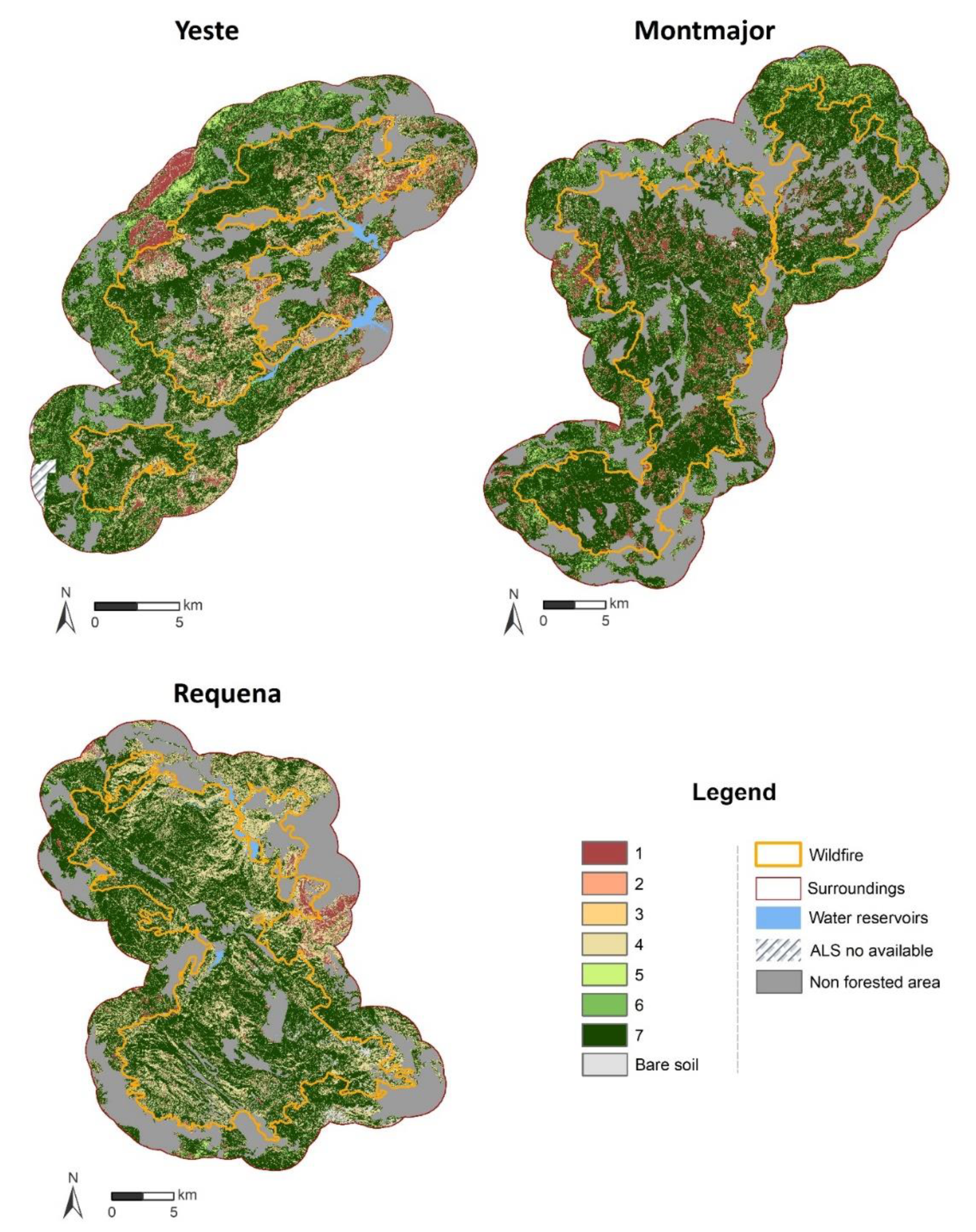
In this context, the aim of this study was to classify and map fuel types according to Prometheus classification using low density ALS data, Sentinel-2A data and field work within three different Mediterranean forests dominated by pines (Pinus halepensis, P. pinaster y P. nigra), oaks (Quercus ilex) and quercus (Q. faginea). Furthermore, the following secondary objectives are addressed: (i) compare classification performance when combining ALS metrics with Sentinel-2 or when using these data sources separately; (ii) characterize fuel type spatial patterns under areas affected by a previous wildfire with high structural heterogeneity, topographical complexity, and different species representative of the Mediterranean region to create an integrated model for the Spanish Mediterranean arch; (iii) compare fuel type presence between burned and un-burned areas; (iv) analyze the use of synthetic ALS derived metrics to integrate structural complexity and diversity for obtaining parsimonious classifications, and depicting its importance in model performance; (v) compare two metric selection approaches and two non-parametric classification methods.

2. Materials and Methods

2.1. Study Area

The forests under study are located in areas affected by three wildfires as well as their surroundings. The wildfires took place in 1994 within the Spanish municipalities of Montmajor, Requena and Yeste at Barcelona, Valencia and Albacete Spanish provinces, respectively (Figure 1). A total of 95,193.93 ha were affected by the fire, but the study area includes a 2.5 km buffer surrounding the wildfire perimeters, summing up a total of 202,300.54 ha.

Montmajor forested site includes 43,774.45 ha affected by fire, and 41,868.91 ha within the surrounding area. Forests are dominated by Quercus faginea, Quercus pubescens and Pinus nigra, accompanied by areas with presence of shrubs dominated by Rosmarinus officinalis, Rubus sp. and Genista scorpius. Pastures where characterized by the presence of Brachipodium sp. while areas with higher water availability where dominated by species such as Hedera helix. Furthermore, recurrence of fire burned 1000 ha in the central west part during 2005. In this area, the annual precipitation ranges from 430 to 890 mm in accordance with Digital Climatic Atlas of the Iberian Peninsula (DCAIP) (http://opengis.uab.es/wms/iberia/en_index.htm), and the average annual temperature is 13 °C. Forests are characterized by a hilly topography, with elevations ranging from 210 to 1240 m above sea level (a.s.l.) and slopes from 12% to higher than 45%. Cenozoic conglomerates, sandstones, clays and limestone dominate the lithology.

Requena forested site includes 38,750.15 ha affected by fire, and 36,884.14 ha within the surrounding area. Forests are mainly dominated by Pinus halepensis, while Pinus pinaster and Quercus ilex rotundifolia are present to a lesser extent. Furthermore, shrubland dominated by Rosmarinus officinalis, Quercus coccifera and Juniperus oxicedrus, and pasture areas characterized by the presence of Brachipodium sp., Ulex parviflorus and Rubia peregrina constitute a relevant land cover. Three fires affected recurrently the analyzed area after being burned in 1994. Two fires affected around 2900 ha in the eastern part in 2000 and 2003, and one small wildfire burned 100 ha in the western part in 2012. In this site, the annual precipitation ranges from 435 to 680 mm (DCAIP), and the average annual temperature is 13 °C. Forests are also characterized by a hilly topography, with elevations ranging from 180 to 1250 m a.s.l. and slope steepness ranging from 13% to higher than 45%. Sandstones and conglomerates from Mesozoic and Cenozoic Era dominate the lithology.

Yeste forested site includes 12,669.33 ha affected by fire, and 28,753.56 ha within the surrounding area. Forests are dominated by Pinus halepensis and, to a lesser extent, Pinus nigra and Pinus pinaster. Shrublands are dominated by Rosmarinus officinalis, Juniperus oxicedrus and Quercus coccifera, while pastures are dominated by Brachipodim sp. and young trees from Quercus constitute the remaining vegetation. In this area, the annual precipitation ranges from 430 to 700 mm (DCAIP), and the average annual temperature is 14 °C. Forests are characterized by a hilly topography, with elevations ranging from 600 to 1670 m a.s.l., and slopes from 16.5% to higher than 50%. The lithology is dominated by dolomites, limestone and marls from Mesozoic Era.

2.2. Field Data

Field data was acquired in 136 field plots from three field campaigns performed during 2017 and 2018. A stratified random sampling technique was selected to establish the location of the field plots, considering a representative sample of terrain slope, aspect, fire severity, dominant pre-fire tree formation, height and cover of the forested areas. To perform this procedure, slope and aspect were derived using ALS data while fire severity was measured using passive remote sensing data from the Landsat archive. Slope and aspect where computed at 10 m resolution by resampling, using the bilinear interpolation in ArcGIS, the digital elevation model (DEM) generated at 1m resolution for ALS metric computation (see Section 2.3. ALS Data and Processing for further details). Fire severity was computed, within the SERGISAT project [51,52], using a simulation method based on the Composite Burn Index [53], called GeoCBI [54].

The Spanish Forest Map adapted by Rodrigues et al. [55] was used to determine pre-fire forest types and the height and cover of vegetation was derived from the ALS point cloud (see Section 2.3. ALS Data and Processing for information on data source and processing) to define homogeneous areas. Furthermore, road and path accessibility were checked to avoid inaccessible areas. A Leica VIVA^® GS15 CS10 GNSS real-time kinematic Global Positioning System was used to locate the centroid of the circular plots, which presented a variable radius of 5, 10 or 15 m. Plots with lower radii were mainly associated to homogeneous areas where really high tree or shrub covers, associated to post-fire regrowth processes, made difficult to move within the plot. Prometheus classification fuel type was in situ identified in each plot, determining one of the seven different fuel classes described in

Table 1. Fuel types defined by Prometheus classification.

Fuel Type	Cover	Shrub Mean Height		Difference between Shrubs and Trees
FT1	>60% grass
FT2	>60% shrub and <50% trees (>4 m)		0.30–0.60 m
FT3			0.60–2.00 m
FT4			2.00–4.00 m
FT5	<30% shrub and >50% trees (>4 m)
FT6	>30% shrub and >50% trees (>4 m)			>0.5 m
FT7				<0.5 m

. An additional class was added to account for those areas without vegetation, named bare soil. Four photos in each of the cardinal points from the centroid of the plots were taken. Furthermore, the slope, elevation, flora inventory, tree and shrub characterization of height and cover, date and hour of acquisition were recorded.

Table 2. Number of plots per fuel type collected during the field campaigns in 2017 and 2018. Fuel type refers to Prometheus fuel type. BS stands for bare soil.

Wildfire	BS	Fuel Type 1	Fuel Type 2	Fuel Type 3	Fuel Type 4	Fuel Type 5	Fuel Type 6	Fuel Type 7	Total
Montmajor	3	3	2	8	1	8	11	11	47
Requena	2	3	9	9	15	2	11	15	66
Yeste	3	3	2	1	4	0	7	3	23
Total	8	9	13	18	20	10	29	29	136

include the number of field plot sampled by wildfire and fuel type.

2.3. ALS Data and Processing

The ALS data were acquired by the Spanish National Plan for Aerial Orthophotography (PNOA) between 2015 and 2016 using a Leica ALS80 discrete-return sensor operating at a wavelength of 1064 nm. Average flying altitude was 3150 m a.s.l. with a maximum scan angle of up to 25° from nadir. The sensor used an average pulse repetition frequency of 230 KHz, average scanning frequency of 43.5 Hz and the average RMSE in z values obtained was 0.09 m. Point clouds were provided in 2 × 2 km tiles in LAS format in European Terrestrial Reference System (ETRS) 1989 Universal Transverse Mercator (UTM) with up to four return per pulse.

The processing of ALS point clouds started with the removal of noise points and overlapping returns, as the existence of vertical (z) or horizontal (x, y) displacements were found between flight lines by visual verification. The 699 tiles that cover the three areas affected by wildfires were filtered using the multiscale curvature classification algorithm [56] according to Montealegre et al. [57], implemented in MCC 2.1 command-line tool. The Point-Triangulated Irregular Network-Raster interpolation method [58] was selected according to Montealegre et al. [59] to generate a digital elevation model (DEM) with a 1-m grid resolution using ArcGIS 10.5 software. The point clouds were clipped to the spatial extent of the field plots and return heights were normalized by subtracting the DEM heights using FUSION LDV 3.60 open source software [60].

A full suite of statistical metrics, commonly used within forestry, related to height distribution and canopy density cover were computed (

Table A1. Statistical metrics derived from the ALS point cloud.

Group	Metric	Acronym
Canopy height metrics (CHM)	Percentiles of the return heights 1, 5, 10, 20, 25, 30, 40, 50, 60, 70, 75, 80, 90, 95 and 99	P01, P05, …,P99
	Minimum elevation	Elev.min
	Maximum elevation	Elev.max
	Mean elevation	Elev.mean
	Mode elevation	Elev.mode
	Elevation quadratic mean	Elev. SQRT mean SQ
	Elevation cubic mean	Elev. CUR mean CUBE
	L moments ($\mathsf{\lambda }$1 to $\mathsf{\lambda }$4)	Elev. L1, Elev. L2, Elev. L3, Elev. L4
	Maximum elevation
Canopy height variability metrics (CHVM)	Standard deviation of point height distribution	Elev. SD
	Variance of point height distribution (σ2)	Elev.variance
	Coefficient of variation of point height distribution	Elev.CV
	Skewness of point height distribution	Elev.skewness
	kurtosis of point height distribution	Elev.kurtosis
	Interquartile distance of point height distribution	Elev.IQ
Canopy density metrics (CDM)	Percentage of first returns above a height-break, above the mean or the mode	e.g., % first ret. Above 0.20
	Percentage of all returns above a height-break, above the mean or the mode	e.g., % all ret. Above mean
	Percentage of all returns with a range of 0.5 m	e.g., % all ret. between 1 and 1.5 m
	Canopy relief ratio	CRR
	All returns above a height-break, above the mean or the mode x 100	e.g., (All ret. Above 0.20)/(total first ret.) by 100
	Percentage of returns between 0.2 m and 95th percentile according to Næsset (2004)	D0, D1, D2, D3, D4, D5, D6, D7, D8, D9
Diversity indices	Foliage Height Diversity Index or height diversity index	LHDI_regular, LHDI_Prometheus
	LiDAR height evenness index	LHEI_regular, LHEI_Prometheus
	Rumple index	Rumple

Appendix A). A threshold value of 0.2 m height was applied, considering the RMS in z values of ALS-PNOA data, to remove ground and understory returns. Canopy height metrics includes percentiles at different intervals (P01, P05, P10, P20, P30, P40, P50, P60, P70, P75, P80, P90, P95, P99), minimum, maximum, median, mode (Elev.min, Elev.max, Elev.mean, Elev.mode), quadratic and cubic elevation (Elev. SQRT mean SQ, Elev. CUR mean CUBE) and L moments (Elev. L1, Elev. L2, Elev. L3). Canopy height variability computed metrics include standard deviation (Elev. SD), variance (Elev.variance), coefficient of variation (Elev.CV), interquartile distance (Elev.IQ), skewness (Elev.skewness) and kurtosis (Elev.kurtosis). Canopy cover metrics include canopy relief ratio (CRR), percentage of first or all returns above a threshold, the mean or the mode (e.g., % first ret. Above 0.20), percentage of all returns with a range of 0.5 m (e.g., % all ret. between 1 and 1.5 m), the ratio of all returns respect to the number of total returns (e.g., (All ret. Above 0.20)/(total first ret.) by 100), and the percentage of points of 10 equally distributed vertical layers derived by dividing the height between the 95th percentile of the height distribution and the 0.2 m threshold (D0, D1,…, D9) [60,61].

Three structural diversity indices were also computed. The LHDI [48] or also called Foliage Height Diversity Index [62,63] which is an adaptation of the Shannon (H’) index (Equation (1)). The LHEI proposed by Listopad et al. [48] that adapts the Pielou (J´) index (Equation (2)), and rumple index [47] as a measure of rugosity or structural heterogeneity (Equation (3)).

$$LHDI=-{\displaystyle \sum }\left[\left(p_h\right)\times ln\left(p_h\right)\right]$$

(1)

$$LHEI=\frac{LHDI}{ln\left(p_h\right)}$$

(2)

$$Rumple=\frac{3D canopy surface model area}{ground area}$$

(3)

where p is the proportion of returns at regular intervals of 0.5 m or at defined Prometheus classification height intervals (h).

The first step to compute LHDI and LHEI was the calculation of return proportion at regular intervals of 0.5 m according to Listopad et al. [48] (“LHDI_regular” and “LHEI_regular”). Furthermore, the indexes were computed using the Prometheus classification height ranges intervals at: 0.2 m, 0.6 m, 2.0 m and 4.0 m [64] (“LHDI_Prometheus” and “LHEI_Prometheus”.

Rumple index is the ratio of three-dimensional canopy surface model (CSM) to ground area. Rumple was computed as the ratio between the sum of the three-dimensional area of triangles from CSM grid points to the two-dimensional area of the grid cell surface. The CSMs were created for each plot using a 1.5 m pixel and a 3 × 3 smoothing algorithm, considering point cloud density of LiDAR-PNOA. The surface area of each CSM 1.5 m pixel is computed by creating triangles that fit the centroid of the pixel and those of the neighboring ones [47]. CSMs were created using the highest returns of each height range to account for canopy rugosity. Rumple was computed for Prometheus classification height ranges (0.2, 2 and 4) to characterize heterogeneity within each stratum, and for the forest canopy including the range between 0.2 up to 40 m.

2.4. Sentinel Data and Processing

Nineteen cloud-free images from the medium-high spatial resolution Sentinel-2A/B MSI sensor were used to cover the variability within the vegetative period for the three wildfires and their surrounding area under study (

Table 3. Selected Sentinel-2 cloud-free images for the three wildfires and their surrounding areas used for generating the composite.

Wildfire	Dates	Tile
Montmajor	07-07-2016, 17-07-2016 *, 30-07-2016, 26-08-2016 *, 28-09-2016 *	31TCG, 31TDG
Requena	10-07-2016, 30-07-2016 *, 09-08-2016, 18-08-2016, 19-08-2016 *	30TXK, 30SXJ
Yeste	23-06-2016, 03-07-2016, 02-08-2016, 22-08-2016	30SWH

* stands for images that were captured in the same day within different tiles.

). The images were downloaded from the European Space Agency’s (ESA) Sentinel Scientific Data Hub (https://scihub.copernicus.eu/) with a processing Level-1C that includes geometric and radiometric corrections. Images were pre-processed using the Sen2cor plug-in implemented in SNAP software (https://step.esa.int/main/toolboxes/snap/) to convert Top-of-Atmosphere (TOA) reflectance values to Bottom-of-Atmosphere (BOA). The processing parameters for Sen2cor were chosen considering the environmental characteristics of the study area: Aerosol was set to rural, the summer period was chosen, a BRDF correction of 2 was applied, and a DEM at 90 m spatial resolution was considered to account for topographic correction. In this process, the bands were resampled to the original pixel resolution ranging from 10 up to 60 m.

A yearly composite image was created for each wildfire site to better capture the vegetative period variability. In this sense, the mean reflectance value was computed for each band. Then, eight indices were calculated: the normalized difference vegetation index (NDVI) [65], the normalized difference infrared index (NDII) [66], the normalized difference water index (NDWI) [67], and the modified normalized difference water index (MNDWI) [68], the normalized burn ratio (NBR) [69], wetness, greenness, and brightness [70] (Equations (4)–(11)). Finally, the average value per plot was extracted for subsequent modelling steps.

$$\mathrm{NDVI}=\frac{\mathrm{NIR}-\mathrm{RED}}{\mathrm{NIR}+\mathrm{RED}}$$

(4)

$$\mathrm{NDII}=\frac{\mathrm{NIR}-\mathrm{SWIR}1}{\mathrm{NIR}+\mathrm{SWIR}1}$$

(5)

$$\mathrm{NDWI}=\frac{\mathrm{NIR}-\mathrm{SWIR}2}{\mathrm{NIR}+\mathrm{SWIR}2}$$

(6)

$$\mathrm{MNDWI}=\frac{\mathrm{GREEN}-\mathrm{SWIR}1}{\mathrm{GREEN}+\mathrm{SWIR}1}$$

(7)

$$\mathrm{NBR}=\frac{\mathrm{NIR}-\mathrm{SWIR}2}{\mathrm{NIR}-\mathrm{SWIR}2}$$

(8)

$$\begin{array}{c}\mathrm{Brightness}=0.3037\times \mathrm{Blue}+0.2793\times \mathrm{Green}+0.4743\times \mathrm{Red}+0.5585\times \mathrm{NIR}+0.5082\times \mathrm{SWIR}\mathrm{cirrus}+\hfill \\ 0.1863\times \mathrm{SWIR}\_2\hfill \end{array}$$

(9)

$$\begin{gathered} Greeness=(-0.2848\times \mathrm{Blue})+(-0.2435\times \mathrm{Green})+(-0.5436\times \mathrm{Red})+0.7243\times \mathrm{NIR}+0.0840 \\ \times \mathrm{SWIR}\_1+(-0.1800\times \mathrm{SWIR}\_2) \end{gathered}$$

(10)

$$\begin{array}{c}Wetness=0.1509\times \mathrm{Blue}+0.1973\times \mathrm{Green}+0.3279\times \mathrm{Red}+0.3406\times \mathrm{NIR}+(-0.7112\times \mathrm{SWIR}\_1+\hfill \\ (-0.4572\times \mathrm{SWIR}\_2) \hfill \end{array}$$

(11)

where GREEN refers to band 3, RED is band 4, NIR refers to band 8, SWIR cirrus is band 10, SWIR 1 is band 11, and SWIR 2 is band 12 from Sentinel 2 A/B MSI.

2.5. Classification of Forest Fuels and Model Validation

The selection of ALS and Sentinel 2 metrics for forest fuel classification was performed using two approaches: (i) Spearman’s rank correlation coefficient (p) that determines the strength and direction of the relationships between fuel types and remote sensing derived data, and (ii) all subset selection, which is an automatic selection procedure that selects the best subsets within a sample. Exhaustive, backward, forward and sequential replacement search approaches were tested following Domingo et al. [71]. The best subsets were subsequently used for model computation either when combining ALS and Sentinel 2 data or when modelling using each data source separately.

The performance of two frequently non parametric classification methods was tested to classify Prometheus fuel types: support vector machine (SVM), and random forest (RF). SVM was computed using linear (SVMl) and radial (SVMr) kernels. Cost and gamma were parametrized within an interval of 1–1000 and 0.01–1, respectively. RF classifier was parametrized by applying between 1 to 3000 trees to growth (ntrees) and between 1 to 3 metrics in each node (mtry) in accordance with Rodrigues et al. [72] and with our previous research Domingo et al. [71]. The model was computed using “randomForest” [73] and “caret” [74] packages in R environment and bias was corrected.

Models were validated using a stratified random sampling of 25% to include the different fuel types. The validation was executed 100 times to increase robustness in the results [75] and average performance values were computed. The classification overall accuracy, confusion matrices, user’s and producer’s accuracy were evaluated to compare and, subsequently, determine the best classification model [76]. Furthermore, metric importance for the models generated by combining ALS and Sentinel 2 data was analyzed by dropping one metric at a time and comparing overall accuracy between them. 2.6. Fuel type mapping and differences between burned and unburned areas

Fuel type mapping was carried out using the most accurate model with a 10 m pixel resolution for the three study cases (Montmajor, Requena and Yeste). The differences between burned and unburned areas was performed by comparing the relative presence of a fuel type for each study case using a graphical assessment. The relative presence was computed using Equations (12) and (13).

$$\begin{array}{c}\mathrm{RP}\mathrm{fuel}\mathrm{type}\mathrm{surroundings}\hfill \\ =\frac{\%\mathrm{area}\mathrm{fuel}\mathrm{type}\mathrm{N}\mathrm{in}\mathrm{the}\mathrm{surroundings}}{\%\mathrm{area}\mathrm{fuel}\mathrm{type}\mathrm{N}\mathrm{in}\mathrm{the}\mathrm{surroundings}+\%\mathrm{fuel}\mathrm{type}\mathrm{N}\mathrm{in}\mathrm{the}\mathrm{wildfire}}\hfill \end{array}$$

(12)

$$\begin{array}{c}\mathrm{RP}\mathrm{fuel}\mathrm{type}\mathrm{wildfire}\hfill \\ =\frac{\%\mathrm{area}\mathrm{fuel}\mathrm{type}\mathrm{N}\mathrm{in}\mathrm{the}\mathrm{surroundings}}{\%\mathrm{area}\mathrm{fuel}\mathrm{type}\mathrm{N}\mathrm{in}\mathrm{the}\mathrm{surroundings}+\%\mathrm{fuel}\mathrm{type}\mathrm{N}\mathrm{in}\mathrm{the}\mathrm{wildfire}}\hfill \end{array}$$

(13)

where: RP stands for relative presence, N is fuel type.

3. Results

3.1. Classification of Forest Fuels Combining ALS and Sentinel 2 Data

Table 4. Comparison between classification methods using overall accuracy for the four selected metrics when combining ALS and Sentinel 2 metrics.

Metrics	Method	Fitting Phase	Validation
P25 + % all ret. above mean + NDVI + rumple	SVMr	0.73	0.59
	SVMl	0.67	0.56
	RF	0.99	0.56

shows the best classification model when combining ALS and Sentinel 2 data using the most explanatory metrics for fuel type classification determined by the Spearman rank correlation selection method. The model included three ALS metrics: the 25th percentile of return heights (P25), the percentage of all returns above mean (% all ret. above mean), rumple structural diversity index, and NDVI index from Sentinel 2 images, that showed correlation coefficients higher than 0.65 (

Table A2. ALS and Sentinel 2 metrics with highest Spearman’s rank correlation coefficients (above 0.65).

Group	Metric	Spearman Correlation	Group	Metric	Spearman Correlation
CHM	P20	0.66	CDM	% all ret. Above mean	0.78
	P25	0.68		% all ret. Above mode	0.67
	P30	0.68		% all ret. >4 m	0.74
	P40	0.68		% all ret. between 5 and 5.5 m	0.68
	P50	0.69		% all ret. between 6 and 6.5 m	0.71
	P60	0.69		% all ret. between 7 and 7.5 m	0.69
	P70	0.68		(All ret. Above 0.20)/(total first ret.) by 100	0.74
	P75	0.69		(All ret. Above mean)/(total first ret.) by 100	0.75
	P80	0.69		(All ret. Above mode)/(total first ret.) by 100	0.70
	P90	0.68		D0	0.78
	P95	0.68		D1	0.76
	P99	0.68		D2	0.74
	Elev.max	0.68		D3	0.73
	Elev.mean	0.69		D4	0.73
	Elev. SQRT mean SQ	0.68		D5	0.73
	Elev. CUR mean CUBE	0.68		D6	0.73
	Elev. L1	0.69		D7	0.73
	Elev. L2	0.68		D8	0.73
CHVM	Elev.IQ	0.68		D9	0.73
	Elev.variance	0.67	Diversity indices	LHDI_Prometheus	0.77
	Elev. SD	0.67		LHEI_Prometheus	0.72
CDM	% first ret. Above 0.20 m	0.74		Rumple between 6 and 6.5 m	0.65
	% first ret. Above mean	0.75		Rumple	0.69
	% first ret. Above mode	0.70	Sentinel	NDII	0.65
	% all ret. Above 0.2 m	0.78		NDVI	0.65

from Appendix A). The best classification method was SVM with radial kernel with an overall classification accuracy after validation of 0.59 (Table 4). The model was tuned with a cost value of 10 and a gamma value of 0.15. Lower accuracies where obtained with RF and SVM with linear kernel, that shows similar results. RF was parametrized with 2500 trees and 3 metrics in each node, while SVM with linear kernel was tuned with a cost value of 10 and a gamma value of 0.15. The analysis of metric importance (Appendix A,

Table A3. Variation in overall accuracy to determine metric importance using SVMr classification method.

Metrics	Fitting Phase	Validation
P25 + % all ret. above mean + NDVI	0.64	0.53
P25 + % all ret. above mean + rumple	0.66	0.58
P25 + NDVI + rumple	0.62	0.45
% all ret. above mean + NDVI + rumple	0.65	0.54

) determined that the dropping of % all ret. above mean decreased 0.14 in the overall accuracy, followed by rumple and P25, respectively. The dropping of NDVI slightly reduced overall accuracy.

Table 5. Overall accuracy of All subsect selection ALS and Sentinel 2 selected metrics using SVMr classification method.

Metrics	Method	Fitting Phase	Validation
% all ret. above 0.2 m+ Rumple + NDVI	Backward	0.68	0.57
P40 + LHDI_Prometheus + Rumple between 5.5 and 6+ % all ret. above mean+ NDVI	Sequential replacement	0.73	0.52
% all ret. above mean + LHDI_Prometheus + Rumple between 5.5 and 6 + NDVI	Exhaustive and Forward	0.64	0.51

shows the performance of models computed using All subsect selection metrics and SVM with linear kernel. The selected ALS and Sentinel 2 metrics have overall accuracy values ranging from 0.51 when using the Exhaustive and forward approaches up to 0.57 when using the Backward selected metrics. As a result, none of these models computed using All subset selection metrics improved the performance obtained using the Spearman rank correlation selection method, and were disregarded for subsequent mapping.

According to the results shown in

Table 6. Confusion matrix for the most accurate classification model combining ALS and Sentinel 2 data after validation. Values are showed in %. BS stands for bare soil.

	BS	Fuel Type 1	Fuel Type 2	Fuel Type 3	Fuel Type 4	Fuel Type 5	Fuel Type 6	Fuel Type 7	User’s Accuracy	Producer’s Accuracy
BS	50.00	50.00	0.00	0.00	0.00	0.00	0.00	0.00	50.00	58.82
Fuel type 1	10.00	90.00	0.00	0.00	0.00	0.00	0.00	0.00	90.00	64.29
Fuel type 2	25.00	0.00	75.00	0.00	0.00	0.00	0.00	0.00	75.00	100.00
Fuel type 3	0.00	0.00	0.00	42.86	28.57	0.00	14.29	14.29	42.86	56.25
Fuel type 4	0.00	0.00	0.00	33.33	33.33	33.33	0.00	0.00	33.33	37.37
Fuel type 5	0.00	0.00	0.00	0.00	0.00	50.00	50.00	0.00	50.00	42.58
Fuel type 6	0.00	0.00	0.00	0.00	0.00	25.00	75.00	0.00	75.00	50.55
Fuel type 7	0.00	0.00	0.00	0.00	27.28	9.09	9.09	54.55	54.55	79.24

, derived from the validation sample, there is confusion between fuel types 5 and 6. The structural similarities between both models as well as the low point density datasets may cause this confusion. Furthermore, we found confusion between fuel types 3 and 4, which may be associated to terrain complexity, and similarly confusion between fuel types 4 and 7. The high regrowth after fire frequently generate high density young forest formations with similar structural characteristics as Fuel type 7.

3.2. Classification of Forest Fuels Using ALS and Sentinel 2 Data Separately

Table 7. Fuel type classification using ALS data.

Metrics	Method	Fitting Phase	Validation
P25 + % all ret. above mean + rumple	SVMr	0.62	0.57
	SVMl	0.66	0.58
	RF	0.99	0.54

shows the best classification model when using ALS data and the most explanatory metrics for fuel type classification, which were determined by the Spearman rank correlation. The model included three metrics: the 25th percentile of return heights (P25), the percentage of all returns above mean (% all ret. above mean), rumple structural diversity index. The best classification method was SVM with linear kernel with an overall classification accuracy after validation of 0.58, while SVM with radial kernel showed a similar performance (0.57). Both SVM models were tuned with a cost value of 10 and a gamma value of 0.01. Lower accuracies where obtained with RF with 0.54 overall accuracy, being parametrized with 500 trees and 2 metrics in each node.

According to the results shown in

Table 8. Confusion matrix for the most accurate classification model using ALS data after validation. Values are showed in %. BS stands for bare soil.

	BS	Fuel Type 1	Fuel Type 2	Fuel Type 3	Fuel Type 4	Fuel Type 5	Fuel Type 6	Fuel Type 7	User’s Accuracy	Producer’s Accuracy
BS	50.00	50.00	0	0	0	0	0	0	50.00	50.00
Fuel type 1	25.00	50.00	25.00	0	0	0	0	0	50.00	50.00
Fuel type 2	0	25.00	75.00	0	0	0	0	0	75.00	60.00
Fuel type 3	0	0	20.00	60.00	20.00	0	0	0	60.00	75.00
Fuel type 4	0	0	0	0	60.00	0	0	40.00	60.00	60.00
Fuel type 5	0	0	0	0	0	50.00	50.00	0	50.00	33.33
Fuel type 6	0	0	0	0	0	16.67	66.67	16.67	66.67	66.67
Fuel type 7	0	0	0	12.50	12.50	12.50	12.50	50.00	50.00	57.14

, derived from the validation sample when classifying with ALS data, there greatest confusion is between fuel types 4, and 7 that generally represents dense canopies especially in areas affected by wildfires. Similarly, confusion is found between fuel types 1, 2 and bare soil associated with grasslands or low shrubs that are classified as bare soil or inversely.

Table 9. Fuel type classification using Sentinel-2 data.

Metrics	Method	Fitting Phase	Validation
NDVI + NBR + Wetness + Brightness + NIR	SVMr	0.48	0.37
	SVMl	0.53	0.38
	RF	0.99	0.18

shows the best classification model when using Sentinel 2 data and the most explanatory metrics for fuel type classification, which were determined by the Spearman rank correlation. The model included four Sentinel 2 indexes and one band: NDVI, NBR, Wetness, Brightness and NIR. The best classification method was SVM with linear kernel with an overall classification accuracy after validation of 0.38, while SVM with radial kernel showed a similar performance (0.37). Both SVM models were tuned with a cost value of 10 and a gamma value of 0.01. Lower accuracies where obtained with RF was parametrized with 2500 trees and 3 metrics in each node.

According to the results shown in

Table 10. Confusion matrix for the most accurate classification model using Sentinel-2 data after validation. Values are showed in %. BS stands for bare soil.

	BS	Fuel Type 1	Fuel Type 2	Fuel Type 3	Fuel Type 4	Fuel Type 5	Fuel Type 6	Fuel Type 7	User’s Accuracy	Producer’s Accuracy
BS	50.00	0	50.00	0	0	0	0	0	50.00	33.33
Fuel type 1	0	100.00	0	0	0	0	0	0	100.00	50.00
Fuel type 2	0	20.00	40.00	40.00	0	0	0	0	40.00	66.67
Fuel type 3	16.67	0	0	16.67	16.67	0	16.67	33.33	16.67	25.00
Fuel type 4	0	0	0	0	25.00	25.00	0	50.00	25.00	25.00
Fuel type 5	50.00	0	0	0	0	0	50	0	0.00	0.00
Fuel type 6	0	0	0	0	33.33	0	33.33	33.33	33.33	16.67
Fuel type 7	0	0	0	10.00	10.00	10.00	30.00	40.00	40.00	44.44

, derived from the validation sample when classifying with Sentinel 2 data, there greatest confusion is between fuel types 4, 6 and 7 that generally represents dense canopies, but the optical data it is not able to differentiate the height. Similarly, confusion is found between fuel types 1, 2 and 3 associated with different shrub height.

3.3. Fuel Type Mapping and Differences between Burned and Unburned Areas

The models computed using data from only one data source, either ALS or Sentinel 2 data, were disregarded for subsequent mapping as presented lower overall accuracies. In this sense, the model that include the P25, % all ret. above mean, NDVI, and rumple was selected for further analysis and subsequent mapping for the three study sites (Montmajor, Requena, and Yeste).

Figure 2 and Figure 3 show the fuel type presence within each sub-study area and fuel type mapping, respectively. The predominance of fuel type 7 is confirmed in all the forested areas, being in Montmajor the one that reaches the highest value (62.68%). The Presence of fuel type 4 is significant in the study area, being more relevant in Requena (27.79%) and Yeste (18.08%), while reaching lower values in Montmajor (4.73%). Fuel type 5 have an intermediate presence in Montmajor and Yeste with values of 9.94% and 6.26%, respectively. The importance of fuel type 5 in Requena is residual. A residual presence of fuel type 2 and 3 was found all over the study area, while the presence of fuel type 0 and 1 varies from 6.3% in Requena, to 10.19% in Yeste, and up to 11% in Montmajor.

Generally higher presence of fuel type 4 is found within the areas affected by wildfire, and specially in Requena and Yeste, characterized by a drier climate and poorer soils than Montmajor. In contrast, higher presence of fuel type 5 and fuel type 6 are associated with the surrounding areas (e.g., northwest of Yeste and northeast of Montmajor), which denotes a higher predominance of the tree stratum that distinguish mature forests. On the other hand, fuel type 7 predominates in the areas affected by wildfires, which may be associated to a higher increase of shrub presence after-fire that remains within the forest structure. Aspect also plays an important role at local scales in vegetation regrowth. As can be observed in the southwest area of Requena a clear difference between north-east and south-west-oriented slopes exists. Thus, fuel type 4 is associated with south-west aspects while north-oriented areas have a predominance of fuel type 7. The presence of pastures is higher in Yeste and Montmajor, while in Requena its constrained to the central-east area. Furthermore, the presence of bare soil is low and associated to poor soils and rock presence (e.g., the south-east of Requena).

Figure 4 shows that fuel type composition of forested areas affected by a wildfire 25 years ago still present differences with the non-burned area. Fuel type 7 has similar presence values in both, burned and non-burned areas, while the presence of fuels 5 and 6 is lower in burned areas with relative values around 0.25. Fuel type 4 has higher presence in burned areas than unburned ones with relative values around 0.6. On the other hand, fuel types 1, 2 and 3 show similar presence values which indicates a regrowth of these strata, except for case of Requena that still present lower values in the burned area. The presence of bare soil is higher in burned areas than in unburned ones in the three analyzed cases.

4. Discussion

Fuel type maps provide essential information to support preventive actions, fire management and fire modeling by forest managers [44]. This cartography is especially relevant in forested areas affected by wildfires, which can reach a higher structural diversity in an advanced stage of recovery [64]. Forest fires generate a partial or total modification of forest structure even after medium or advanced stage of recovery [55]. The fuel type classification performed in this research reveals the usefulness of low-density ALS data, integrated with Sentinel 2 images, to determine fuel types with moderate accuracy at regional scale in Mediterranean forested environments dominated by pines, oaks and quercus, characterized by high structural and topographical complexity.

The Spearman rho coefficients, considered as a good tool for determining the relationships between ALS and field metrics in accordance with Kristensen et al. [77], showed good results, agreeing with previous studies oriented to predict forest variables with ALS data in Mediterranean ecosystems [78]. According to the classification results, ALS-derived metrics have more importance in the models than multispectral Sentinel 2 data, which added a minor improvement to the classification than the ALS metrics (see Table A3 in Appendix A). Similar findings were reported previously for predicting fuel properties [35]. The percentage of all returns above mean showed the major importance on model performance, while 25th percentile of return heights and rumple index both showed similar and relevant importance. The inclusion of structural complexity metrics, such as rumple, in classification might be considered to generate parsimonious models, reducing the number of metrics to use in comparison to the height bin approach [8,43]. Although LiDAR height diversity index and LiDAR height evenness index diversity metrics were not included in the most accurate models, both showed a high correlation with Spearman values of 0.77 and 0.72, respectively in accordance with Listopad et al. [48] and Gelabert et al. [64].

The comparison between classification methods shows that SVMr had the highest accuracy to classify Prometheus fuel types in accordance with García et al. [28]. RF showed and overestimation previous to the validation phase that has been previously reported when using low or medium sample sizes. Arellano-Pérez et al. [23] pointed out that RF overfitted the data for reduced sample plots (123 field plots) when modelling surface and canopy fuel characteristics with Sentinel-2A data. Hu et al. [79] described the same problem when predicting forest stock volume with Sentinel-2A images and 459 field plots. Our previous studies also showed that overfitting was produced when predicting different forest attributes (i.e., volume, biomass) [78] or residual biomass [80] using low density ALS data. Furthermore, specific studies about the overestimation of RF have been carried out as for example Janitza et al. [81], pointing out that few observations and larger number of predictor variables produce overestimations in RF algorithm. The performance of the classification when combining ALS and Sentinel 2 data with an accuracy value of 59% shows better results to the ones obtained by Huesca et al. [12], which used ALS-PNOA data and spectral mapping methods to classify Prometheus fuel types with a 44% overall agreement including five fuel types. Higher performance was obtained by García et al. [28], with a 88% overall accuracy agreement when predicting Prometheus fuel types. However, these authors applied decision rules to the output of a SVM classification, based on the mean height and the vertical distribution of LiDAR returns, and included ALS data of higher point densities (1.5 to 6 points m⁻²) and multispectral images of higher resolution (2 m grid). Alonso-Benito et al. [29] obtained also higher accuracies (from 84.27 to 85.43% of agreement) using also higher point density ALS data and images resolution. The comparison with studies that used a different classification system than Prometheus is not direct as these classifications are based on different parameters (i.e., different height and cover thresholds). In this sense, Alonso-Benito et al. [82] obtained different performance of classification using the same datasets, depending on the fuel type classification system applied, with a 10% difference in overall agreement between the NFFL and a specific fuel model developed for Canarias Island specific forest types. Other possible reasons to explain the higher performance in fuel type classifications in the aforementioned approach when comparing to our results may be associated to the higher structural complexity of vegetation in our study area, associated to the occurrence of wildfires [64]. Furthermore, our results were in accordance with those of Huesca et al. [12] when analyzing confusion between classes, which reported confusion between fuel types 5, 6 and 7 as well as between fuel types 3 and 4. García et al. [28] also reported confusion between fuel types 5, 6 and 7, but no problems for differentiating fuel types 3 and 4 were found. Riaño et al. [19] also found the same pattern of misclassification between Prometheus fuel types 3 and 4, as well as 5 and 6.

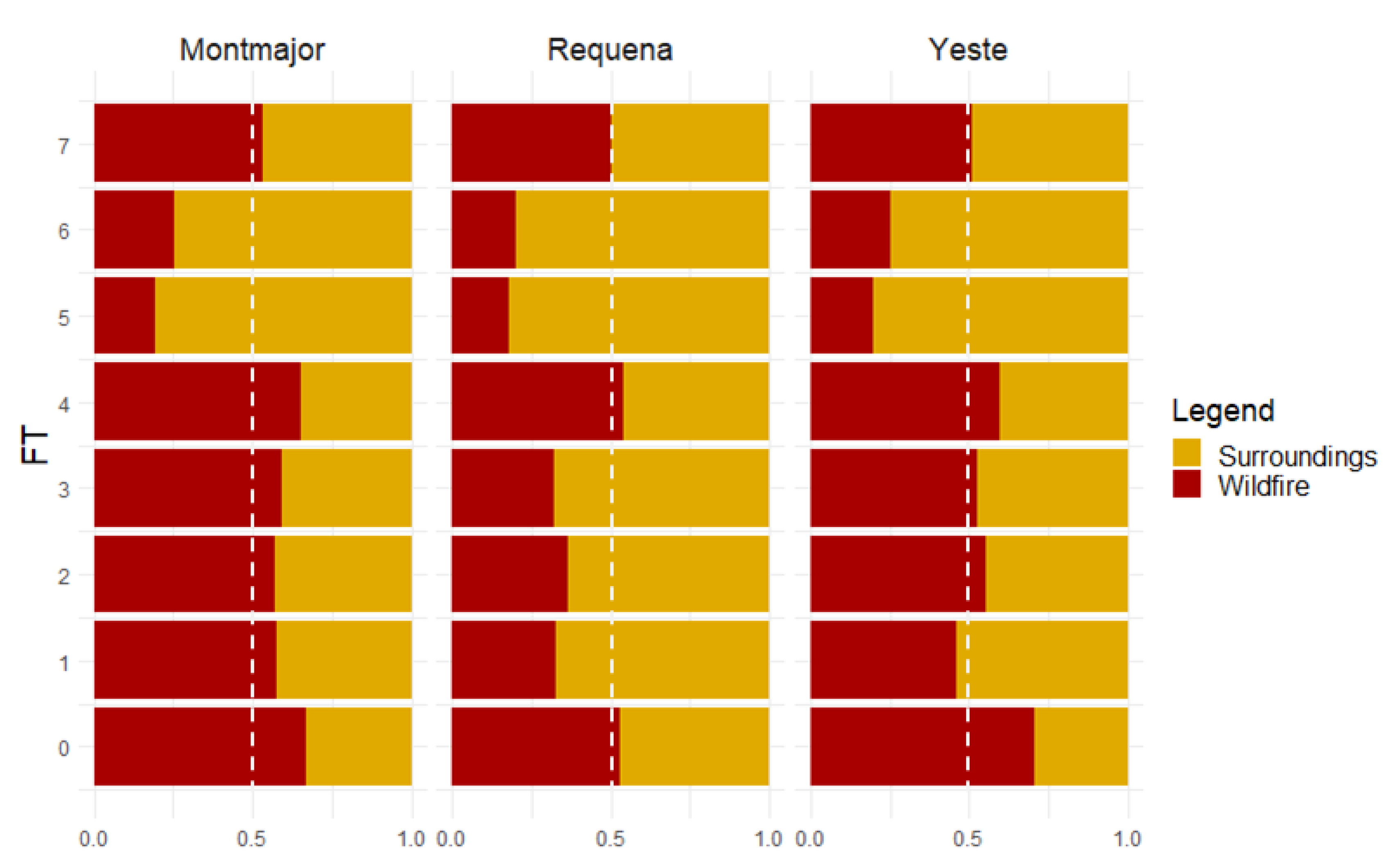
The mapping of fuel type within areas previously affected by wildfires and its comparison with control areas allow determining whether structural differences exists between both forested areas. A review published by Gómez et al. [83] determined, using passive remote sensing data in Spain, that pre-fire vegetation cover was reached after 7–20 years after fire. Rodrigues et al. [55] determined that vegetation recovery time after high-severity wildfires ranges from 21.5 years for high seeding trees, to 25.5 years for resprouter trees and up to 52.9 years for low seeding trees in Spanish Mediterranean forests. Our results are in accordance with Gelabert et al. [64], who pointed out that differences in height, canopy cover and structural diversity indexes were still present after 21 years of a fire in Pinus halepensis forests located within the central sector of the Ebro basin (northeast Spain). Furthermore, though taking into account the moderate accuracy of our models, the mapping results show concordance with our knowledge from field work campaigns. Fuel type 4 in burned areas was mainly related with high stem densities of thin trees in the case of Pinus forests, while Quercus forests where accompanied by bulky shrubs. The presence of fuel types 5 and 6 in burned areas was low, and those burned areas with dominance of tree strata were associated with high presence of shrubs with continuity to tree strata (fuel type 7). Furthermore, the lower presence of fuel types 1, 2 and 3 in Requena burned area may be associated with a high presence of stony areas and climate conditions.

The present study shows the utility of integrating freely available ALS and multispectral data to classify Prometheus fuel type at a regional scale. More research should be done to increase discrimination between fuel type models by integrating other remote sensing datasets. The combination with high-resolution multispectral data or SAR data might improve classification accuracy [28,46]. In this sense, the use of orthophotos with NIR information acquired during recent years within the Spanish context might boost model performance. In addition, further analysis might focus on predicting fuel parameters within areas affected by wildfires as well as analyzing fuel type differences between burned and unburned areas.

5. Conclusions

This study assessed the usefulness of integrating low-point density ALS data and Sentinel 2 data to classify and map Prometheus fuel types in three different topographically complex Mediterranean forests, dominated by pines, oaks and quercus. These areas encompass forests affected by wildfires in 1994 and their surrounding areas. Spearman‘s rank coefficient has been the most powerful selection method to generate a representative and meaningful classification fuel types at regional scale. The SVM with radial kernel method produced the most accurate fuel type classification model, which included three ALS metrics: the 25th percentile of return heights, the percentage of all returns above mean, rumple structural diversity index, and NDVI index from Sentinel 2 images. The classification achieved an overall accuracy of 0.59 after validation. The use of ALS derived diversity structural indices boosts model performance as well as the fusion with multispectral data from Sentinel 2, allowing mapping at 10 m resolution. Forest fuel mapping provides valuable information to assist forest management. The structural characterization of forested areas affected by wildfires after two and a half decades constitutes a relevant input for analyzing post-fire forest treatments as well as to define actions to reduce fuel density at canopy level or lower strata.

References

1. Pausas, J.G.; Llovet, J.; Rodrigo, A.; Vallejo, R. Are wildfires a disaster in the Mediterranean basin?—A review. Int. J. Wildl. Fire 2008, 17, 713–723. [Google Scholar] [CrossRef]
2. Cochrane, M.A.; Schulze, M.D. Fire as a Recurrent Event in Tropical Forests of the Eastern Amazon: Effects on Forest Structure, Biomass, and Species Composition1. Biotropica 1999, 31, 2–16. [Google Scholar] [CrossRef]
3. Oliveira, S.; Oehler, F.; San-Miguel-Ayanz, J.; Camia, A.; Pereira, J.M.C. Modeling spatial patterns of fire occurrence in Mediterranean Europe using Multiple Regression and Random Forest. For. Ecol. Manag. 2012, 275, 117–129. [Google Scholar] [CrossRef]
4. San-Miguel-Ayanz, J.; Rodrigues, M.; de Oliveira, S.S.; Pacheco, C.K.; Moreira, F.; Duguy, B.; Camia, A. Land Cover Change and Fire Regime in the European Mediterranean Region; Springer: Berlin, Germany, 2012; pp. 21–43. [Google Scholar]
5. Estadísticas de Incendios Forestales. Available online: https://www.mapa.gob.es/es/desarrollo-rural/estadisticas/Incendios_default.aspx (accessed on 25 September 2020).
6. Jiménez-Ruano, A.; de la Riva Fernández, J.; Rodrigues, M. Fire regime dynamics in mainland Spain. Part 2: A near-future prospective of fire activity. Sci. Total Environ. 2020, 705, 135842. [Google Scholar] [CrossRef]
7. Mutlu, M.; Popescu, S.C.; Zhao, K. Sensitivity analysis of fire behavior modeling with LIDAR-derived surface fuel maps. For. Ecol. Manag. 2008, 256, 289–294. [Google Scholar] [CrossRef]
8. Mutlu, M.; Popescu, S.C.; Stripling, C.; Spencer, T. Mapping surface fuel models using lidar and multispectral data fusion for fire behavior. Remote Sens. Environ. 2008, 112, 274–285. [Google Scholar] [CrossRef]
9. Chuvieco, E.; Congalton, R.G. Application of remote sensing and geographic information systems to forest fire hazard mapping. Remote Sens. Environ. 1989, 29, 147–159. [Google Scholar] [CrossRef]
10. Ferraz, A.; Bretar, F.; Jacquemoud, S.; Gonçalves, G. The Role of Lidar Systems in Fuel Mapping; INESC: Coimbra, Portugal, 2009; ISSN 1645-2631. [Google Scholar]
11. Merrill, D.F.; Alexander, M.E. Glossary of Forest Fire Management Terms; Canadian Committee on Forest Fire Management, National Research Council of Canada: Ottawa, ON, Canada, 1987. [Google Scholar]
12. Huesca, M.; Riaño, D.; Ustin, S.L. Spectral mapping methods applied to LiDAR data: Application to fuel type mapping. Int. J. Appl. Earth Obs. Geoinf. 2019, 74, 159–168. [Google Scholar] [CrossRef] [Green Version]
13. Anderson, H.E. Aids to Determining Fuel Models for Estimating Fire Behavior; Gen. Tech. Rep. INT-122; U.S. Department of Agriculture, Forest Service, Intermountain Forest and Range Experiment Station: Ogden, UT, USA, 1982; 92p. [CrossRef] [Green Version]
14. Sandberg, D.V.; Ottmar, R.D.; Cushon, G.H. Characterizing fuels in the 21st Century. Int. J. Wildl. Fire 2001, 10, 381–387. [Google Scholar] [CrossRef]
15. Albini, F.A. Estimating Wildfire Behavior and Effects; Gen. Tech. Rep. Int-Gtr-30; U.S. Department of Agriculture, Forest Service, Intermountain Forest and Range Experiment Station: Ogden, UT, USA, 1976; Volume 30.
16. Taylor, S.W.; Alexander, M.E. Field Guide to the Canadian Forest Fire Behavior Prediction (FBP) System, 2nd ed.; B.C. Ministry of Forests and Northern Forestry Centre: Victoria, BC, Canada, 1996. [Google Scholar] [CrossRef]
17. Prometheus, S.V. Management Techniques for Optimization of Suppression and Minimization of Wildfire Effects. System Validation; European Commission: Brussels, Belgium, 2000. [Google Scholar]
18. Arroyo, L.A.; Pascual, C.; Manzanera, J.A. Fire models and methods to map fuel types: The role of remote sensing. For. Ecol. Manag. 2008, 256, 1239–1252. [Google Scholar] [CrossRef] [Green Version]
19. Riaño, D.; Chuvieco, E.; Salas, J.; Palacios-Orueta, A.; Bastarrika, A. Generation of fuel type maps from Landsat TM images and ancillary data in Mediterranean ecosystems. Can. J. Res. 2002, 32, 1301–1315. [Google Scholar] [CrossRef]
20. Chuvieco, E.; Riaño, D.; Van Wagtendok, J.; Morsdof, F. Fuel Loads and Fuel Type Mapping; World Scientific: Singapore, 2003; pp. 119–142. [Google Scholar] [CrossRef]
21. Lasaponara, R.; Lanorte, A. Remotely sensed characterization of forest fuel types by using satellite ASTER data. Int. J. Appl. Earth Obs. Geoinf. 2007, 9, 225–234. [Google Scholar] [CrossRef]
22. Van Wagtendonk, J.W.; Root, R.R. The use of multi-temporal landsat normalized difference vegetation index (NDVI) data for mapping fuel models in Yosemite National Park, USA. Int. J. Remote Sens. 2003, 24, 1639–1651. [Google Scholar] [CrossRef]
23. Arellano-Pérez, S.; Castedo-Dorado, F.; López-Sánchez, C.; González-Ferreiro, E.; Yang, Z.; Díaz-Varela, R.; Álvarez-González, J.; Vega, J.; Ruiz-González, A. Potential of Sentinel-2A Data to Model Surface and Canopy Fuel Characteristics in Relation to Crown Fire Hazard. Remote Sens. 2018, 10, 1645. [Google Scholar] [CrossRef] [Green Version]
24. Lasaponara, R.; Lanorte, A.; Pignatti, S. Characterization and mapping of fuel types for the Mediterranean ecosystems of Pollino National Park in southern Italy by using hyperspectral MIVIS data. Earth Interact. 2006, 10, 1–11. [Google Scholar] [CrossRef]
25. Jia, G.J.; Burke, I.C.; Goetz, A.F.H.; Kaufmann, M.R.; Kindel, B.C. Assessing spatial patterns of forest fuel using AVIRIS data. Remote Sens. Environ. 2006, 102, 318–327. [Google Scholar] [CrossRef]
26. Saatchi, S.; Halligan, K.; Despain, D.G.; Crabtree, R.L. Estimation of Forest Fuel Load From Radar Remote Sensing. IEEE Trans. Geosci. Remote Sens. 2007, 45, 1726–1740. [Google Scholar] [CrossRef]
27. Tanase, M.A.; Panciera, R.; Lowell, K.; Aponte, C. Monitoring live fuel moisture in semiarid environments using L-band radar data. Int. J. Wildl. Fire 2015, 24, 560. [Google Scholar] [CrossRef]
28. Erdody, T.L.; Moskal, L.M. Fusion of LiDAR and imagery for estimating forest canopy fuels. Remote Sens. Environ. 2010, 114, 725–737. [Google Scholar] [CrossRef]
29. García, M.; Riaño, D.; Chuvieco, E.; Salas, J.; Danson, F.M. Multispectral and LiDAR data fusion for fuel type mapping using Support Vector Machine and decision rules. Remote Sens. Environ. 2011, 115, 1369–1379. [Google Scholar] [CrossRef]
30. Andersen, H.-E.; McGaughey, R.J.; Reutebuch, S.E. Estimating forest canopy fuel parameters using LIDAR data. Remote Sens. Environ. 2005, 94, 441–449. [Google Scholar] [CrossRef]
31. González-Ferreiro, E.; Arellano-Pérez, S.; Castedo-Dorado, F.; Hevia, A.; Vega, J.A.; Vega-Nieva, D.; Álvarez-González, J.G.; Ruiz-González, A.D. Modelling the vertical distribution of canopy fuel load using national forest inventory and low-density airbone laser scanning data. PLoS ONE 2017, 12, e0176114. [Google Scholar] [CrossRef]
32. González-Ferreiro, E.; Diéguez-Aranda, U.; Crecente-Campo, F.; Barreiro-Fernández, L.; Miranda, D.; Castedo-Dorado, F. Modelling canopy fuel variables for Pinus radiata D. Don in NW Spain with low-density LiDAR data. Int. J. Wildl. Fire 2014, 23, 350. [Google Scholar] [CrossRef]
33. Hevia, A.; Álvarez-González, J.G.; Ruiz-Fernández, E.; Prendes, C.; Ruiz-González, A.D.; Majada, J.; González-Ferreiro, E. Estimación de variables de combustible de copa y de masa, caracterizando el efecto de las claras en su estructura usando LiDAR aerotransportado. Rev. Teledetec. 2016, 2016, 41–45. [Google Scholar] [CrossRef] [Green Version]
34. Chen, Y.; Zhu, X.; Yebra, M.; Harris, S.; Tapper, N. Development of a predictive model for estimating forest surface fuel load in Australian eucalypt forests with LiDAR data. Environ. Model. Softw. 2017, 97, 61–71. [Google Scholar] [CrossRef]
35. Bright, B.; Hudak, A.; Meddens, A.; Hawbaker, T.; Briggs, J.; Kennedy, R.; Bright, B.C.; Hudak, A.T.; Meddens, A.J.H.; Hawbaker, T.J.; et al. Prediction of Forest Canopy and Surface Fuels from Lidar and Satellite Time Series Data in a Bark Beetle-Affected Forest. Forests 2017, 8, 322. [Google Scholar] [CrossRef] [Green Version]
36. Crespo-Peremarch, P.; Ruiz, L.A.; Balaguer-Beser, A. A comparative study of regression methods to predict forest structure and canopy fuel variables from LiDAR full-waveform data. Rev. Teledetec. 2016, 45, 27. [Google Scholar] [CrossRef] [Green Version]
37. Price, O.F.; Gordon, C.E. The potential for LiDAR technology to map fire fuel hazard over large areas of Australian forest. J. Environ. Manag. 2016, 181, 663–673. [Google Scholar] [CrossRef]
38. Hermosilla, T.; Ruiz, L.A.; Kazakova, A.N.; Coops, N.C.; Moskal, L.M. Estimation of forest structure and canopy fuel parameters from small-footprint full-waveform LiDAR data. Int. J. Wildl. Fire 2014, 23, 224. [Google Scholar] [CrossRef] [Green Version]
39. Romero Ramirez, F.J.; Navarro-Cerrillo, R.M.; Varo-Martínez, M.Á.; Quero, J.L.; Doerr, S.; Hernández-Clemente, R. Determination of forest fuels characteristics in mortality-affected Pinus forests using integrated hyperspectral and ALS data. Int. J. Appl. Earth Obs. Geoinf. 2018, 68, 157–167. [Google Scholar] [CrossRef] [Green Version]
40. García, M.; Saatchi, S.; Casas, A.; Koltunov, A.; Ustin, S.; Ramirez, C.; Balzter, H.; García, M.; Saatchi, S.; Casas, A.; et al. Extrapolating Forest Canopy Fuel Properties in the California Rim Fire by Combining Airborne LiDAR and Landsat OLI Data. Remote Sens. 2017, 9, 394. [Google Scholar] [CrossRef] [Green Version]
41. Botequim, B.; Fernandes, P.M.; Borges, J.G.; González-Ferreiro, E.; Guerra-Hernández, J. Improving silvicultural practices for Mediterranean forests through fire behaviour modelling using LiDAR-derived canopy fuel characteristics. Int. J. Wildl. Fire 2019, 28, 823. [Google Scholar] [CrossRef]
42. Sánchez Sánchez, Y.; Martínez-Graña, A.; Santos Francés, F.; Mateos Picado, M. Mapping wildfire ignition probability using sentinel 2 and LiDAR (Jerte Valley, Cáceres, Spain). Sensors 2018, 18, 826. [Google Scholar] [CrossRef] [Green Version]
43. López-Serrano, P.M.; López-Sánchez, C.A.; Alvarez-González, J.G.; García-Gutiérrez, J. A Comparison of Machine Learning Techniques Applied to Landsat-5 TM Spectral Data for Biomass Estimation. Can. J. Remote Sens. 2016, 42, 690–705. [Google Scholar] [CrossRef]
44. Alonso-Benito, A.; Arroyo, L.; Arbelo, M.; Hernández-Leal, P.; Alonso-Benito, A.; Arroyo, L.A.; Arbelo, M.; Hernández-Leal, P. Fusion of WorldView-2 and LiDAR Data to Map Fuel Types in the Canary Islands. Remote Sens. 2016, 8, 669. [Google Scholar] [CrossRef] [Green Version]
45. Chirici, G.; Scotti, R.; Montaghi, A.; Barbati, A.; Cartisano, R.; Lopez, G.; Marchetti, M.; Mcroberts, R.E.; Olsson, H.; Corona, P. Stochastic gradient boosting classification trees for forest fuel types mapping through airborne laser scanning and IRS LISS-III imagery. Int. J. Appl. Earth Obs. Geoinf. 2013, 25, 87–97. [Google Scholar] [CrossRef] [Green Version]
46. Marino, E.; Ranz, P.; Tomé, J.L.; Noriega, M.Á.; Esteban, J.; Madrigal, J. Generation of high-resolution fuel model maps from discrete airborne laser scanner and Landsat-8 OLI: A low-cost and highly updated methodology for large areas. Remote Sens. Environ. 2016, 187, 267–280. [Google Scholar] [CrossRef]
47. Montealegre, A.L.; Lamelas, M.T.; García-Martín, A.; de la Riva, J.; Escribano, F. Cartografía de Modelos de Combustible Mediante Combinación de Imágenes LiDAR, SAR y Ópticas en el Centro de Adiestramiento “San Gregorio”. In III Congreso Nacional de i+d en Defensa y Seguridad; Asorey, R., Devesa, R., Solla, M.M., Pousada, J.M., Eds.; University of Vigo: Vigo, Spain, 2015; pp. 1185–1192. ISBN 978-84-944537-0-0. [Google Scholar]
48. Kane, V.R.; Bakker, J.D.; McGaughey, R.J.; Lutz, J.A.; Gersonde, R.F.; Franklin, J.F. Examining conifer canopy structural complexity across forest ages and elevations with LiDAR data. Can. J. Res. 2010, 40, 774–787. [Google Scholar] [CrossRef]
49. Listopad, C.M.C.S.; Masters, R.E.; Drake, J.; Weishampel, J.; Branquinho, C. Structural diversity indices based on airborne LiDAR as ecological indicators for managing highly dynamic landscapes. Ecol. Indic. 2015, 57, 268–279. [Google Scholar] [CrossRef]
50. Stefanidou, A.; Gitas, I.Z.; Katagis, T. A national fuel type mapping method improvement using sentinel-2 satellite data. Geocarto Int. 2020, 1–21. [Google Scholar] [CrossRef]
51. De Santis, A.; Chuvieco, E. GeoCBI: A modified version of the Composite Burn Index for the initial assessment of the short-term burn severity from remotely sensed data. Remote Sens. Environ. 2009, 113, 554–562. [Google Scholar] [CrossRef]
52. Martínez, S.; Chuvieco, E.; Aguado, I.; Salas, J. Severidad y regeneración en grandes incendios forestales: Análisis a partir de series temporales de imágenes landsat. Rev. Teledetec. 2017, 2017, 17–32. [Google Scholar] [CrossRef] [Green Version]
53. Viana-Soto, A.; Aguado, I.; Martínez, S. Assessment of Post-Fire Vegetation Recovery Using Fire Severity and Geographical Data in the Mediterranean Region (Spain). Environments 2017, 4, 90. [Google Scholar] [CrossRef] [Green Version]
54. De Santis, A.; Chuvieco, E. Burn severity estimation from remotely sensed data: Performance of simulation versus empirical models. Remote Sens. Environ. 2007, 108, 422–435. [Google Scholar] [CrossRef]
55. Rodrigues, M.; Ibarra, P.; Echeverría, M.; Pérez-Cabello, F.; de la Riva, J. A method for regional-scale assessment of vegetation recovery time after high-severity wildfires. Prog. Phys. Geogr. Earth Environ. 2014, 38, 556–575. [Google Scholar] [CrossRef]
56. Evans, J.S.; Hudak, A.T. A Multiscale Curvature Algorithm for Classifying Discrete Return LiDAR in Forested Environments. IEEE Trans. Geosci. Remote Sens. 2007, 45, 1029–1038. [Google Scholar] [CrossRef]
57. Montealegre, A.L.; Lamelas, M.T.; de la Riva, J. A Comparison of Open-Source LiDAR Filtering Algorithms in a Mediterranean Forest Environment. IEEE J. Sel. Top. Appl. Earth Obs. Remote Sens. 2015, 8, 4072–4085. [Google Scholar] [CrossRef] [Green Version]
58. Renslow, M. Manual of Airborne Topographic Lidar; The American Society for Photogrammetry and Remote Sensing: Bethesda, MD, USA, 2013; ISBN 978-1570830976. [Google Scholar]
59. Montealegre, A.; Lamelas, M.; Riva, J. Interpolation Routines Assessment in ALS-Derived Digital Elevation Models for Forestry Applications. Remote Sens. 2015, 7, 8631–8654. [Google Scholar] [CrossRef] [Green Version]
60. McGaughey, R. FUSION/LDV: Software for LIDAR Data Analysis and Visualization 2009. V3.10; USDA Forest Service: Washington, DC, USA, 2014; pp. 1–212.
61. Næsset, E. Practical large-scale forest stand inventory using a small-footprint airborne scanning laser. Scand. J. Res. 2004, 19, 164–179. [Google Scholar] [CrossRef]
62. Lesak, A.A.; Radeloff, V.C.; Hawbaker, T.J.; Pidgeon, A.M.; Gobakken, T.; Contrucci, K. Modeling forest songbird species richness using LiDAR-derived measures of forest structure. Remote Sens. Environ. 2011, 115, 2823–2835. [Google Scholar] [CrossRef]
63. Weisberg, P.J.; Dilts, T.E.; Becker, M.E.; Young, J.S.; Wong-Kone, D.C.; Newton, W.E.; Ammon, E.M. Guild-specific responses of avian species richness to LiDAR-derived habitat heterogeneity. Acta Oecologica 2014, 59, 72–83. [Google Scholar] [CrossRef]
64. Gelabert, P.J.; Montealegre, A.L.; Lamelas, M.T.; Domingo, D. Forest structural diversity characterization in Mediterranean landscapes affected by fires using Airborne Laser Scanning data. Gisci. Remote Sens. 2020, 57, 497–509. [Google Scholar] [CrossRef]
65. Rouse, J.W.; Haas, R.H.; Shell, J.A.; Deering, D.W. Monitoring vegetation systems in the Great Plains with ERTS. In Proceedings of the Third Earth Resources Technology Satellite-1Symposium, Washington, DC, USA, 10–14 December 1973; NASA Scientific and Technical Information Office: Washington, DC, USA, 1974; Volume 1, pp. 309–317. [Google Scholar]
66. Hunt, E.R.; Rock, B.N. Detection of changes in leaf water content using Near- and Middle-Infrared reflectances. Remote Sens. Environ. 1989, 30, 43–54. [Google Scholar] [CrossRef]
67. Gao, B.C. NDWI—A normalized difference water index for remote sensing of vegetation liquid water from space. Remote Sens. Environ. 1996, 58, 257–266. [Google Scholar] [CrossRef]
68. Xu, H. Modification of normalised difference water index (NDWI) to enhance open water features in remotely sensed imagery. Int. J. Remote Sens. 2006, 27, 3025–3033. [Google Scholar] [CrossRef]
69. Key, C.H.; Benson, N. Landscape Assessment: Ground Measure of Severity, the Composite Burn Index; and remote sensing of severity, the normalized burn ratio. In FIREMON: Fire Effects Monitoring and Inventory System; Lutes, D.C., Keane, R.E., Caratti, J.F., Key, C.H., Benson, N.C., Gangi, L.J., Eds.; Gen. Tech. Rep. RMRS-GTR-164; USDA Forest Service, Rocky Mountain Research Station: Ogden, UT, USA, 2005. [Google Scholar]
70. Kauth, R.; Thomas, G.S. The Tasselled Cap—A Graphic Description of the Spectral-Temporal Development of Agricultural Crops as Seen by Landsat; Purdue University: West Lafayette, IN, USA, 1976. [Google Scholar]
71. Domingo, D.; Lamelas, M.T.; Montealegre, A.L.; García-Martín, A.; de la Riva, J. Estimation of total biomass in Aleppo pine forest stands applying parametric and nonparametric methods to low-density airborne laser scanning data. Forests 2018, 9, 158. [Google Scholar] [CrossRef] [Green Version]
72. Rodrigues, M.; De la Riva, J. An insight into machine-learning algorithms to model human-caused wildfire occurrence. Environ. Model. Softw. 2014, 57, 192–201. [Google Scholar] [CrossRef]
73. Liaw, A.; Wiener, M. Classification and Regression by randomForest. R News 2002, 2, 18–22. [Google Scholar]
74. Van Essen, D.C.; Drury, H.A.; Dickson, J.; Harwell, J.; Hanlon, D.; Anderson, C.H. An integrated software suite for surface-based analyses of cerebral cortex. J. Am. Med. Inform. Assoc. 2001, 8, 443–459. [Google Scholar] [CrossRef] [PubMed] [Green Version]
75. García-Gutiérrez, J.; Martínez-Álvarez, F.; Troncoso, A.; Riquelme, J.C. A comparison of machine learning regression techniques for LiDAR-derived estimation of forest variables. Neurocomputing 2015, 167, 24–31. [Google Scholar] [CrossRef]
76. Foody, G.M. Explaining the unsuitability of the kappa coefficient in the assessment and comparison of the accuracy of thematic maps obtained by image classification. Remote Sens. Environ. 2020, 239, 111630. [Google Scholar] [CrossRef]
77. Kristensen, T.; Næsset, E.; Ohlson, M.; Bolstad, P.V.; Kolka, R. Mapping Above- and Below-Ground Carbon Pools in Boreal Forests: The Case for Airborne Lidar. PLoS ONE 2015, 10, e0138450. [Google Scholar] [CrossRef] [PubMed] [Green Version]
78. Domingo, D.; Alonso, R.; Lamelas, M.T.; Montealegre, A.L.; Rodríguez, F.; de la Riva, J. Temporal transferability of pine forest attributes modeling using low-density airborne laser scanning data. Remote Sens. 2019, 11, 261. [Google Scholar] [CrossRef] [Green Version]
79. Hu, Y.; Xu, X.; Wu, F.; Sun, Z.; Xia, H.; Meng, Q.; Huang, W.; Zhou, H.; Gao, J.; Li, W.; et al. Estimating forest stock volume in Hunan Province, China, by integrating in situ plot data, Sentinel-2 images, and linear and machine learning regression models. Remote Sens. 2020, 12, 186. [Google Scholar] [CrossRef] [Green Version]
80. Domingo, D.; Montealegre, A.L.; Lamelas, M.T.; García-Martín, A.; de la Riva, J.; Rodríguez, F.; Alonso, R. Quantifying forest residual biomass in Pinus halepensis Miller stands using Airborne Laser Scanning data. Gisci. Remote Sens. 2019, 56, 1210–1232. [Google Scholar] [CrossRef]
81. Janitza, S.; Hornung, R. On the overestimation of random forest’s out-of-bag error. PLoS ONE 2018, 13, e0201904. [Google Scholar] [CrossRef]
82. Alonso-Benito, A.; Arbelo, M.; Hernández-Leal, P. Tipos de Combustibles Con Datos LiDAR de Baja Densidad. In Teledetección: Humedales y Espacios Protegidos. XVI Congreso de la Asociación Española de Teledetección, Seville, Spain, 21–23 October 2015; Asociación Española de Teledetección: Sevilla, Spain, 2015. [Google Scholar]
83. Gómez, C.; Alejandro, P.; Hermosilla, T.; Montes, F.; Pascual, C.; Ruiz, L.Á.; Álvarez-Taboada, F.; Tanase, M.A.; Valbuena, R. Remote sensing for the Spanish forests in the 21st century: A review of advances, needs, and opportunities. For. Syst. 2019, 28, 2171–9292. [Google Scholar] [CrossRef]
Figure 1. Study area with the location of areas affected by wildfires, surrounding areas, field plots and pre-fire vegetation.
Remotesensing 12 03660 g001
Figure 2. Relative presence of fuel types for the different forested areas under study. The value 0 refers to bare soil, and the values 1 to 7 stands for the Prometheus fuel types.
Remotesensing 12 03660 g002
Figure 3. Fuel type classification mapping using SVM with radial kernel within the forested areas under study.
Remotesensing 12 03660 g003
Figure 4. Relative presence, expressed between 0 and 1, of fuel types in areas affected by the three wildfires or their surroundings.
Remotesensing 12 03660 g004