Article

Suppression of Wind Ripples and Microwave Backscattering Due to Turbulence Generated by Breaking Surface Waves

by
Stanislav A. Ermakov
1,2,3,*,
Vladimir A. Dobrokhotov
1,
Irina A. Sergievskaya
1,2 and
Ivan A. Kapustin
1,2
1
Institute of Applied Physics, Russian Academy of Sciences, 46 Uljanova St., 603950 Nizhny Novgorod, Russia
2
Radiophysics Department, Lobachevsky State University of Nizhny Novgorod, 23 Gagarin Av., 603950 Nizhny Novgorod, Russia
3
Department of Shipbuilding, Hydraulic Engineering and Environmental Protection, Volga State University of Water Transport, 5 Nesterova St., 603950 Nizhny Novgorod, Russia
*
Author to whom correspondence should be addressed.
Remote Sens. 2020, 12(21), 3618; https://doi.org/10.3390/rs12213618
Submission received: 3 October 2020 / Revised: 2 November 2020 / Accepted: 3 November 2020 / Published: 5 November 2020

Abstract

:
The role of wave breaking in microwave backscattering from the sea surface is a problem of great importance for the development of theories and methods on ocean remote sensing, in particular for oil spill remote sensing. Recently it has been shown that microwave radar return is determined by both Bragg and non-Bragg (non-polarized) scattering mechanisms and some evidence has been given that the latter is associated with wave breaking, in particular, with strong breaking such as spilling or plunging. However, our understanding of mechanisms of the action of strong wave breaking on small-scale wind waves (ripples) and thus on the radar return is still insufficient. In this paper an effect of suppression of radar backscattering after strong wave breaking has been revealed experimentally and has been attributed to the wind ripple suppression due to turbulence generated by strong wave breaking. The experiments were carried out in a wind wave tank where a frequency modulated wave train of intense meter-decimeter-scale surface waves was generated by a mechanical wave maker. The wave train was compressed according to the gravity wave dispersion relation (“dispersive focusing”) into a short-wave packet at a given distance from the wave maker. Strong wave breaking with wave crest overturning (spilling) occurred for one or two highest waves in the packet. Short decimeter-centimeter-scale wind waves were generated at gentle winds, simultaneously with the long breaking waves. A Ka-band scatterometer was used to study microwave backscattering from the surface waves in the tank. The scatterometer looking at the area of wave breaking was mounted over the tank at a height of about 1 m above the mean water level, the incidence angle of the microwave radiation was about 50 degrees. It has been obtained that the radar return in the presence of short wind waves is characterized by the radar Doppler spectrum with a peak roughly centered in the vicinity of Bragg wave frequencies. The radar return was strongly enhanced in a wide frequency range of the radar Doppler spectrum when a packet of long breaking waves arrived at the area irradiated by the radar. After the passage of breaking waves, the radar return strongly dropped and then slowly recovered to the initial level. Measurements of velocities in the upper water layer have confirmed that the attenuation of radar backscattering after wave breaking is due to suppression of short wind waves by turbulence generated in the breaking zone. A physical analysis of the effect has been presented.

Graphical Abstract

1. Introduction

At the present time a lot of studies are focusing on a better understanding of microwave scattering from the sea surface. The increased interest in the problem is associated with new features of microwave backscattering revealed in field experiments and related to breaking waves, in particular in experiments on microwave radar probing of oil slicks. It has been demonstrated, amongst others, that the widely used two-scale Bragg theory [1,2] is unable to describe some features of microwave scattering when interpreting observations with co-polarized radar both for clean water surface and for oil slicks (see, e.g., [3,4,5]). It was obtained, in particular, that a significant inconsistency between the theory and experiment occurs for the polarization ratio, that is the ratio of the radar backscatter at vertical and horizontal polarizations. A lack of understanding of microwave scattering has been found regarding effects of wave breaking, either strong or micro breaking at low—to-moderate wind velocities. Strong wave breaking (spilling or plunging) is characterized by wave crest overturning (see, e.g., [6,7,8]) and is typical for meter (m)-scale waves. Micro breaking occurs for centimeter-decimeter (cm-dm)-scale waves and is associated with generation of small-scale structures—parasitic ripples, toes and bulges near the wave crests [8,9,10]. Both types of wave breaking are supposed to be responsible for particularities of microwave scattering from the sea surface, although their relative role is still not well understood, in particular, when interpreting radar observations of oil slicks [11,12,13]. The role of small-scale nonlinear structures on the profile of short Gravity–Capillary Waves (GCW), often characterized as bound waves, in microwave scattering has been extensively studied in a number of wave tank experiments (see, e.g., [14,15,16,17,18,19]). It was obtained when analyzing radar Doppler spectra that the velocities of microwave scatterers can differ from the intrinsic velocities of linear free GCW with Bragg wavelengths and the scatterers can be associated with the nonlinear structures moving with the phase velocities of carrying cm-dm-scale waves [15,18,20]. Correspondingly, radar Doppler spectra can be bimodal [17,18,21] thus indicating two types of microwave scatterers—free Bragg waves and bound waves. It was shown that bimodal Dopper spectrum can appear for an upwind look direction, while for downwind observations there was typically only one-peak spectrum for free waves. This conclusion is consistent with the result [19] that the radar return maximum occurs near the “toe” of a breaking wave and that bound waves are mostly located on the forward slopes of dm-scale waves. Plant et.al. [17] hypothesized that “turbulence associated with bound waves” suppresses free wind waves and the areas where bound or free waves dominate are separated on the water surface. In general, the microwave sea clutter can be considered as a result of different types of scattering: Bragg scattering, and non-polarized scattering—burst scattering from the crests of waves just before they break and whitecap scattering [22].
A wave breaking strongly also affects radar return at strong winds. It was previously obtained that microwave radar backscattering from the sea surface at very high wind conditions is characterized by a tendency to saturate the Normalized Radar Cross Section (NRCS) as a function of wind speed and even an NRCS decrease [23,24,25]. This demonstrates that the effective roughness of the sea surface in the presence of intense wave breaking does not grow monotonically with wind and some physical processes in the vicinity of the ocean–atmosphere interface can limit the wind wave growth. Sea sprays attenuating the incident and reflected microwaves, sea foam changing the air–sea interaction as well as the microwave reflection coefficients and air bubbles transporting surfactants to the sea surface from the subsurface water can be, amongst others, responsible for the effect of saturation or reduction of radar backscattering. Everyday visual observations also indicate that the sea surface looks smoother behind wave breaking crests.
The breaking of wave crests and the formation of spilling breakers (see, e.g., [7,8,26,27] and references therein) significantly contributes to the wind wave dynamics. It has been shown experimentally (see, e.g., [26,27]) that a coherent vortex and turbulence are generated in the upper water layer after wave crest overturning. The vortex induces a non-uniform surface current which, according to [27,28], can lead to wind wave amplification and even wave blocking, while turbulence generated by wave breakers results obviously in suppression of small-scale wind waves.
Suppression of small-scale wind waves due to turbulence is particularly important in the context of the problem of remote sensing of oil slicks. This is because the areas of damping of wind waves appear in radar imagery as areas of low backscatter which can be mistakenly supposed to be surfactant slicks or oil spills. Apart from the enhanced wave suppression due to turbulence generated by wave breakers the latter also produce a huge amount of air bubbles in the upper water layer. The bubbles accumulate surfactants dissolved in water and transport them to the water surface resulting in surfactant accumulation and additional wave damping. So, investigations of the action of wave breaking on small-scale wind waves and on microwave scattering are very important when studying the problem of oil slick remote sensing.
Wave damping due to turbulence was studied in a number of papers (see, e.g., [28,29,30,31,32,33] and references therein). It has been shown in [33] that the damping can be described in the frame of semi empirical theory of turbulence in terms of an eddy viscosity. The latter, as shown in [33], demonstrates a sort of resonance growth when the integral scale of turbulent eddies is comparable in size with wavelengths.
In this paper we report on a new effect of Ka-band radar backscatter reduction after the passage of a packet of meter-decimeter-scale strongly breaking waves. We have not found similar effects described in the literature before. The only one closest to the considered problem is a hypothesis of Plant et al. [17], according to which turbulence associated with bound waves can suppress freely propagating surface waves, but this hypothesis was not supported by measurements. It is shown below that the backscatter reduction is associated with suppression of centimeter–millimeter (mm)-scale waves by turbulence generated due to strong wave breaking. The effect of surfactant transport by bubbles, mentioned above, is not considered here and will be studied elsewhere.
The paper is organized as follows. Section 2 describes an experimental setup, as well as methodologies of generation of m-scale breaking waves and small-scale wind waves, of surface wave measurements with wire gauges and of microwave backscattering with a Ka-band scatterometer. A multi sensor methodology for the investigation of turbulence due to wave breakers using an acoustic Doppler velocimeter (ADV), wire gauges and video recording of trajectories of small surface floats are also described in Section 2. The results of experiments are collected in Section 3 and are discussed in Section 4. Summary results are presented in Section 5.

2. Materials and Methods

Experiments were carried out in the Oval Wind Wave Tank (OWWT) of the Institute of Applied Physics of the Russian Academy of Sciences (see, [34] for more detail). The experimental setup is shown schematically in Figure 1. The cross section of the tank water channel is 30 cm × 30 cm, and the air channel is 30 cm × 30 cm, too. The radius of semicircular sections is about 1.8 m. the length of the middle straight sections is 2.5 m. The wind flow in the tank is produced with a ventilator at controlled rotation speeds. The mean wind velocities in the tank can be varied in a wide range, up to 15 m/s, but in the experiments only wind waves at gentle winds were studied. A beach was mounted at the working part end of the tank to reduce reflected backward propagating long waves.

2.1. Surface Wave Generation and Measurements

Wind waves were generated at low velocities of the air flow in the range from about 0.9 m/s to 2.2 m/s. The water part of the tank was partly locked by a mechanical wave maker mounted at a distance of 2.4 m from the ventilator, thus shortening the wind wave fetch which is in our experiments was about 8.5 m, so only short gravity–capillary wind waves were developed in the tank (see below). The water surface elevations due to waves were measured with wire wave gauges. The gauges measure the conductivity between two parallel vertical wires of about 30 cm in length and 3 mm distance between the wires. The gauge response is practically linear regarding the surface water elevations, even for wave heights up to 5 cm and more. One of the gauges was mounted near the mechanical wave maker, and another one was co-located with the radar footprint (see below).
The mechanical wave maker generated intense, non-breaking, low-frequency (LF) wave trains with a controlled linearly varying frequency. When propagating along the tank the frequency modulated wave train was transformed due to a dispersion wave focusing into a short-wave train. The wave train was compressed at a distance of about 8.5 m from the wave maker and contained one or two individual breaking waves (see Figure 2). The heights of the breaking waves were in the range from 6 cm to 8 cm, and the breaking wave period was about 0.6 s. In the experiments the LF wave propagation direction was the same as for the wind waves.
One can see that strong difference occurs between the packet wavelet spectra in the area of wave generation (Figure 2, bottom left panel) and the area of wave packet compression (Figure 2, bottom right panel).

2.2. Radar Measurements

A Ka-band scatterometer used in our experiments is a coherent system operating in a continuous wave regime and radiating microwave frequencies modulated around the central frequency of 37 GHz (the working wavelength of 8.7 mm). The scatterometer allows one to measure both amplitude and phase of scattered microwaves and thus to analyze the Doppler spectrum of radar return. The scatterometer operates normally at VV (Vertical-Vertical)-polarization, but the measurements in experiment were carried out both at VV- and HH (Horizontal-Horizontal)-polarizations when simply turning the device around its axis. The scatterometer was mounted at a height of about 1 m over the water surface, the incidence angle of microwaves was 55 degrees, the radar look direction was opposite to the wind wave/breaking wave propagation direction. The antenna pattern width is about 5 deg., and the radar footprint was elliptical with the across/along tank axes of about 17.4 and 30 cm, respectively. The radar footprint was co-located with the area of wave breaking. An example of the radar Doppler spectrum for the case of wind waves at VV and HH-polarizations at the wind speed of 1.1 m/s is shown in Figure 3. The spectrum demonstrates a prominent peak for both polarizations in the frequency of about 60 Hz, and the spectrum level and the peak offset are very sensitive to wind velocity (see below for more detail). The low-frequency part of the spectrum at frequencies below 40 Hz is associated with apparatus effects and parasitic reflections from quasi stable objects in laboratory; this part was removed when estimating characteristics of the radar return.

2.3. Complex Measurements of Turbulence Due to Breaking of Surface Waves

A methodology of complex measurements of hydrodynamic turbulence generated by breaking waves was developed and based on acoustic measurements of velocities in the upper water layer, the wire gauge use and a video recording of the movement of surface floats. An ultrasonic Acoustic Doppler Velocimeter “SonTek MICRO ADV” was placed 2.5 cm below the water surface in the area of breaking of LF surface waves. The instrument allowed us to measure three components of flow velocities: vertical, longitudinal (along the wave tank) and transverse (across the tank) velocity components associated with surface waves and with turbulence appeared after wave breaking. Special suspension containing small particles (the size of about 10 micrometer) was added to water in the tank to enhance acoustic scattering and thus to improve reliability of velocity measurements with ADV. The ADV frequency bandwidth is 25 Hz. The wire gauge was used simultaneously with ADV to measure independently the spectrum of surface waves. An example of the ADV spectrum of different velocity components for the case of 1.2 Hz LF waves is shown in Figure 4. The ADV spectra demonstrate a peak at the long wave frequency for longitudinal and vertical components and nearly the noise level for the cross-wind velocity.
Cross-correlation analysis for the vertical and longitudinal velocity components in the frequency range of LF waves gives the phase shift close to π/2 thus indicating that these components correspond to the orbital velocity components of deep-water surface waves. In the case of wave breaking the ADV spectra of longitudinal and vertical velocities contain both wave and turbulent motions which spectra are partly overlapped. The latter makes it difficult to select the spectra of turbulence. However, for plane LF waves propagating along the tank the orbital velocity in the cross-tank direction is absent, and ADV measurements of a transverse velocity component can indicate the presence of non-wave (turbulent) velocity components. To retrieve turbulent velocities, we use the spectra of all three components after removal the wave peaks from the spectra of vertical and longitudinal velocities (see, Section 3).
Video recording of movements of small floats placed on the water surface after wave breaking was used additionally to ADV/wire gauge measurements. This allowed us to retrieve the float trajectories (see Figure 5) when fixing float positions at consecutive frames. The trajectories in Figure 5a for the case of LF breaking waves clearly indicate that loops occur due to turbulent eddies in the upper water layer, while for the case of non-breaking waves the markers oscillate due to wave orbital velocities practically along a straight line (see Figure 5b). Analysis of the float movement gives further proof of the presence of turbulent eddies and one can estimate, at least roughly, their characteristics (see below).

3. Results

3.1. Surface Wave Spectra and Radar Doppler Spectra without Wave Breaking

Let us first consider the spectrum of wind waves propagating in the absence of intense LF waves. The wind wave spectra for the studied range of wind velocities are shown in Figure 6a, and the frequencies of dominant wind waves estimated as “a center of gravity” of the wind wave spectrum are presented in Figure 6b. One can see that the wind wave spectrum maximum varies in the frequency range from about 5 to 3.5 Hz (see Figure 6b). This means that the dominant wind wavelengths are within the range from about 6 to 13 cm, which are at least several times smaller than the wavelengths of mechanically-generated LF breaking waves. Figure 6 also indicates the wave age, defined as the ratio of the dominant wave velocity ( V d ) to the wind speed ( V W ).
Now we turn to the results on the Doppler spectra of radar return for the case of wind waves and breaking waves. The Doppler spectra of radar backscattering at VV-polarization for purely wind waves are depicted in Figure 7a. The Doppler shift found as “a center of gravity” of the Doppler spectrum moves to higher frequencies and its width increases with wind velocity, as shown in Figure 7b.
The spectra at HH-polarization are similar to those in Figure 7, but their level is lower than for VV-polarization indicating that radar return at HH-polarization is smaller than at VV-polarization. Radar Doppler shifts at HH-polarization for the studied wind wave regimes are indistinguishable from the shifts at VV-polarization. Different intensities of backscattering at two polarizations can be characterized by the Polarization Ratio P R = I V V / I H H , where I V V , I H H are the intensities of radar backscattering at VV and HH polarizations, respectively (see Figure 8). The red line in Figure 8 corresponds to theoretical values in the frame of the Bragg theory [1]. One can conclude from Figure 8 that radar backscattering from the background wind waves is neither non polarized (NP) scattering for which P R = 1 nor purely Bragg one, although some PR-values can be rather close to the Bragg theory (see Section 4).

3.2. Effects of Wave Breaking on Wind Waves and Radar Return

The action of wave breaking on short wind waves and on radar backscatter is illustrated in Figure 9. Three different domains can be distinguished clearly in a time series of surface waves and radar backscatter. The first domain corresponds to background small-scale wind waves before the LF wave packet came to the studied area. When the breaking waves enter the radar footprint the backscatter is strongly enhanced. After the intense waves leave the study area the radar return decreases below the initial level thus indicating that the wind waves are suppressed after the passage of breaking waves. After about 10–15 s both the wind wave intensity and the radar backscatter are restored to the initial level.
Spectra of surface waves in the presence of wind waves and long breaking waves during and after the passage of breaking waves (see Figure 10) are strongly different from the case of purely wind waves in Figure 6.
First of all, the spectrum maximum of purely wind waves (Figure 10a) becomes indistinguishable in the breaking zone (Figure 10b) because the spectra of LF breaking waves and of wind waves overlap. After the highest breaking wave passage in the area of greatest suppression of the radar signal a low-intensity LF peak (see Figure 10c) is seen in the spectrum due to weak LF wave remains. The spectrum level in the range of wind wave frequencies is some dBs lower after wave breaking when compared to the case of wind waves before the breaking. Figure 10c, therefore, clearly demonstrates the effect of suppression of wind waves due to LF wave breaking.
Radar Doppler spectra in the presence of wind waves before, during and after the passage of breaking waves are shown in Figure 11a–c. During the passage of breaking waves the backscattering is enhanced in a wide frequency range up to at least 300 Hz (see Figure 11b), the spectrum values within the range from about 50 to 250 Hz are approximately the same as the spectrum maximum at frequencies of 60–80 Hz before breaking waves arrived (cf. Figure 11a,b). The spectrum level in Figure 11b practically does not depend on wind velocity, indicating that the scattering is determined mostly by breaking waves, rather than wind waves. After the breaking waves leave the studied area the Doppler spectrum is reduced (Figure 11c); that is consistent with the wind wave spectrum decrease in Figure 10c.

3.3. Turbulence Generated by Breaking Waves

The results of ADV measurements of velocities in the upper water layer are presented in Figure 12 for the case of breaking LF waves in the presence and in the absence of wind waves.
One can conclude from Figure 12a,b that for the case of “no wind waves” the vertical, longitudinal and transverse velocity components are absent in the ADV signal before LF breaking waves. After the passage of breaking LF waves the spectrum is strongly enhanced at frequencies up to 4 Hz. The spectrum intensity level in this frequency range is roughly the same for the vertical, longitudinal and transverse velocity components at frequencies higher than the frequencies of breaking waves. This part of the ADV spectrum can be attributed to turbulent pulsations generated by wave breakers. The difference between the transverse and two other components is that the spectral peak corresponding to LF breaking waves (see Figure 12a) is not practically seen in the spectrum of transverse velocity. In the presence of wind waves (Figure 12c,d) the velocity spectrum shows a local maximum around 4 Hz for all three components corresponding to wind waves. The frequency of the local maximum of the velocity spectrum is a little higher than the frequency of the dominant wind waves (see Figure 6b). This is because the velocity spectrum is proportional to the wind wave height spectrum multiplied by the squared frequency. After the passage of LF breaking waves the spectrum in the frequency range of wind waves is strongly suppressed as it is seen in Figure 12. This is consistent with the results of the surface elevation measurements with the wire gauge shown in Figure 10.
Turbulent velocities were estimated when integrating the ADV spectra of three velocity components over the low-frequency spectral range (up to frequencies of about 3.5 Hz). The estimation of r.m.s. turbulent velocity gave the value of about 1 cm/s. Similar values of turbulent velocities were obtained estimated independently using video records of surface float movements.

4. Discussion

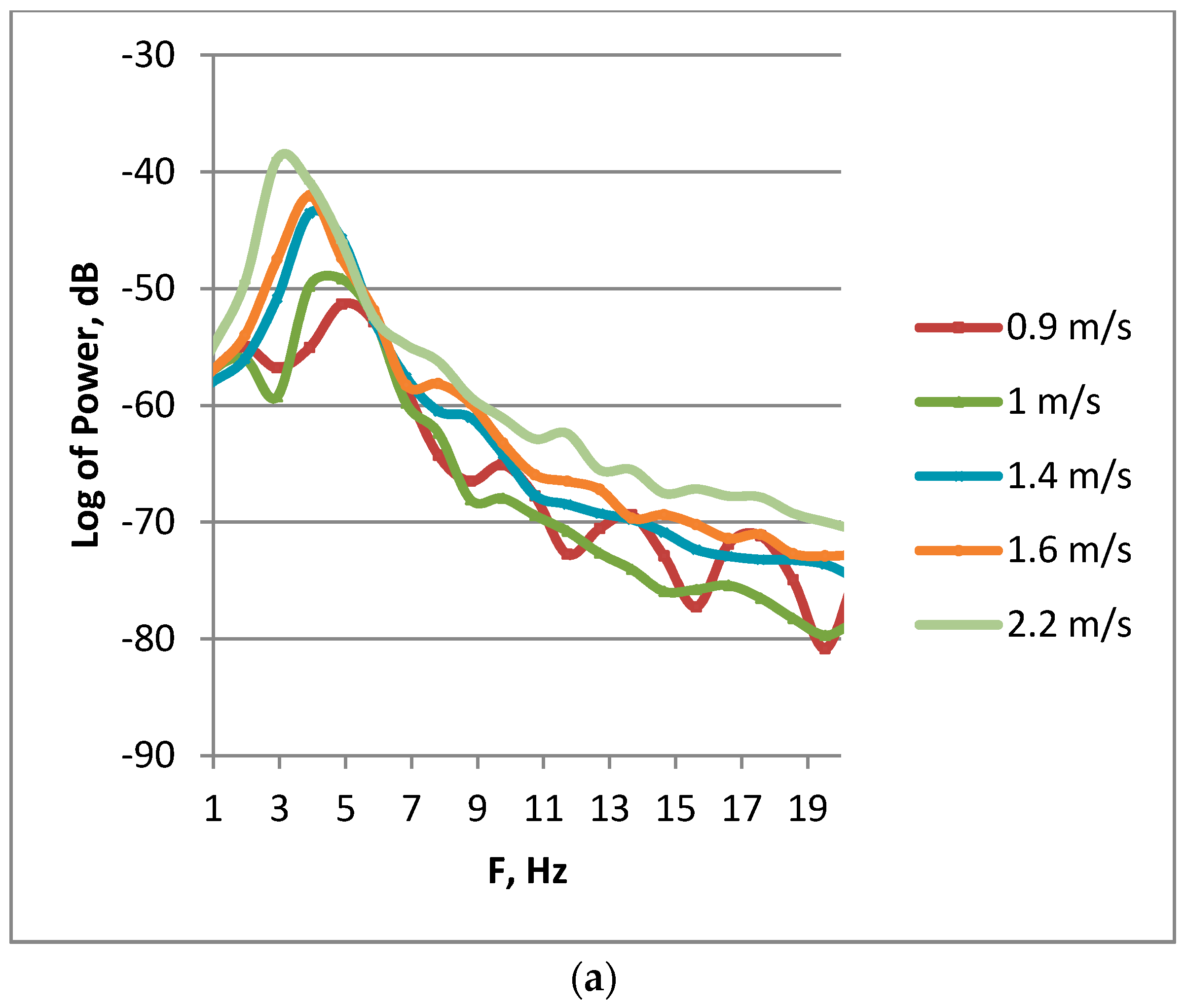
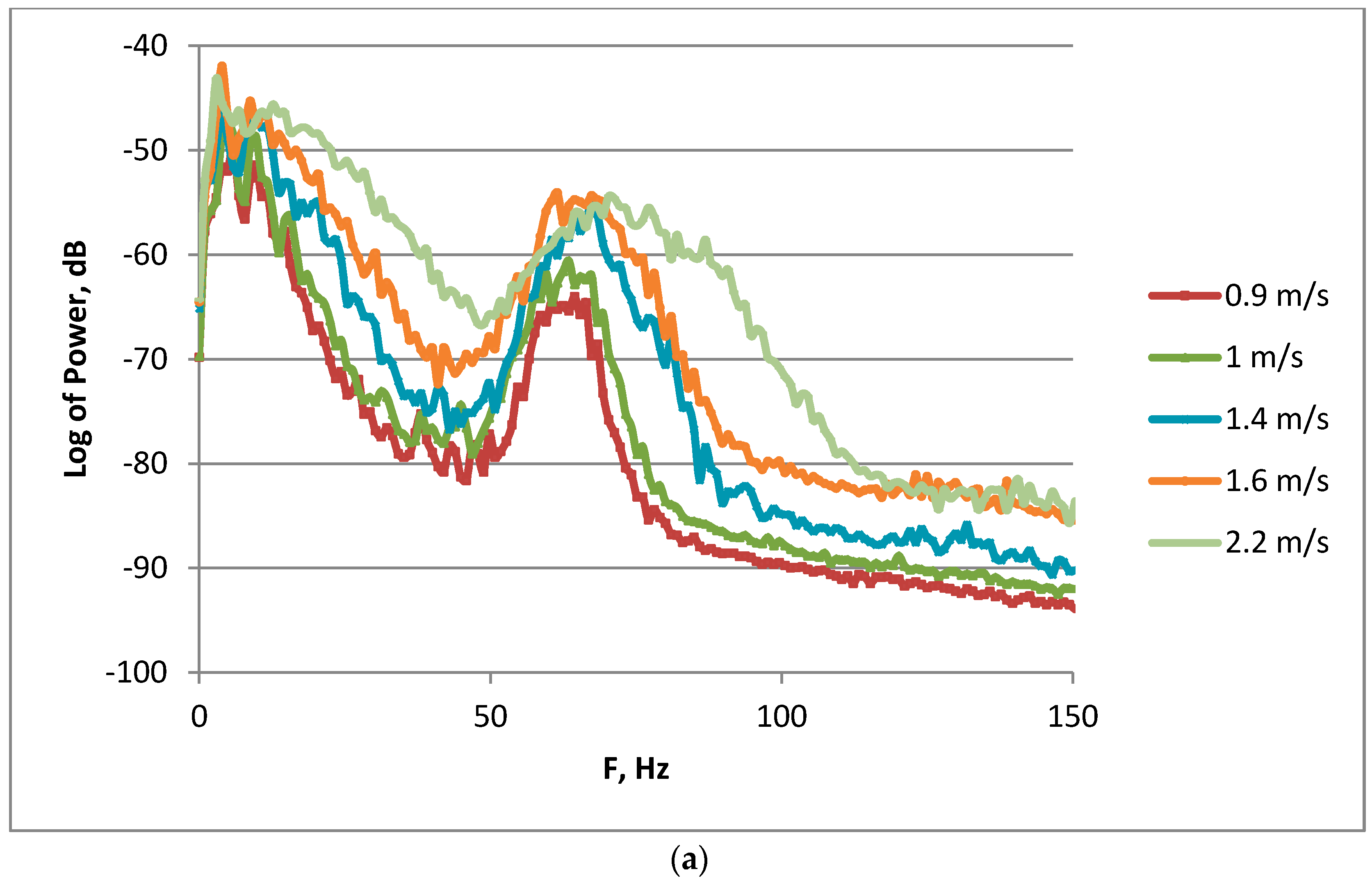
Let us first discuss particularities of wind ripples and of microwave backscattering revealed for the case of purely wind waves in the absence of LF breaking waves. It has been reported before (see, e.g., [6,15,21]) that the spectrum of small-scale wind waves in a cm-mm-wavelength range is determined by free wind ripples directly generated by wind and by bound waves generated on the profile of longer cm-dm-scale waves. The latter can be characterized by an essentially non sinusoidal profile with specific structures, which are toe/bulges and parasitic capillary ripples [9,10]. The toe/bulge structures are located near the crests of basic cm-dm-scale waves, the parasitic ripples are attached to the bulge/toe structures and located on the forward slopes of the basic waves. The nonlinear structures are quasi stationary and move with the phase velocities of the basic waves. The wavelengths of the parasitic capillary ripples are about 6–7 mm near the wave crests [10] and then decrease along the forward slope of the basic waves [9]. The radar Bragg wavelength for the conditions of our experiments is within the spectrum of the parasitic ripples, so the latter can contribute to Ka-band Bragg backscattering at the Doppler frequencies corresponding to the velocities of basic cm-dm-scale waves. The bulge/toe structures have large slopes and can provide backscattering due to quasi specular reflection [12], thus resulting in the decrease of PR-values. The phase velocities of free Bragg waves differ from the velocities of bound waves, and these two types of microwave scatterrers correspond to different Doppler frequencies [6,15,21].
One can retrieve the velocities of microwave scatterers V S C from the measured Doppler shifts using the following relationship:
f D = 1 π k e sin θ V S C
where k e denotes the wavenumber of incident microwave radiation, θ is the incidence angle.
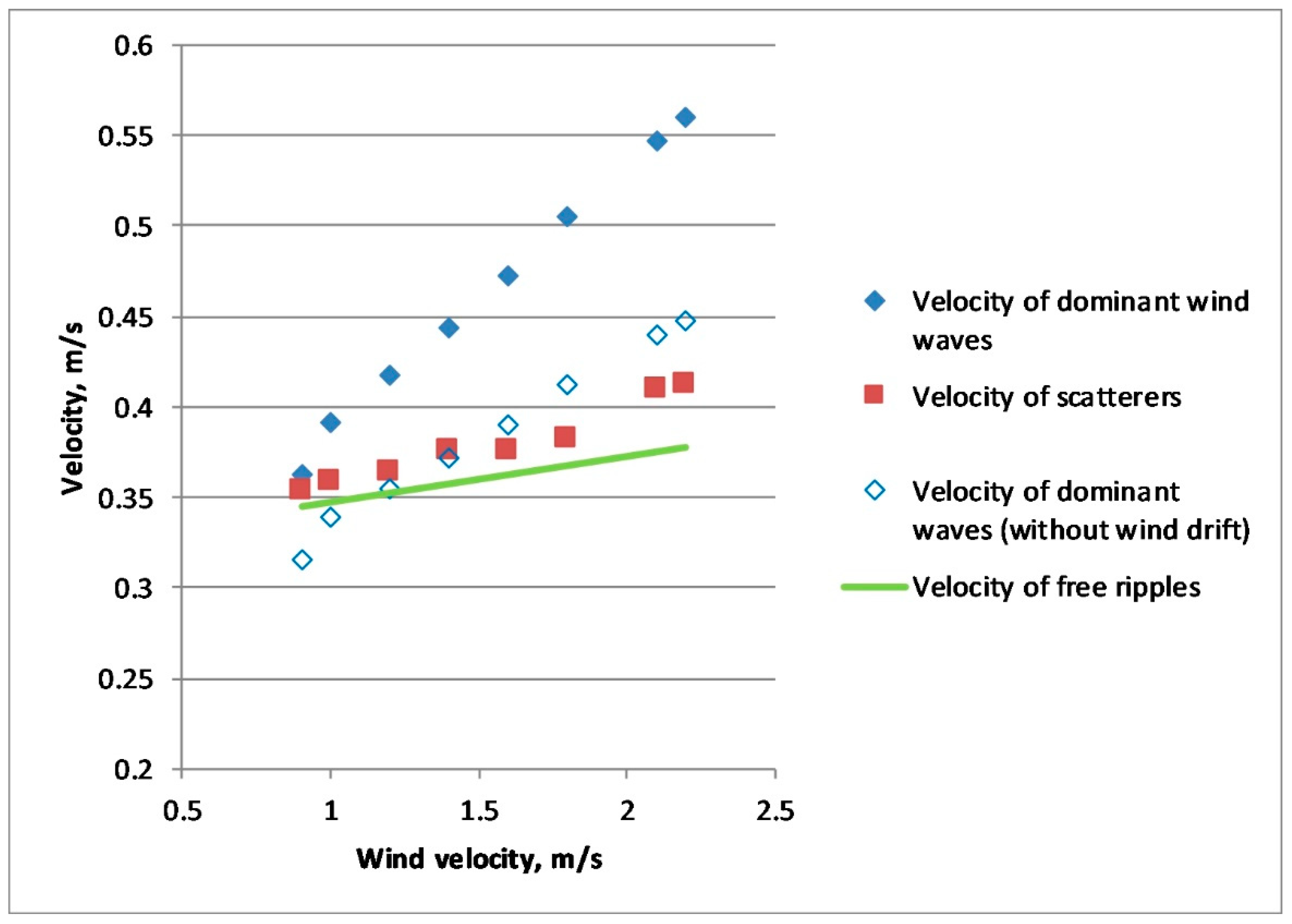
The obtained velocities of scatterers V S C plotted in Figure 13 appeared to be larger than the phase velocities C p ( 2 k e sin θ ) of free GCW at a Bragg wavenumber 2 k e sin θ being summed with wind drift V d r = 0.03 V W 
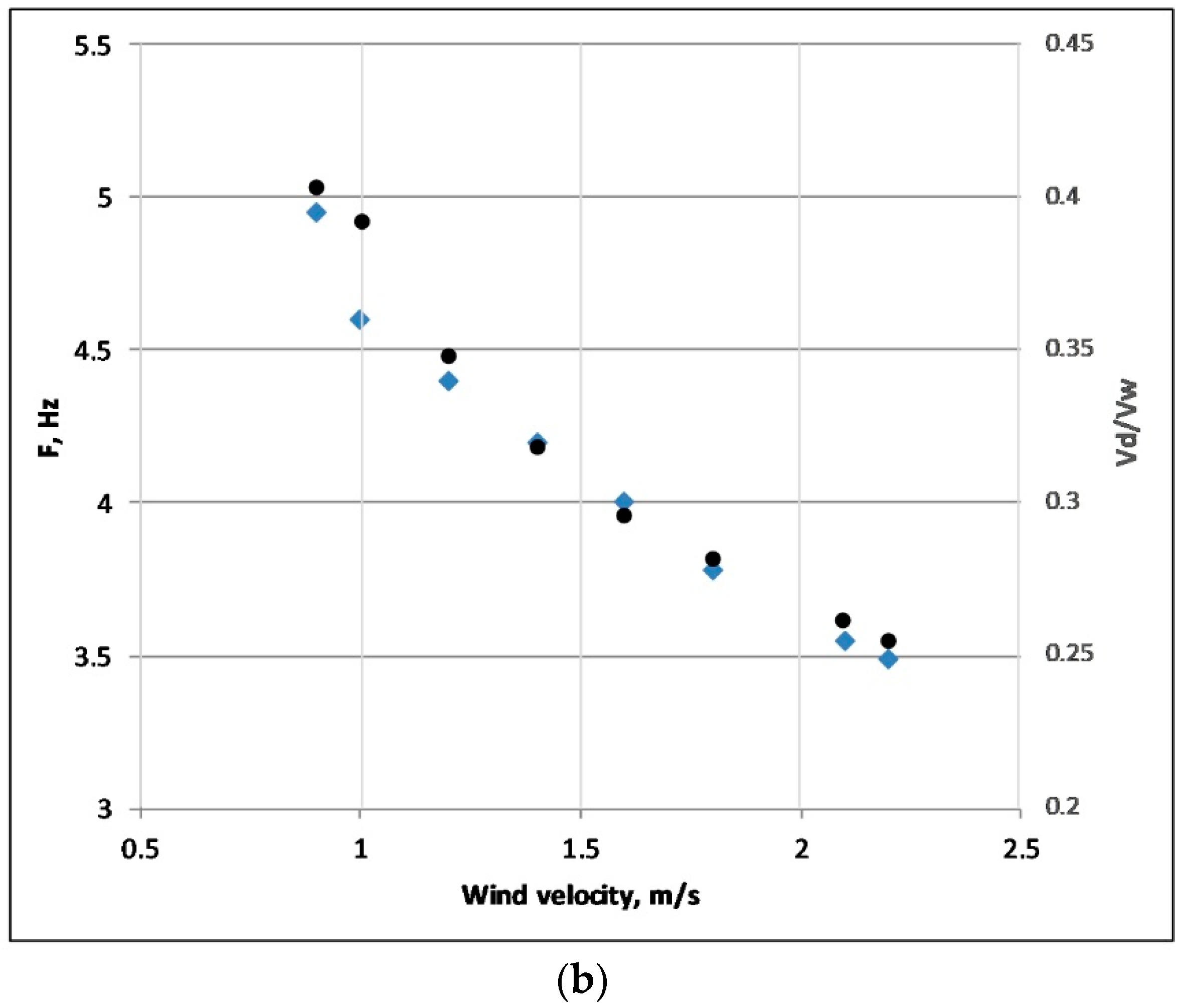
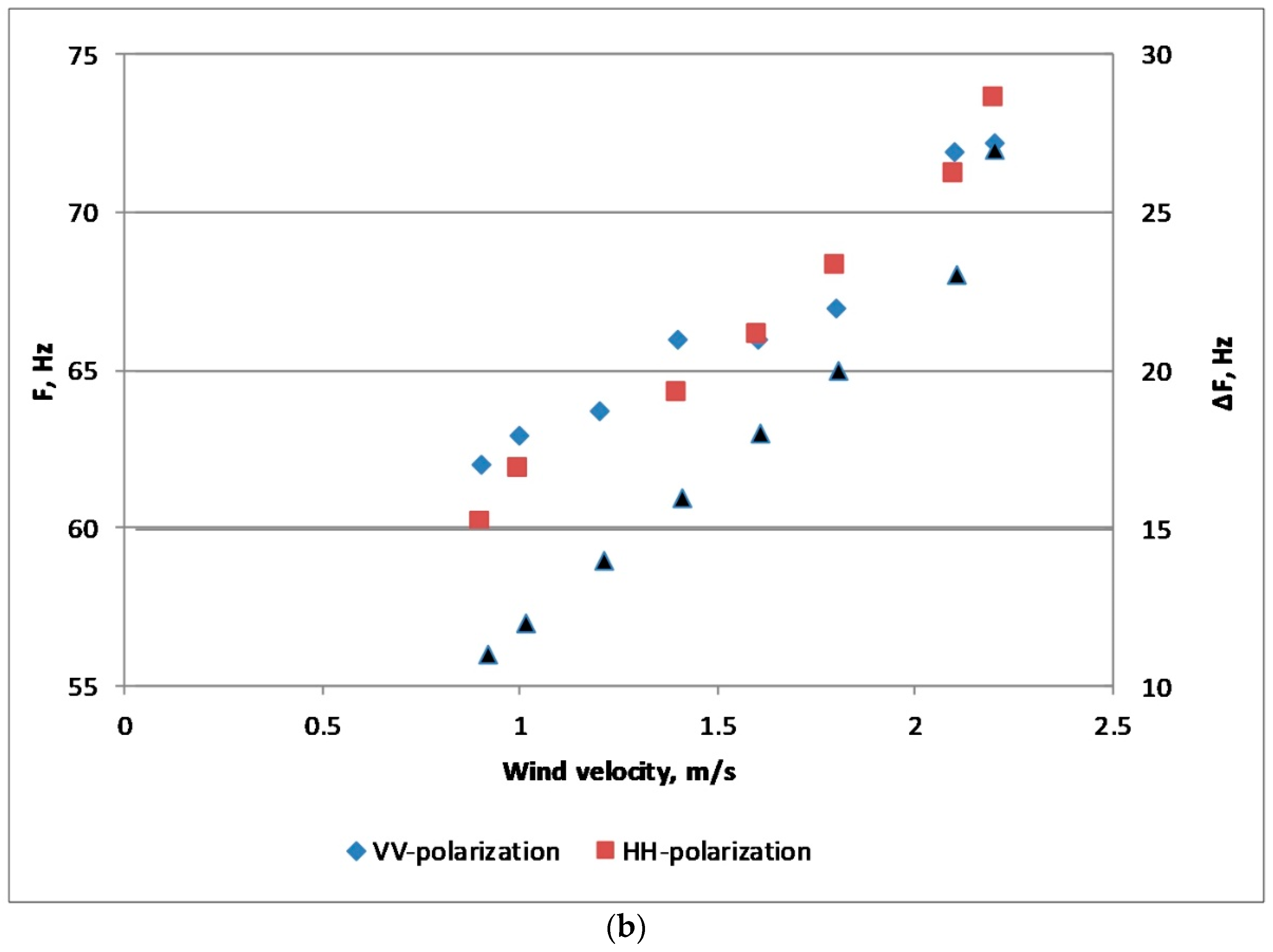
. It is interesting to compare the velocities of scatterers with the velocities of dominant, cm-dm-scale wind waves studied in our experiment. Velocities of the dominant wind waves were retrieved (see Figure 13) using experimentally measured dominant wave frequencies in Figure 6b and the dispersion relation of GCW for two limiting cases: when neglecting the wind drift velocity for the dominant waves and when the drift was considered as 0.03 V W . The two cases were considered because the structure of the wind drift is not well known for the conditions of the tank experiment. The drift may be effective for mm-scale, but less effective for cm-dm-scale waves, since at short fetches and low winds the drift motion may not penetrate deeply in water. Therefore, the resulting wind drift averaged over a vertical layer with a thickness of about the wavelength of cm-dm-scale waves may be smaller than the conventional estimate of 3% of the mean wind speed.
Remarkably, that for all considered cases the velocities of microwave scatterers in Figure 13 are between the velocities of,
  • free linear mm-scale Bragg waves propagating with their intrinsic phase velocity plus wind drift and
  • nonlinear structures (parasitic capillary ripples and bulge/toes) on the profile of cm-dm-scale waves propagating with velocities either modified, or not, by wind drift.
From Figure 13 one therefore can conclude that both types of microwave scatterers contribute to Ka-band radar return.
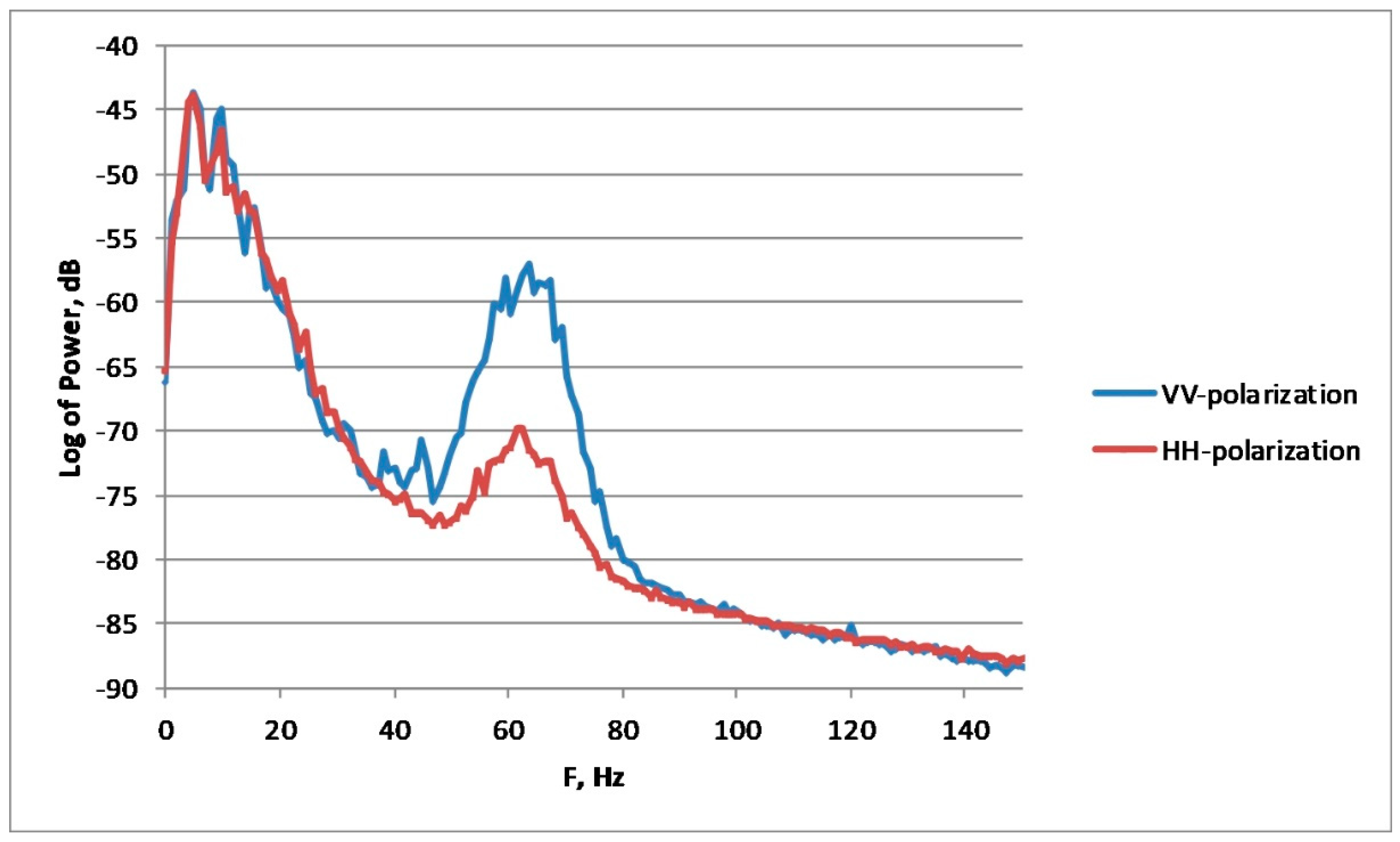
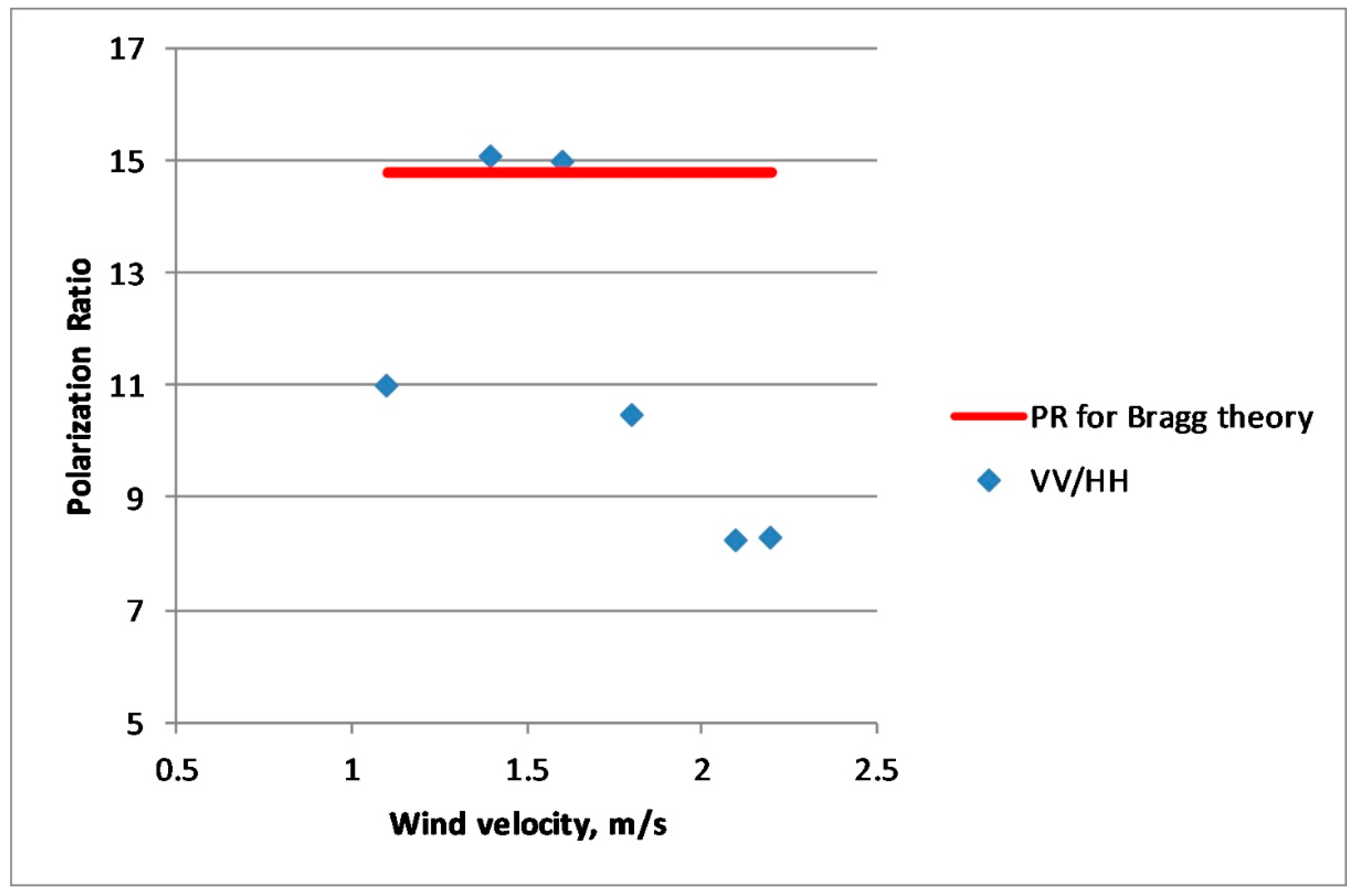
One could expect to get similar conclusions regarding the nature of microwave scattering when analyzing PR-values. The VV/HH polarization ratio for purely Bragg waves under the conditions of our experiment would be about 15, while for non-polarized scattering due to the nonlinear structures it should be close to 1. The PR-values determined in our experiments are located between these two limits as seen in Figure 8, so both Bragg and non-polarized scatterers are contained in wind waves. At the moment it is difficult to estimate accurately the relative contributions of the scatterers in radar return in order to describe the effects of breaking waves on free waves and on the nonlinear structures. So below mostly qualitative characterization of the effect is given.
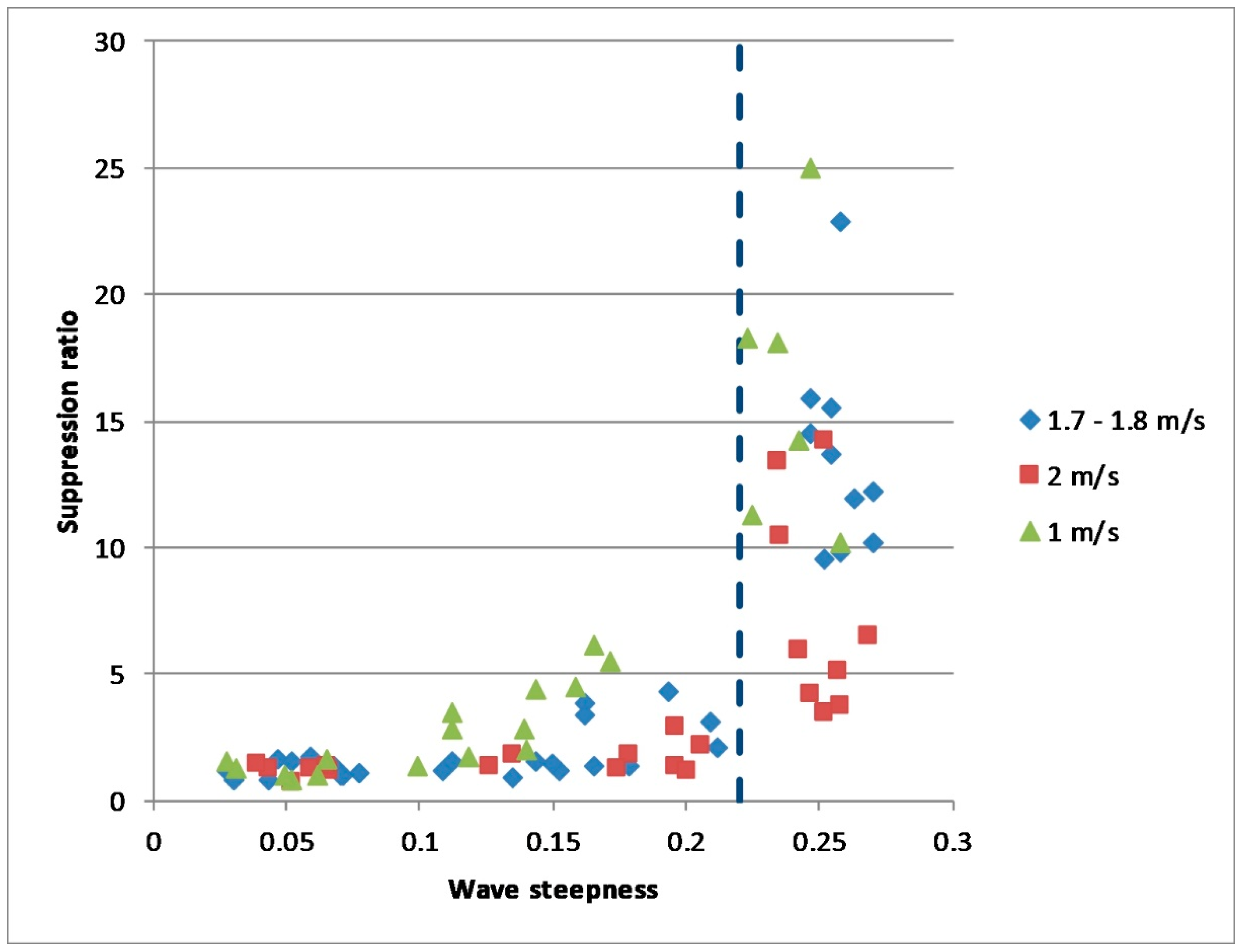
Let us characterize the effect of radar backscatter suppression due to turbulence generated by breaking waves by a suppression ratio (SR) that is a ratio of intensities of radar return before and after the LF wave packet passage. The SR as a function of the wave steepness κ A of intense LF waves ( κ is the wavenumber and A the LF wave amplitude) is shown in Figure 14. The wave steepness values larger than 0.22 correspond to wave breaking while the smaller values are for non-breaking waves. The experiments with non-breaking waves were carried out additionally to the case of breaking waves in order to investigate whether SR depends monotonically on wave steepness. One should emphasize that according to Figure 14 the SR-values for non-breaking waves are not equal to 1 and, consequently, some suppression of radar backscatter occurs, too. The effect of radar backscatter suppression by non-breaking LF waves is not analyzed in this paper and is to be considered elsewhere.
For the steepness larger than 0.22–0.23 the SR rises abruptly to the values of about 15–25. It is natural to assume that the effect of suppression of radar backscatter after the passage of breaking surface waves is due to the attenuation of small-scale wind waves by hydrodynamic turbulence (see [
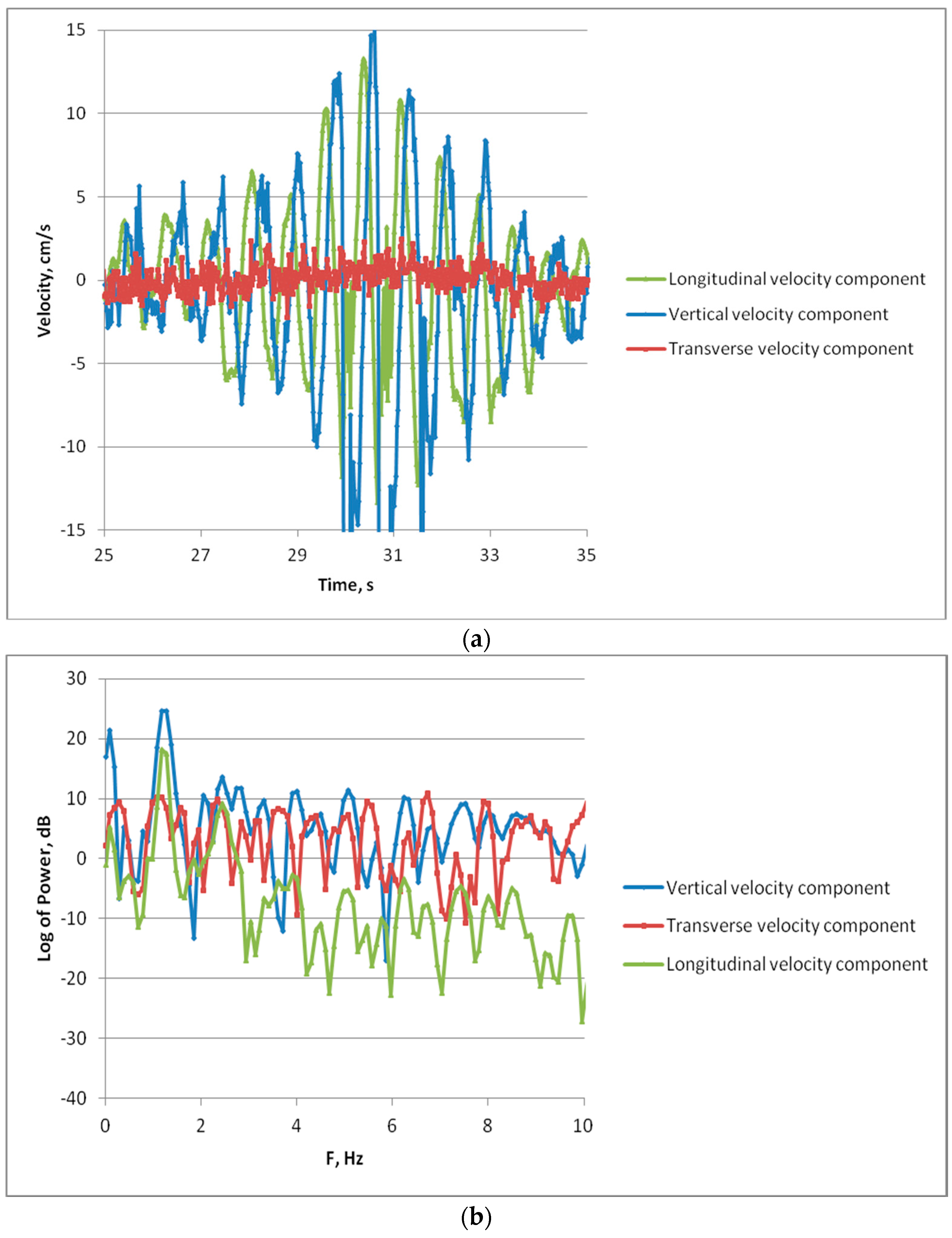
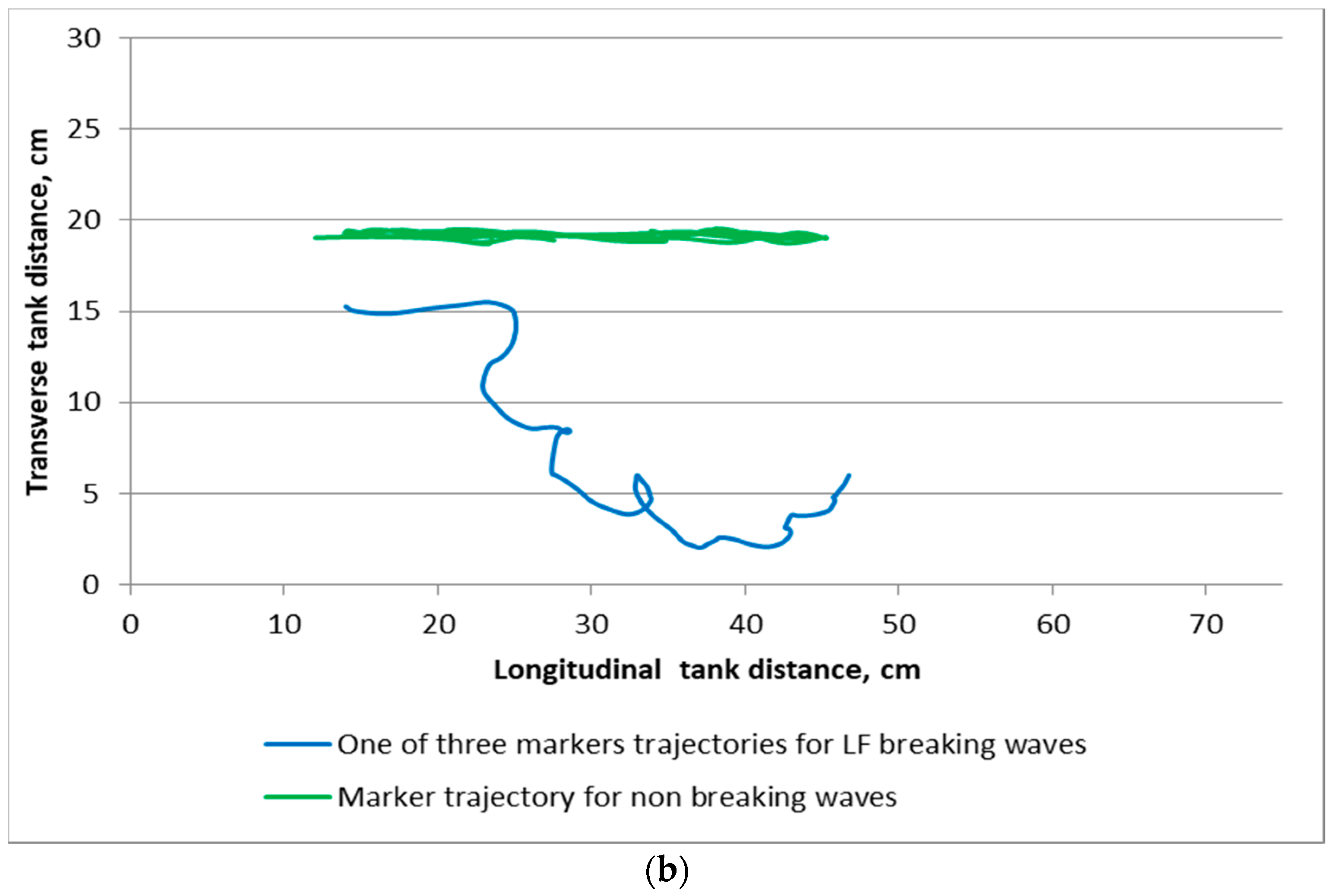
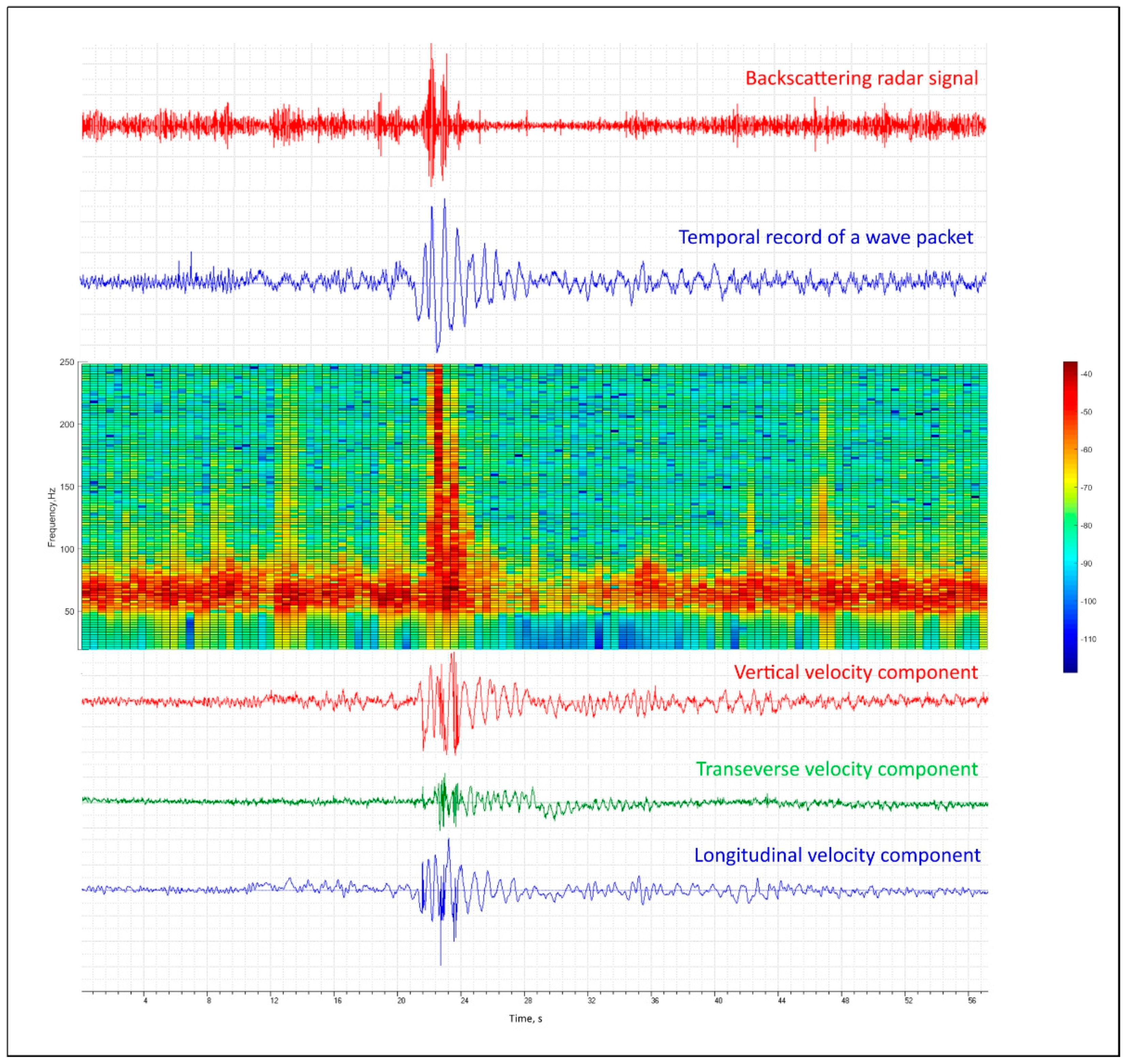
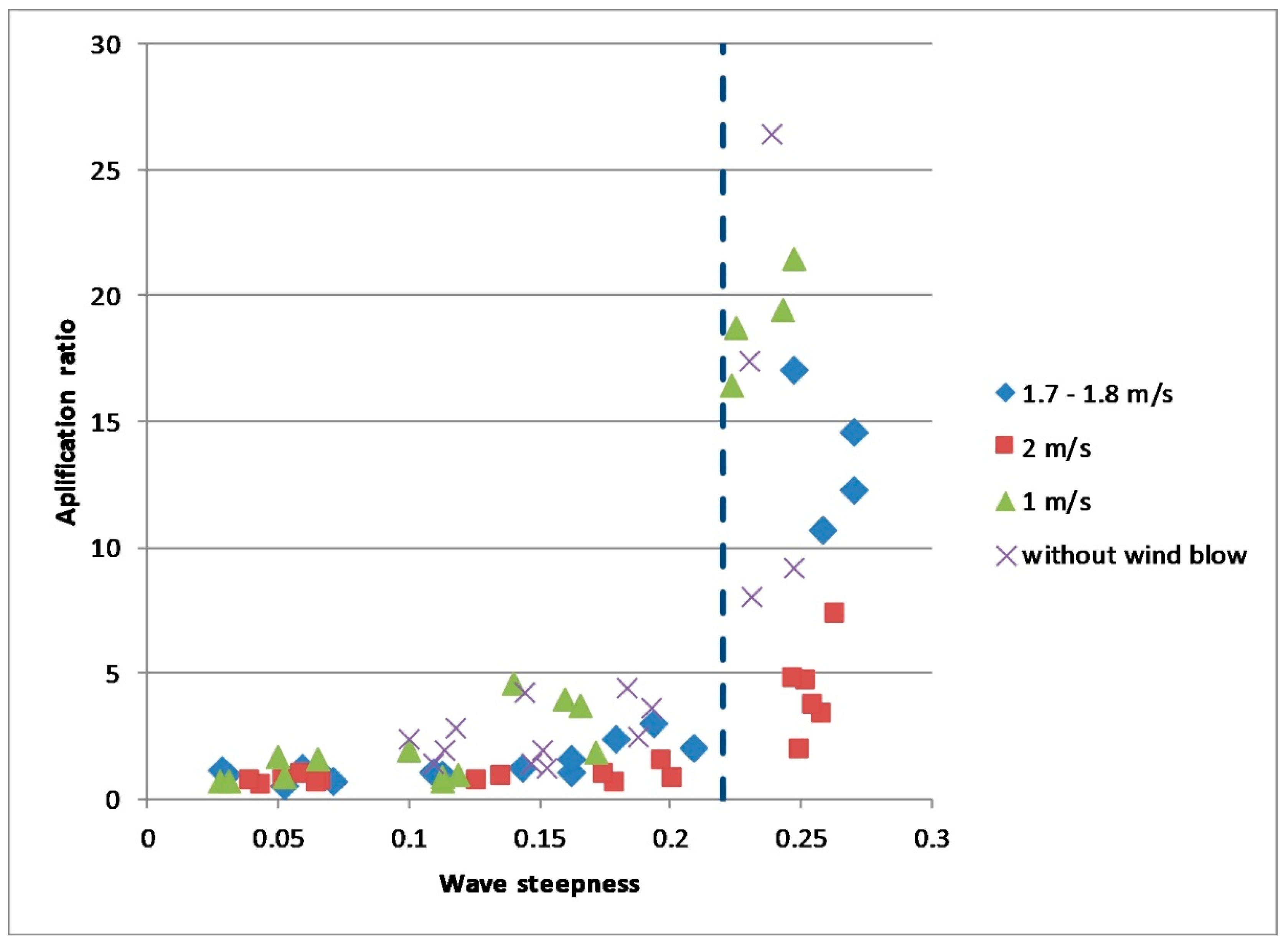
33]) excited as a result of wave crest overturning. The validity of this assumption is confirmed by the appearance of the transverse velocity component which can be associated with turbulence (see Section 3). An amplification ratio (AF) for turbulence that is a ratio of the turbulent kinetic energy after and before the passage of intense wave trains (the latter is practically equal to the noise level) as a function of LF wave steepness is shown in Figure 15.
The energy of turbulence (the intensity of turbulent velocities) was obtained when integrating ADV velocity spectra over a frequency range from 0.5 Hz to 4 Hz and filtering out the long wave frequency peak in the spectrum. Figure 14 and Figure 15 look surprisingly similar, since the general behavior and even the values of the SR are nearly the same as AR, and this similarity is a reliable proof that the radar backscatter suppression is due to turbulence generated by breaking waves and resulting in the enhanced damping of small-scale wind wave and thus suppression of microwave scatterers.
Let us now discuss the effect of radar return suppression. The SR for a Bragg component under an assumption that the Bragg scattering coefficient is not changed after the passage of breaking waves can be estimated as a ratio of wind wave spectrum before and after the LF intense wave train. Similar to how it was done when analyzing the damping of wind waves due to surfactant films (see [35,36]) we can write
S R B r a g g ( γ t e f γ 0 e f ) n
where γ t e f = β 2 γ t , γ 0 e f = β 2 γ 0 , β = β ( k , V W ) denotes the growth rate in the of wind waves with wavenumber k , γ t and γ 0 = 2 ν k 2 the wave amplitude damping coefficients in the presence of turbulence and on calm clean water, respectively, ν is the kinematic water viscosity. In (2) n = 1 when β < γ t , γ 0 and wind waves are generated due to Phillips’ mechanism, and n = 1 when β > γ t , γ 0 and Miles’ mechanism of wave excitation dominates [37].
The damping coefficient due to turbulence γ t can be expressed similarly to γ 0 , but substituting ν by the eddy viscosity ν t C t u t 2 ¯ l t . Here u t 2 ¯ is r.m.s. turbulent velocity, l t is an integral scale of turbulence, C t is some empirical coefficient. In our recent paper [33] the damping due to turbulence was studied in laboratory experiment for surface waves in a frequency range from about 3 to 13 Hz and ν t was found to have a maximum for wavelengths comparable to the turbulent scale and decreased to the values of order 0.05 cm2/s at frequencies about 13 Hz. The turbulent scale l t for breaking waves can be estimated as about 0.1 of the breaking wavelength (see [26]), so that for the case of our experiments l t 7 cm. Extrapolating the values of the eddy viscosity obtained in [33] for Ka-band Bragg wavelengths we can set ν t 0.1 cm2/s. Then the SR-values for Bragg scattering at very low winds about 2 m/s and less can be estimated as S R B r a g g 10 . In order to estimate SR, one needs to take into account also non polarized scattering.
Typically, PR values are larger than 1 and smaller than those predicted by Bragg theory thus indicating that Bragg and NP component contributions can be comparable to each other. This was confirmed in a number of previous laboratory experiments (see Section 1) and in our study, as well as in field observations, too (see, e.g., [38]).
NP scattering has been assumed in [4] as quasi-specular reflection from small-scale facets. At moderate radar incidence angles the NP component depends exponentially on the slope variance of wind waves which are longer than (3–5) the lengths of microwaves, i.e., by cm-dm-scale wind waves. NP backscattering decreases dramatically when the slope variance even weakly decreases. According to our experimental data the cm-dm-wave slope variance after the passage of breaking waves is at least 0.5–0.7 of the background wind wave variance, so that NP radar return after wave breaking becomes exponentially small and can be neglected compared with the background NP component. Assuming that Bragg and NP scattering components are comparable to each other for the background wind waves one can write the total SR as
S R = σ 0 σ t = σ B r a g g 0 + σ N P 0 σ B r a g g t + σ N P t S R B r a g g ( 1 + σ N P 0 σ B r a g g 0 ) = S R B r a g g A
where σ 0 and σ t are NRCS for background wind waves and for turbulent area, respectively, the coefficient A is about 2 for typical wind wave conditions, when σ B r a g g 0 σ N P 0 . Based on the above estimates of PR and S R B r a g g one can conclude that SR-values determined by (3) are consistent with experiment.
Let us further speculate to extend the results of our laboratory experiments to real sea conditions. Strong wave breaking occurs at moderate wind velocities of 6–7 m/s and higher. The eddy viscosity in the breaking zones according to the results of laboratory studies [33] can be in the range of about (0.1–1) cm2/s. Corresponding damping coefficient values for Ka-band Bragg waves exceed the wind wave growth rates even for wind velocities of about 8–10 m/s, and the model [35,36] is not applicable for correct estimates of wind wave damping. However, at similar conditions in field experiments with film slicks when the model [35,36] could not be applied the damping ratio in slicks exceeded 10, and we can assume that the SR-values due to turbulence can be of the same order. For X-band Bragg waves and v t ~ 0.1 cm2/s one can obtain S R B r a g g to be about 3, and based on (3) one can estimate SR-values of about 6. For the high value of eddy viscosity, the model [35,36] fails again, but we can expect again that the SR-values are to be larger than 10. Therefore, we believe that the effect of backscatter suppression after wave breaking can be reliably recorded in real sea conditions when using radar with very high spatial resolution. To analyze the effect of radar backscatter suppression in more detail one needs to develop semi empirical models of wave damping due to turbulence as well as to use improved models of wind wave suppression due to turbulence. This can be a subject of future studies
An alternative explanation of the effect of wind wave suppression due to breaking waves can be given following [28]. As it was mentioned above a coherent vortex is formed in water as a result of wave breaking. It was argued in [28] that short surface waves propagating on the nonuniform surface current associated with the vortex are weakened on an accelerating upstream current and are enhanced or even blocked on a decelerating current at the downstream part of the vortex. Let us consider this mechanism for the conditions of our experiments. According to [28] typical current velocities in the vortex are about 0.04 C , where C is the phase velocity of breaking waves. Therefore, the current velocity in the vortex in our experiments should be about 5 cm/s. The amplitude a of a short gravity wave co-directional with a non-uniform current which velocity is growing from zero to U can be described by the following formula (see [37])
a / a 0 = 2 ( 1 + 1 + 4 U c 0 ) ( 1 + 4 U c 0 ) 1 / 4
where a 0 is the wave amplitude at the point where U = 0 .
For quasi monochromatic surface waves propagating in the current direction one has to set U > 0 in (4) and for short cm-scale surface waves the amplitude decreases by two to three times compared to a 0 . The effect is to be even smaller for cm-mm-scale waves due to viscous dissipation of these waves. We thus can conclude that the effect of attenuation of wind waves when propagating on non-uniform mean currents generated by the vortex is somewhat less than the suppression due to turbulence. As for the effect of blocking of wind waves at the downstream part of the vortex, it was not observed in the radar signal. One of the reasons is that the effect could be masked by subsequent waves in the LF breaking packet.
Finally, it should be also noted that the obtained SR-values are consistent with the Damping Ratio values (Contrasts) in experiments on microwave radar probing of surface films. Radar contrasts of oil slicks can vary in a wide range depending on wind speed and physical characteristics of surfactant films. However, typical Ka-band contrast values at low-to moderate winds of 4–6 m/s either for typical monomolecular films or oil spills (see [35,36,39]) are comparable with the SR-values shown in Figure 14.

5. Conclusions

Wave tank studies of the action of wave breaking on microwave scattering from the water surface have been carried out. The methodology of the experiments included simultaneous measurements of microwave backscattering with a Ka-band scatterometer, surface waves with wire gauges, velocities in the upper water layer and on the water surface with an acoustic Doppler velocimeter (ADV) and video recording of surface float trajectories.
Wind waves were generated at low wind velocities and short fetches and their wavelengths were typically smaller than 15–20 cm. Wave trains of longer waves of decimeter-to-meter wavelengths were generated using a mechanical wave maker with linearly varying frequency, so the wave trains were compressed at a given distances due to dispersive focusing and short wave packets were formed with 1 or 2 most intense individual waves with breaking crests.
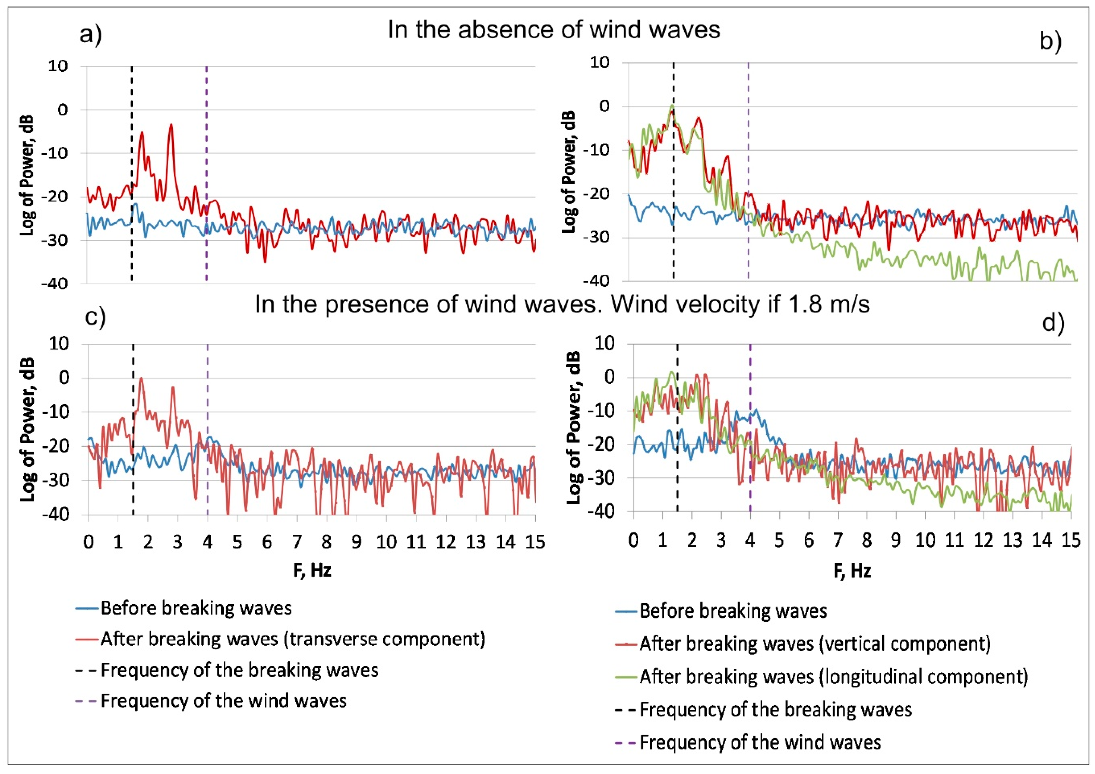
The Doppler spectrum of wind waves in the absence of breaking waves was centered between the frequencies of Bragg waves moving with their intrinsic phase velocities plus wind drift velocity and the frequencies corresponding to the phase velocities of dominant wind waves. This demonstrated that wind ripples can be considered as a mixture of free mm-scale Bragg waves and of bound waves appeared due to nonlinearity on the profile of cm-dm-scale wind waves. The conclusion was supported by the measurements of co-polarized backscatter at vertical (VV) and horizontal (HH) polarization, which demonstrated that the polarization VV/HH-ratio was in between the values for purely Bragg scattering and for non-polarized scattering, the latter can be associated with the nonlinear bulge/toe-structures on the cm-dm-scale wind waves.
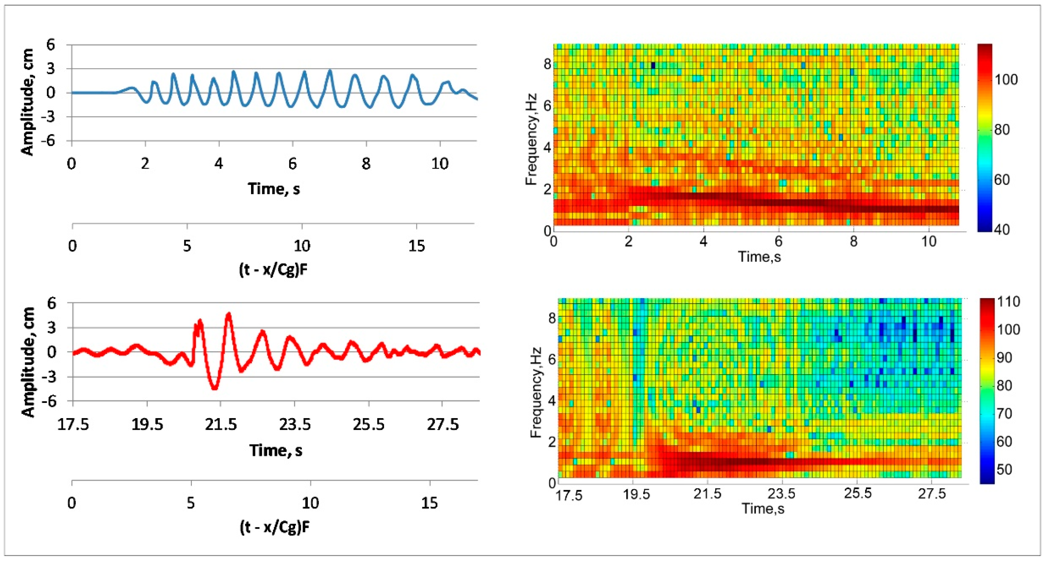
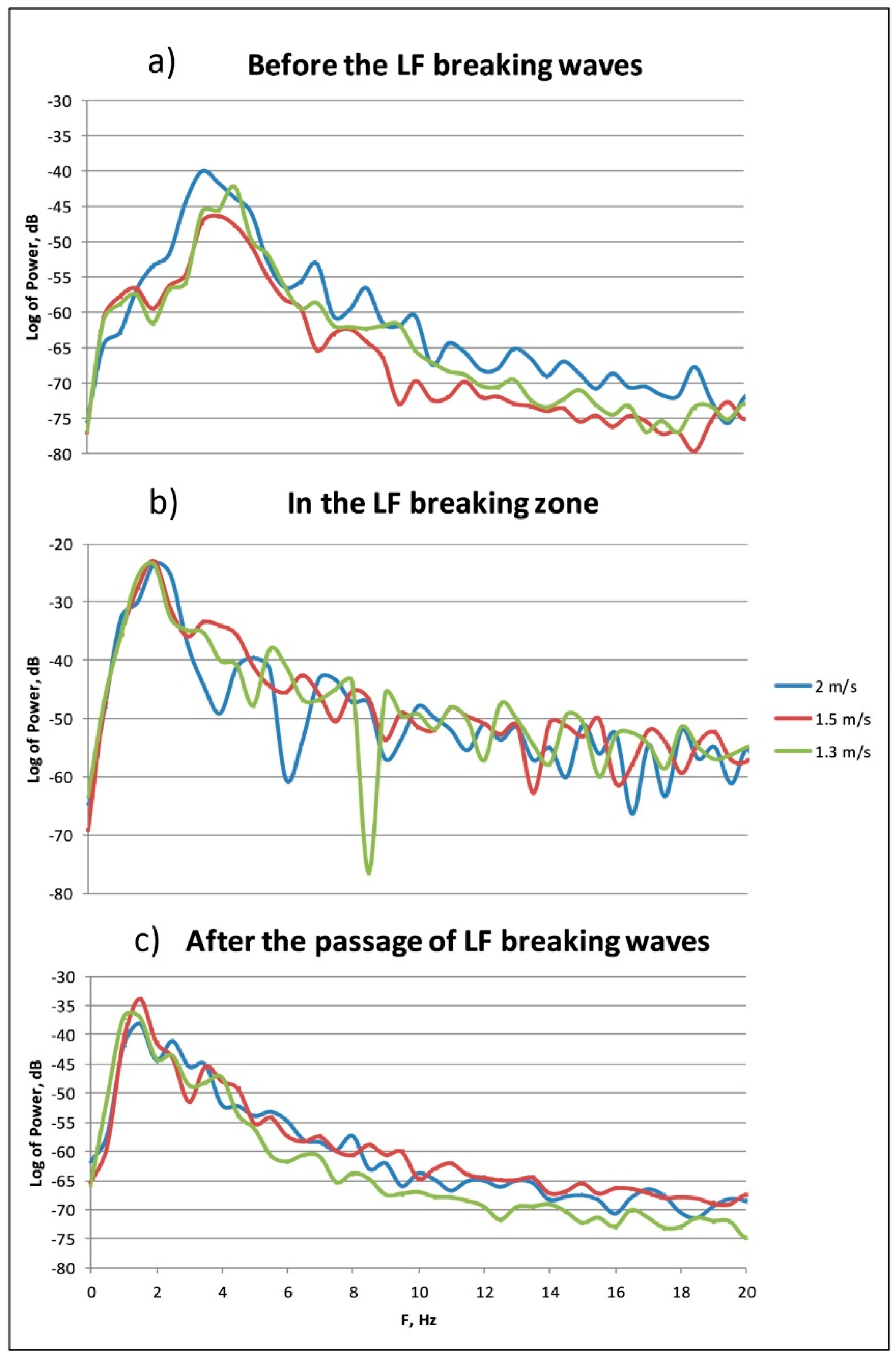
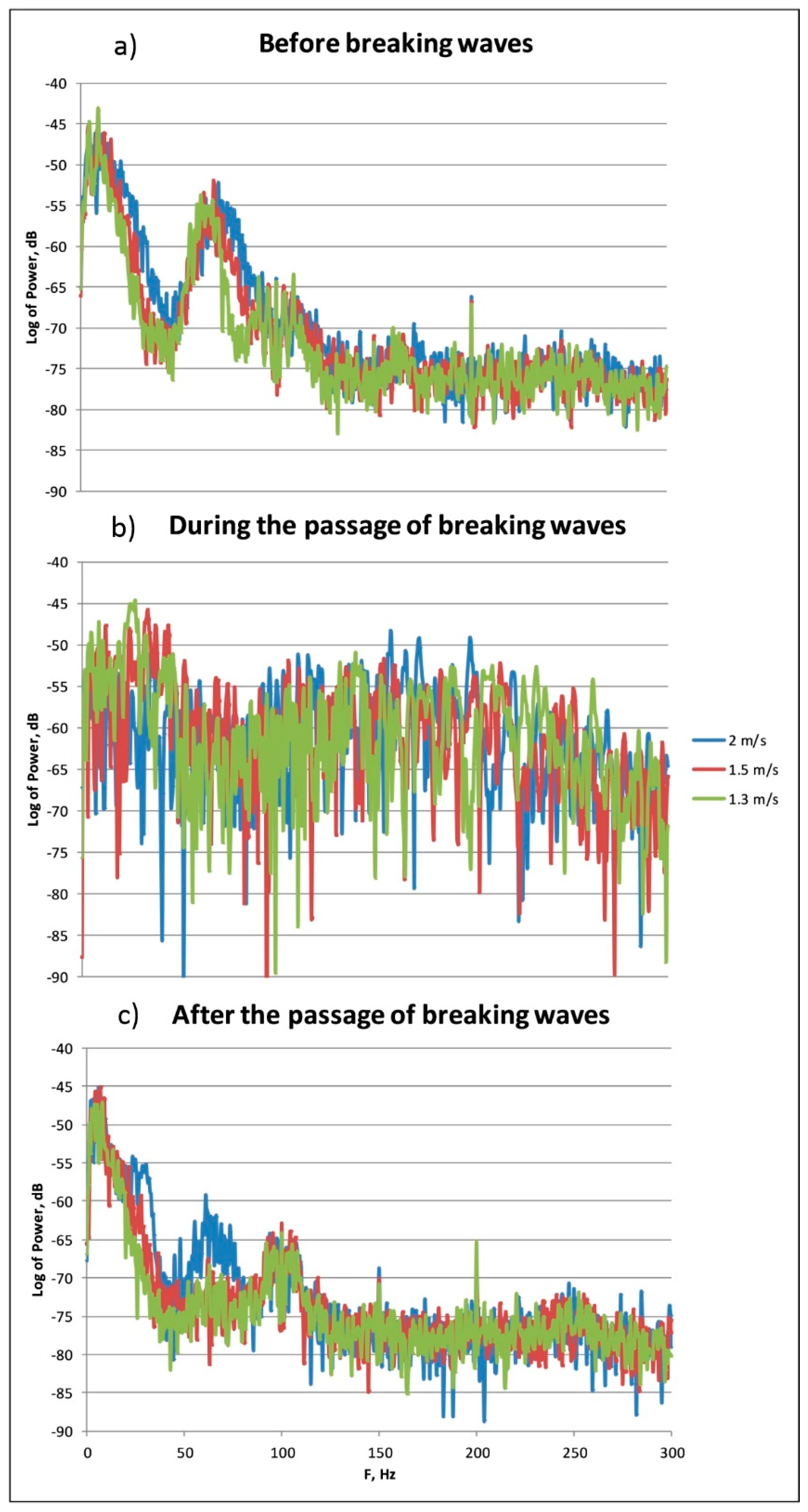
Radar backscatter during the passage of breaking waves was strongly intensified and the radar Doppler spectrum became very wide. After the passage of a packet of breaking waves the radar Doppler spectrum was located in the same frequency range as for the background wind waves, but the intensity of radar backscattering was reduced substantially by about an order of magnitude. After some time, the radar backscatter tended to be at the background level.
Wire gauge measurements demonstrated that the wind wave height variance dropped after the passage of breaking waves and then it was restored to the background values in consistency with the radar data.
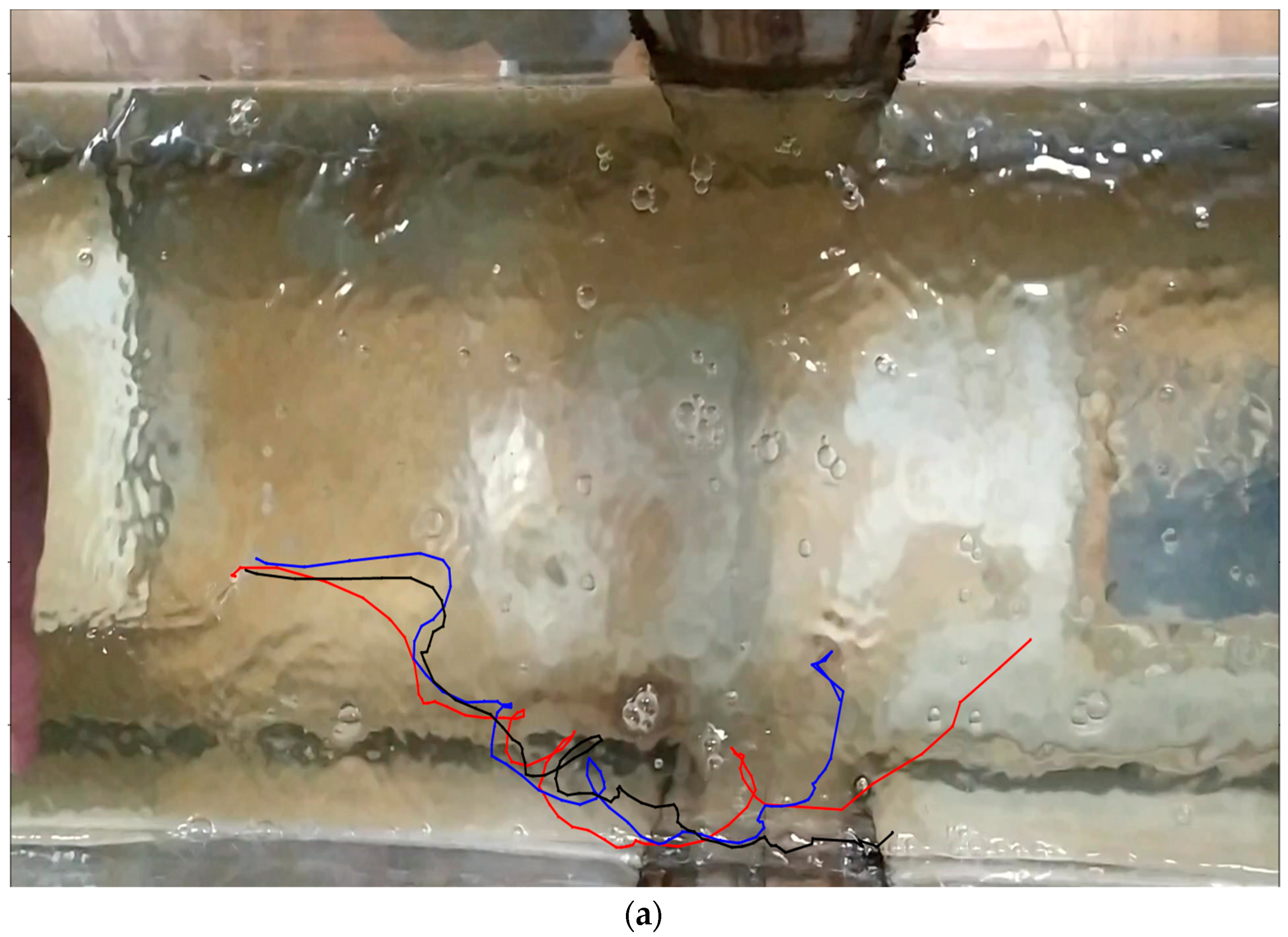
Finally, ADV measurements, as well as analysis of trajectories of surface floats, demonstrated that turbulence was generated during wave breaking and remained in the breaking area for some time, resulting in the enhanced damping of wind waves and thus in the suppression of radar backscatter after the passage of breaking waves.
One thus can conclude that the effect of Ka-band radar backscatter reduction after the passage of breaking waves can be explained as a result of suppression of small-scale wind waves by hydrodynamic turbulence generated due to wave breaking.
Theoretical estimates of the radar backscatter suppression ratio were shown to be consistent with the experiment.
The revealed effect of suppression of radar backscatter after strong wave breaking can be erroneously regarded as radar return suppression due to surface films, wind shadowing and others processes, and should be taken into account when interpreting signatures in radar imagery of the sea surface.

Author Contributions

S.A.E. conceived experiments, analyzed the results and wrote the article, V.A.D. and I.A.K. conducted experiments, processed the data, I.A.S. analyzed the results. All authors have read and agreed to the published version of the manuscript.

Funding

This research was funded by the Russian Science Foundation (Project RSF 18-17-00224). The methodology of experiments (Section 2.3) was developed in the frame of the Project 0729-2020-0037 “Goszadanije”.

Acknowledgments

We are grateful to A. Kupaev for his help in experiment. We are very thankful to anonymous reviewers for their valuable comments.

Conflicts of Interest

The authors declare no conflict of interest.

References

  1. Valenzuela, G.R. Theories for the interaction of electromagnetic and oceanic waves?—A review. Boundary-Layer Meteorol. 1978, 13, 61–85. [Google Scholar] [CrossRef]
  2. Bass, F.G.; Fuks, M. Wave Scattering from Statistically Rough Surfaces; Pergamon: Oxford, UK, 1979; p. 540. ISBN 9781483187754. [Google Scholar]
  3. Phillips, O.M. Radar Returns from the Sea Surface—Bragg Scattering and Breaking Waves. J. Phys. Oceanogr. 1988, 18, 1065–1074. [Google Scholar] [CrossRef]
  4. Kudryavtsev, V.; Hauser, D.; Caudal, G.; Chapron, B. A semiempirical model of the normalized radar cross-section of the sea surface 1. Background model. J. Geophys. Res. Space Phys. 2003, 108, 8054. [Google Scholar] [CrossRef] [Green Version]
  5. Kudryavtsev, V.N.; Chapron, B.; Myasoedov, A.G.; Collard, F.; Johannessen, J.A.; Myasoedov, A.G.; Johannessen, J.A. On Dual Co-Polarized SAR Measurements of the Ocean Surface. IEEE Geosci. Remote Sens. Lett. 2012, 10, 761–765. [Google Scholar] [CrossRef]
  6. Longuet-Higgins, M.S.; Cleaver, R.P. Crest instabilities of gravity waves. Part 1. The almost-highest wave. J. Fluid Mech. 1994, 258, 115. [Google Scholar] [CrossRef]
  7. Duncan, J.H. Spilling breakers. Annu. Rev. Fluid Mech. 2001, 33, 519–547. [Google Scholar] [CrossRef]
  8. Qiao, H.; Duncan, J.H. Gentle spilling breakers: Crest flow-field evolution. J. Fluid Mech. 2001, 439, 57–85. [Google Scholar] [CrossRef]
  9. Longuet-Higgins, M.S. Parasitic capillary waves: A direct calculation. J. Fluid Mech. 1995, 301, 79. [Google Scholar] [CrossRef]
  10. Yermakov, S.A.; Ruvinsky, K.D.; Salashin, S.G. Local correlation of the characteristics of ripples on the crest of capillary gravity waves with their curvature. Izv. Atmos. Ocean. Phys. 1988, 24, 561–563. [Google Scholar]
  11. Hansen, M.W.; Kudryavtsev, V.; Chapron, B.; Brekke, C.; Johannessen, J.A. Wave Breaking in Slicks: Impacts on C-Band Quad-Polarized SAR Measurements. IEEE J. Sel. Top. Appl. Earth Obs. Remote Sens. 2016, 9, 4929–4940. [Google Scholar] [CrossRef] [Green Version]
  12. Ermakov, S.A.; Sergievskaya, I.A.; da Silva, J.C.; Kapustin, I.A.; Shomina, O.V.; Kupaev, A.V.; Molkov, A.A. Remote Sensing of Organic Films on the Water Surface Using Dual Co-Polarized Ship-Based X-/C-/S-Band Radar and TerraSAR-X. Remote Sens. 2018, 10, 1097. [Google Scholar] [CrossRef] [Green Version]
  13. Sergievskaya, I.A.; Ermakov, S.A.; Ermoshkin, A.V.; Kapustin, I.A.; Molkov, A.A.; Danilicheva, O.A.; Shomina, O.V. Modulation of Dual-Polarized X-Band Radar Backscatter Due to Long Wind Waves. Remote Sens. 2019, 11, 423. [Google Scholar] [CrossRef] [Green Version]
  14. Kwoh, D.; Lake, B. A deterministic, coherent, and dual-polarized laboratory study of microwave backscattering from water waves, Part I: Short gravity waves without wind. IEEE J. Ocean. Eng. 1984, 9, 291–308. [Google Scholar] [CrossRef]
  15. Gade, M.; Alpers, W.; Ermakov, S.A.; Hühnerfuss, H.; Lange, P.A. Wind-wave tank measurements of bound and freely propagating short gravity-capillary waves. J. Geophys. Res. Space Phys. 1998, 103, 21697–21709. [Google Scholar] [CrossRef]
  16. Ebuchi, N.; Kawamura, H.; Toba, Y. Physical processes of microwave backscattering from laboratory wind wave surfaces. J. Geophys. Res. Space Phys. 1993, 98, 14669. [Google Scholar] [CrossRef]
  17. Plant, W.J.; Keller, W.C.; Hesany, V.; Hara, T.; Bock, E.; Donelan, M.A. Bound waves and Bragg scattering in a wind-wave tank. J. Geophys. Res. Space Phys. 1999, 104, 3243–3263. [Google Scholar] [CrossRef]
  18. Rozenberg, A.D.; Quigley, D.C.; Melville, W.K. Laboratory study of polarized microwave scattering by surface waves at grazing incidence: The influence of long waves. IEEE Trans. Geosci. Remote Sens. 1996, 34, 1331–1342. [Google Scholar] [CrossRef] [Green Version]
  19. Walker, D.T.; Lyzenga, D.R.; Ericson, E.A.; Lund, D.E. Radar backscatter and surface roughness measurements for stationary breaking waves. In Proceedings of the Royal Society A: Mathematical, Physical and Engineering Sciences; The Royal Society: London, UK, 1996; Volume 452, pp. 1953–1984. [Google Scholar]
  20. Rozenberg, A.D. Laboratory study of the fine structure of short surface waves due to breaking: Two-directional wave propagation. J. Geophys. Res. Space Phys. 2005, 110. [Google Scholar] [CrossRef]
  21. Ermakov, S.A.; Kapustin, I.A.; Sergievskaya, I.A. On peculiarities of scattering of microwave radar signals by breaking gravity-capillary waves. Radiophys. Quantum Electron. 2012, 55, 453–461. [Google Scholar] [CrossRef]
  22. Zuo, L.; Li, M.; Zhang, X.; Wang, Y.; Wu, Y. An Efficient Method for Detecting Slow-Moving Weak Targets in Sea Clutter Based on Time–Frequency Iteration Decomposition. IEEE Trans. Geosci. Remote Sens. 2012, 51, 3659–3672. [Google Scholar] [CrossRef]
  23. Donelan, M.A.; Haus, B.K.; Reul, N.; Plant, W.J.; Stiassnie, M.; Graber, H.C.; Brown, O.B.; Saltzman, E.S. On the limiting aerodynamic roughness of the ocean in very strong winds. Geophys. Res. Lett. 2004, 31. [Google Scholar] [CrossRef] [Green Version]
  24. Bye, J.A.T.; Jenkins, A.D. Drag coefficient reduction at very high wind speeds. J. Geophys. Res. Space Phys. 2006, 111, 3. [Google Scholar] [CrossRef]
  25. Donnelly, W.J.; Carswell, J.R.; McIntosh, R.E.; Chang, P.S.; Wilkerson, J.; Marks, F.D.; Black, P.G. Revised ocean backscatter models at C and Ku band under high-wind conditions. J. Geophys. Res. Space Phys. 1999, 104, 11485–11497. [Google Scholar] [CrossRef]
  26. Rapp, R.J.; Melville, W.K. Laboratory measurements of deep-water breaking waves. Philos. Trans. R. Soc. London. Ser. A Math. Phys. Sci. 1990, 331, 735–800. [Google Scholar] [CrossRef] [Green Version]
  27. Ölmez, H.S.; Milgram, J.H. An experimental study of attenuation of short water waves by turbulence. J. Fluid Mech. 1992, 239, 133–156. [Google Scholar] [CrossRef]
  28. Melville, W.K.; Veron, F.; White, C.J. The velocity field under breaking waves: Coherent structures and turbulence. J. Fluid Mech. 2002, 454, 203–233. [Google Scholar] [CrossRef] [Green Version]
  29. Milgram, J.H. Short wave damping in the simultaneous presence of a surface film and turbulence. J. Geophys. Res. Space Phys. 1998, 103, 15717–15727. [Google Scholar] [CrossRef]
  30. Teixeira, M.A.C.; Belcher, S.E. On the distortion of turbulence by a progressive surface wave. J. Fluid Mech. 2002, 458, 229–267. [Google Scholar] [CrossRef]
  31. Beya, J.; Peirson, W.; Banner, M. Attenuation of gravity waves by turbulence. Coast. Eng. Proc. 2011, 1, 1–10. [Google Scholar] [CrossRef]
  32. Gutiérrez, P.; Aumaître, S. Surface waves propagating on a turbulent flow. Phys. Fluids 2016, 28, 025107. [Google Scholar] [CrossRef]
  33. Shomina, O.; Kapustin, I.; Ermakov, S. Damping of gravity–capillary waves on the surface of turbulent fluid. Exp. Fluids 2020, 61, 1–12. [Google Scholar] [CrossRef]
  34. Institute of Applied Physics of the Russian Academy of Sciences. Available online: https://ipfran.ru/scientific-activity/experimental-base/geophysical-research-and-acoustics/kolcevoy (accessed on 4 November 2020).
  35. Ermakov, S.; Salashin, S.; Panchenko, A. Film slicks on the sea surface and some mechanisms of their formation. Dyn. Atmos. Oceans 1992, 16, 279–304. [Google Scholar] [CrossRef]
  36. Ermakov, S.; Zujkova, A.; Panchenko, A.; Salashin, S.; Talipova, T.; Titov, V. Surface film effect on short wind waves. Dyn. Atmos. Oceans 1986, 10, 31–50. [Google Scholar] [CrossRef]
  37. Thorpe, S.A.; Phillips, O.M. The Dynamics of the Upper Ocean. Math. Gaz. 1968, 52, 317. [Google Scholar] [CrossRef]
  38. Yurovsky, Y.Y.; Kudryavtsev, V.N.; Grodsky, S.A.; Chapron, B. Ka-band Dual Co-Polarized Empirical Model for the Sea Surface Radar Cross-Section. IEEE Trans. Geosci. Remote Sens. 2017, 55, 1629–1647. [Google Scholar] [CrossRef]
  39. Ermakov, S.; Sergievskaya, I.; Zuikova, E.; Goldblat, V.; Shchegolkov, Y.; Scott, J. Wave tank study of the damping of mm-scale wind waves by surface films. In Proceedings of the IEEE 1999 International Geoscience and Remote Sensing Symposium, IGARSS’99 (Cat. No.99CH36293). Hamburg, Germany, 28 June–2 July 1999; Institute of Electrical and Electronics Engineers (IEEE): Piscataway, NJ, USA, 2003; Volume 2, pp. 992–994. [Google Scholar]
Figure 1. A photo of the Oval Wind Wave Tank OWWT (top) and the experimental setup (bottom). A wave maker is marked by 1, Ka-band scatterometer—2, wire gauge—3, 4, wave absorber—5, acoustic Doppler velocimeter (ADV)—6, ventilator—7.
Remotesensing 12 03618 g001aRemotesensing 12 03618 g001b
Figure 2. Temporal records of a low-frequency (LF) wave packet with linearly varying frequency near the wave maker (blue) and at a distance of 8.5 m (red) (left) and Morlet wavelet spectrograms (right). Two axes are shown: real time and non-dimensional moving coordinate ( t x / C g ) F where t is real time, F is a mean frequency of the wave packet, C g ( F ) is a group velocity, x is a distance between the wire gauges.
Remotesensing 12 03618 g002
Figure 3. An example of the radar Doppler spectrum at VV- and HH-polarizations. Wind velocity of 1.1 m/s.
Remotesensing 12 03618 g003
Figure 4. Time records of longitudinal, vertical and transverse orbital velocity components for a wave train of LF nonbreaking waves with a frequency of 1.2 Hz and an amplitude of 2.3 cm measured with ADV (a) and Fourier spectra (b) of these components.
Remotesensing 12 03618 g004
Figure 5. An image of the water surface with trajectories of three surface markers after LF wave breaking (a), and marker trajectories for both breaking and non-breaking LF waves (blue and green curves, respectively) (b). Wave propagating is from left to right. The duration of video is 10 s.
Remotesensing 12 03618 g005aRemotesensing 12 03618 g005b
Figure 6. Spectra of wind waves (a). The frequency F of dominant wind waves (blue symbols) and wind wave age (black symbols) (b) as functions of wind velocity.
Remotesensing 12 03618 g006aRemotesensing 12 03618 g006b
Figure 7. Radar Doppler spectra (a) at different wind velocities. Doppler shifts at VV and HH polarizations and the Doppler spectrum width (black triangles) at VV polarization (b) as functions of wind velocity.
Remotesensing 12 03618 g007aRemotesensing 12 03618 g007b
Figure 8. Polarization Ratio (PR) as a function of wind velocity. The red line denotes PR for the Bragg theory.
Remotesensing 12 03618 g008
Figure 9. An example of time series of the radar backscatter and surface elevation (top panel, red and green lines, respectively), the radar Doppler spectrogram (center panel), and three components of flow velocities in the upper water layer (bottom panel).
Remotesensing 12 03618 g009
Figure 10. Typical spectra of surface waves spectra before breaking waves (a), in the wave breaking zone (b), and in the area of wind wave suppression after the passage of breaking waves (c).
Remotesensing 12 03618 g010
Figure 11. Radar Doppler spectra before breaking waves arrived (a), and during and after the passage of breaking waves (b,c, respectively).
Remotesensing 12 03618 g011
Figure 12. Spectra of transverse (a,c) and vertical and longitudinal (b,d) velocities in the upper water layer measured with ADV for the case of breaking LF waves in the absence (a,b) and in the presence (c,d) of wind waves.
Remotesensing 12 03618 g012
Figure 13. Retrieved velocities of scatterers in the wind wave field (red squares) and velocities of dominant wind waves, taking into account wind drift (solid diamonds) and without wind drift (empty diamonds) as functions of wind velocity. The green curve denotes a theoretical dependence for Bragg, mm-scale waves taking into account wind drift.
Remotesensing 12 03618 g013
Figure 14. Suppression ratio vs. LF wave steepness. The dashed line separates the steepness values of non-breaking and breaking LF waves.
Remotesensing 12 03618 g014
Figure 15. Normalized energy of turbulence in the upper water layer vs. LF wave steepness. Wave breaking occurs at LF wave steepness values exceeding some critical level (dashed line).
Remotesensing 12 03618 g015
Publisher’s Note: MDPI stays neutral with regard to jurisdictional claims in published maps and institutional affiliations.

