Article

Investigation of Precursors in VLF Subionospheric Signals Related to Strong Earthquakes (M > 7) in Western China and Possible Explanations

1
National Institute of Natural Hazards, Ministry of Emergency Management of China, Beijing 100085, China
2
Institute of Geophysics, China Earthquake Administration, Beijing 100081, China
3
School of Electronic Information, Wuhan University, Wuhan 430072, China
*
Author to whom correspondence should be addressed.
Remote Sens. 2020, 12(21), 3563; https://doi.org/10.3390/rs12213563
Submission received: 21 October 2020 / Accepted: 28 October 2020 / Published: 30 October 2020

Abstract

:
Earthquakes may disturb the lower ionosphere through various coupling mechanisms during their seismogenic and coseismic periods. The VLF signal radiated from ground-based transmitters is affected when it passes near the disturbed region above the seismogenic area, and this anomaly can be recorded by ground-based VLF receivers. In this paper, the seismic anomalies before two strong earthquakes (M > 7) that occurred in western China were detected using the ground-based observation of VLF signal; the possible reasons for the anomalies were discussed using full wave simulation. The amplitude of the VLF signals observed by the link between NOV, KHA transmitter, and VLF receivers at Ya’an and Tonghai show obvious anomaly by nighttime fluctuation analysis. The simulated results demonstrate that the anomalies could have been induced by ascending/descending of the bottom height of the ionosphere, caused by depletion/increase in D region electron density. The simulated result also illustrates that terminator time shift could have been induced by descending of the bottom boundary of the ionosphere, which is due to modal interference between different wave modes.

1. Introduction

VLF (Very Low Frequency) radio waves radiated from powerful ground based transmitters could be reflected alternately by the earth and the subionospheric layer, forming a ‘zigzag’ path between the lithosphere-ionosphere waveguide [1]. Abnormal variation in the ionosphere, especially in the lower ionosphere, could result in abnormal variation in the amplitude and phase recorded by VLF receivers [2,3,4,5].
There are mainly three kinds of seismo-lithosphere-atmosphere-ionosphere coupling mechanisms—the DC (direct current) field [6,7], AGW (Atmospheric Gravity Waves) [8,9], and electromagnetic radiation [10,11,12,13,14]. The emission of gases (mainly Radon) and particles, accompanied by the increasing stress of rock, produce an electric field/current that can disturb the ionosphere [15,16,17] in the period of earthquake preparation, which could explain the anomalies observed in the ionosphere [18,19,20,21,22]. These seismic ionospheric disturbances could induce anomalies in signals from ground-based VLF/LF transmitters [23,24,25] Therefore, by analyzing the received signal from existing known transmitters, we can detect seismic anomalies in the path between the VLF receiver and the transmitter.
There are two methods to detect pre-seismic effects on VLF navigational transmitter signals—terminator time (TT in short) shift and nighttime fluctuations (NF in short)—which have been widely used over the past years [23,26]. The TT shift corresponds to shifts in sunrise and sunset time on the continuous record of the amplitude and phase of the VLF signal before the earthquake, which reveal that variation in the D region of the ionosphere could exist before the earthquake. Research on the 1995 Kobe earthquake [27], the 2004 Sumatra earthquake [28], the 2015 Nepal earthquake [29], and other earthquakes [25] have all observed this phenomenon. Additionally, some researchers also declare that the nighttime fluctuation of VLF/LF transmitter signals could predict seismic anomalies [28,29,30,31]. Statistical analyses also demonstrate that nighttime fluctuation of the received VLF signal correlate with strong earthquakes (M > 6) [24,26].
The TT shift and NF on the amplitude or phase of VLF signals are usually attributed to the variation in the bottom boundary of the ionosphere [26,29,32,33]. As for how this variation could affect the received VLF signal needs to be demonstrated further. Lehtinen and Inan [34] proposed a full-wave finite element method to solve the electromagnetic field in the waveguide and ionosphere simultaneously [35,36], which is inherently stable against such ‘‘swamping’’ problem based on the recursive calculation of reflection coefficients and mode amplitudes. This method can be used to study the TT shift and NF of the VLF signal in the waveguide between the transmitter and the receiver. We established a similar full wave model to simulate the electromagnetic field radiated from ground-based VLF transmitters, which have been used to verify the electromagnetic data from the China Seismo-Electromagnetic satellite (CSES) [37].
Two devasting earthquakes (Ms 7.1 Yushu earthquake and Ms 7.0 Lushan earthquake) occurred on 14 April 2010 and 20 April 2013 in western China, respectively, killing thousands of lives. The electromagnetic field data from the DEMETER satellite was used to extract the earthquake-related anomalies in VLF signals from the terrestrial VLF transmitters before these strong earthquakes [38,39]. However, very few researches have delved into finding anomalies from ground-based observation. In this paper, electromagnetic anomalies before these two earthquakes were studied by examining the data of ground VLF receiver through the NF method; the factors that could induce these anomalies have been researched by full wave simulation for the first time.
Fortunately, since December 2009, we have established two ALPHA monitoring stations, which record the amplitude and phase of the electric field radiated from an ALPHA navigation system in Russia, including three ground VLF transmitters (KRA, NOV, KHA). The electric field data from these stations could be used to detect the anomalies of these two earthquakes.
In this paper, the ALPHA monitoring data was investigated to find anomalies before the Ms 7.1 Yushu earthquake in 2010 and the Ms 7.0 Lushan earthquake in 2013. We also constructed a full wave model to analyze the possible factors that could induce the VLF signal anomalies. A brief description of the instruments, data, and full-wave method are presented in Section 2. The anomalies of the observed data before the Yushu and Lushan earthquake were investigated by the NF method in Section 3. In Section 4, the full-wave model is used to simulate the possible impact factors causing the anomalies. Discussion and conclusions are presented in Section 5 and Section 6.

2. Instruments, Data, and Method

2.1. Instruments and Data

The VLF monitoring stations located at Ya’an (city in Sichuan province, China, [29.97°N, 103.01°E]) and Tonghai (city in Yunnan province, China, [24.1°N, 102.76°E]) receive the VLF signal from NOV (called main transmitter in this paper, [55.75°N, 84.43°E]), KRA (called west transmitter, [45.4°N, 38.1°E]), and KHA (called east transmitter [50.07°N, 136.6°E]), all of which transmit a signal of three frequencies (F1:11.9 kHz; F2:12.6 kHz; F3:14.9 kHz). The VLF transmitters (denoted by black square), monitoring stations (red triangle represents station in Ya’an, blue triangle represents station in Tonghai), and detection zones are shown in Figure 1. The black pentagram represents the epicenter of the Yushu earthquake ([33.22°N, 96.59°E]) and the Lushan earthquake ([30.3°N, 103.0°E]). The black dashed circle represents the preparation zone of the Yushu earthquake [40].
Six observation paths can be obtained by connecting the transmitting station and the receiving station. In addition, only the amplitude of the received signal has been used in this paper, because the phase data is interfered by environmental noise.
As shown in Figure 1, there are six detecting paths between the three transmitters and Ya’an and Tonghai, respectively, where the red and blue ellipses denote the range of the fifth Fresnel region of frequency F1(11.9kHz). As known, electromagnetic wave is transmitted through Fresnel ellipse, whose focus is located on the receiving and transmitting points. In this study the fifth Fresnel region is considered to be an effective detection region [24,41]. The maximum radius of the nth Fresnel region corresponds to the short axis of the Fresnel ellipsoid, and the expression is as follows:
F n m a x = 0.5 n d λ
d is the distance from the transmitter to the receiver, λ is the wavelength. Thus, the lower frequency corresponding to the longer wavelength indicates a larger radius of the Fresnel region and a larger detecting range, which illustrates that the detecting range of F1 (11.9 kHz) is the largest.
The instrument used in each monitoring station is called the “CJA-1 alpha amplitude and phase monitor”. It can receive three frequency signals from the NOV, KRA, and KHA transmitters at the same time respectively with high measurement accuracy. The specific working mode is described as follows. The transmit cycle of these three transmitters is 3.6 s. Every cycle is divided into 6 periods (denoted by T1-T6). The signals transmitted from KHA are in T1 (at F1) and T6 (at F2), T5 (at F3); the signal from NOV are in T4 (at F1), T5 (at F2), and T6 (at F3); the signal from KRA in T6 (at F1), T1 (at F2), and T4 (at F3). In each period, the amplitude, phase, and SNR (signal to noise ratio) of the signals are recorded. It should be noted that the instruments used Beijing time (UT + 8 h) to record the data.

2.2. Full Wave Method

A full-wave method was used to seek a solution of Maxwell equations for plane waves varying as ejwt in a horizontally stratified medium with fixed dielectric permittivity tensors ε ^ and permeability μ in each layer. The solution of the Maxwell equations is given in the form of a linear combination of plane waves ~ e j ( k r ) , where k is the horizontal component of the wave vector k , which is conserved by Snell’s law inside each layer; we have:
{ k × E = ω μ 0 H k × H = ω ε ^ E
where ω is the angular frequency, μ is the permeability of the medium ( μ 1 for non-magnetic medium), ε ^ = ε 0 ( I + χ ^ ) is a dielectric tensor, and χ ^ is an electric susceptibility tensor [42]. χ ^ is determined by the electron density and collision frequency in the ionosphere, as well as the geomagnetic field. In our simulation, electron density is obtained from the International Reference Ionosphere (IRI) model [43], and the electron collision frequency (denoted by V) is calculated by the exponential decay law with the height (denoted by h) increasing v = 1.8 × 10¹¹e−0.15h. The parameters of the geomagnetic field at the location of the VLF transmitter is calculated by the International Geomagnetic Reference Field (IGRF) model [44].
Eliminating the z components from Equation (2), the following elegant form of Maxwell equations is obtained:
dV dz = jk 0 T ^ · V
where V = ( E ,   Z 0 H ), Z 0 is wave impedance, T ^ is a 4 × 4 matrix:
T ^ = ( k x ε 31 k 0 ε 33 k x ε 32 k 0 ε 33 k x k y k 0 2 ε 33 1 k x 2 k 0 2 ε 33 k y ε 31 k 0 ε 33 k y ε 32 k 0 ε 33 1 + k y 2 k 0 2 ε 33 k x k y k 0 2 ε 33 ε 21 + ε 23 ε 31 ε 33 k x k y k 0 2 ε 22 + ε 23 ε 32 ε 33 + k x 2 k 0 2 k y ε 23 k 0 ε 33 k x ε 23 k 0 ε 33 ε 11 ε 13 ε 31 ε 33 k y 2 k 0 2 ε 12 ε 13 ε 32 ε 33 + k x k y k 0 2 k y ε 13 k 0 ε 33 k x ε 13 k 0 ε 33 )
Matrix T ^ is different in every layer of the ionosphere but is the same in the waveguide. Thus, the reflection coefficient is the same in the waveguide, but the amplitude differs at different altitudes. The electromagnetic field in each layer can be obtained in the k (wave vector) domain by solving Equation (3) recursively [34,45], and different wave modes will be represented because of different selected k. Based on this, the electromagnetic field is solved both in waveguide and ionosphere. It should be noted that we only use a fixed dielectric permittivity and permeability in the horizontal direction in our model, because from results of the IRI model, we found that the ionospheric gradients of the lower ionosphere during night along the VLF propagation paths is small. More details of the full-wave method is described in Lehtinen and Inan [34].

3. VLF Signal Analysis from the CAJ-1 Monitoring Station

From Figure 1, we can see the epicenter of the Yushu earthquake located in the detecting region between the NOV transmitter and Ya’an and Tonghai. It is known that the detecting range is larger when the transmitting frequency is lower. Therefore, the signal with frequency F 1(11.9 kHz) is analyzed first; this is because we were trying to find anomaly that took place before the Yushu earthquake that occurred on 14 April 2010; data from 1 to 20 April 2010 are selected. For the Lushan earthquake that occurred on 20 April 2013, data from 5 to 21 April 2013 are selected. As mentioned above, only the amplitude of the electric field is analyzed, because the phase data is not good.
Two well-documented techniques (Terminator Time and Night Fluctuation) mentioned in the introduction are used to extract the seismic related anomalies from the ground-based VLF data. It is often suggested that the nighttime fluctuation method is best suited for medium and long TRGCP (Transmitter Receiver Great Circle Path), while the terminator time method is more suitable when the transmitter and the receiver are located close by (<1000 km) [26] and reference therein]. Because the distances between the VLF transmitters and the receivers exceed 1000 km in this paper, only the night fluctuation method has been used to find the seismic anomalies of these two earthquakes.

3.1. Night Fluctuation (NF) Observation of the Yushu Earthquake

For the NF analysis, we took 7 hours nighttime VLF amplitude data during 21:00 LT–04:00 LT (22:00 Beijing Time–05:00 Beijing Time) for 20 days from 1 April 2010 to 20 April 2010. As explained and used by Maurya et al. [29] for the 2015 Nepal earthquakes, we estimated a total of three statistical parameters for the NF analysis. First, we also take the running mean of data for 3 days (window length 3 days) following Maurya et al. [22] and then calculated the difference dA(t) for a particular day as dA(t) = (A(t)-<A(t)>), where A(t) is the VLF amplitude at time t on that particular day and <A(t)> is the average value at the same time t for 3 days from 1 April to 20 April in 2010. An example of A(t), <A(t)> and dA(t) in the path between NOV and Ya’an is shown in Figure 2. The red solid line represents the A(t) of current day (7 April in Figure 2); the blue solid line represents the average value (<A(t)>) of the previous three days. The black line is dA(t), and the circles in Figure 2b are the selected data during 21:00 LT–04:00 LT (22:00 Beijing Time–05:00 Beijing Time). The three parameters for NF analysis are estimated using difference dA(t) and are defined as (1) trend (T): it is the average of nighttime amplitude difference dA(t) for each day; (2) dispersion (D): it is the standard deviation of nighttime amplitude difference dA(t) for each day; and (3) nighttime fluctuation (F): it is the (dA(t))2 over relevant night hours, which gives one data for each day. It should be noted that there are some data (e.g., the nighttime data between 1:00 and 2:00 Beijing time on 12 April, see supplementary Figure S1) descends to noise level, which is because the transmitter turns off in that time, these data have been excluded in our nighttime fluctuation analysis.
First, we consider the path between NOV and Ya’an and Tonghai at F1 because the epicenter of the Yushu earthquake lies in these two paths directly. The nighttime fluctuation for Yushu earthquake on 14 April 2010 is shown in Figure 3. Figure 3a–f show the trend (T), dispersion (D), and fluctuation (F) for these two paths, respectively. The horizontal line in each panel denotes the 2 standard deviation criteria (2*σ. As known, in the normal distribution, the probability of a value exceeds the mean value plus 2 standard deviation is less than 5%, which means the probability of anomaly occurs is less than 5%) to define the anomalous day. The parameter fluctuation (F, Figure 3c,f) exhibits an increase exceeding the 2σF criterion line on 7 April 2010 at both two paths between NOV and Ya’an and Tonghai. The parameters T and D (Figure 3a,b,e) also exhibit similar increase exceeding the 2σT and 2σD criterion. It should be noted that the trend in the path between NOV and Ya’an in Figure 3d is small and does not exceed 2 σT. This is because the amplitude during 22:00–24:00 BJT is less than the running mean value (negative in dA(t)), but is greater than the running mean value during 0:00–5:00 BJT (positive in dA(t), (as shown in Figure 2), which makes the average of dA(t) (Trend between NOV and Ya’an) small during 22:00–05:00 BJT on 7 April. The possibility of this phenomena has been demonstrated by our simulation in Section 4. These anomalies have also been detected on these two paths at F2 and F3 on the same day by nighttime fluctuation analysis (Supplementary Figure S2).
We also check the Kp and Dst index for 1–20 April (Figure 4). The red dashed lines denote the Kp = 3 and Dst =−30, and the green histograms and curves indicate high geomagnetic activities and space weather activities. As we can see, there is a moderate storm (−100 nT < Dst < −50 nT) during 5–7 April. Generally, such moderate storms are very unlikely to affect the D region of the ionosphere [29]. The study by Kumar and Kumar [46] on geomagnetic storm effects demonstrated that a storm with Dst < −140 nT has no effect on VLF signals. We have checked VLF signals during storms from 2010 to 2012—there were no obvious anomalies detected by the NF method. For the event that occurred on 6 and 7 April, we also used the COSMIC data to obtain the electron density in the lower ionosphere and check its possible effect on the D region. The results of the COSMIC data show no obvious anomalies in the lower ionosphere in the nighttime on 6 and 7 April. In addition, we also conducted nighttime fluctuation analysis excluding data of the geomagnetic storms (6–7 April and 12 April). The results show that an anomaly occurred on 8 April (see Supplementary Figure S3) in detecting the path between NOV and Ya’an, Tonghai. This indicates that the possible seismic anomalies may have started on 6 April and lasted till 8 April. Thus, in sum, we can speculate that the anomalies of the ground VLF signal on 7 April are not related to geomagnetic and space weather activities, and were possibly are caused by seismic activity. The other factors that could induce the anomalies are discussed in Section 5.1.
According to the formula by Dobrovolsky [40], the preparation zone of the earthquake can reach ρ = 100.43M with unit of km. For the Yushu earthquake, it could be reach 1000 km. According to the distribution of transmitters and receivers in Figure 1 and considering that the signal to noise is lower between KRA and Ya’an, Tonghai, we only selected the path between KHA and Ya’an to analyze seismic anomalies. The nighttime fluctuation analysis of this path is shown in Figure 5. The parameter fluctuation (F, Figure 5c) exhibits an increase exceeding the 2σF criterion line on 10 April 2010 at F1. The parameter T (Figure 5a) also exhibits a similar increase exceeding 2σT criterion. The parameter D (Figure 5b) is close to 2σD, which does not strictly exceed the 2σ criterion. However, the parameter D is not so effective to determine the anomalies in a period, because it only represents the dispersion of dA(t) in one day.
The parameter fluctuation of KHA-Ya’an at F2 and F3 (Figure 5f,i) exhibit increases exceeding the 2σF criterion on 12 April 2010. The other parameters T and D (Figure 5d,e,g,h,) also exhibit similar increase exceeding 2σ, which have been depicted by red arrows in Figure 5.

3.2. Night Fluctuation (NF) Observation of the Lushan Earthquake

For the NF analysis of the Lushan earthquake, we used 7 hours nighttime VLF amplitude data during 21:00 LT–04:00 LT (22:00 Beijing Time–05:00 Beijing Time) for 16 days from 5 April 2013 to 21 April 2013.
Because there are no recorded data from Tonghai station, we only consider the path between NOV and Ya’an. Fortunately, the Ya’an station is very close to the epicenter of the Lushan earthquake, so we were able to observe that the electromagnetic anomalies were remarkable on the night before the Lushan earthquake, as shown in Figure 6. The red rectangular box denotes the nighttime fluctuation and the red vertical bar represents the time of the Lushan earthquake. We also conduct the same NF analysis as the previous section. The nighttime fluctuation for the Lushan earthquake on 20 April 2013, is shown in Figure 7. Figure 7a–c show the trend (T), dispersion (D), and fluctuation (F), respectively. The parameters (T,D,F) exhibit an increase exceeding the 2σ criterion line on 19 and 20 April 2013, at the path between NOV and Ya’an, which correspond to the fluctuation on the night of 19 April and before dawn of 20 April. The anomalies detected in the Lushan earthquake is much more significant than that of the Yushu earthquake, which is probably because the receiver is very close to the epicenter of the Lushan earthquake.
We also checked the Kp and Dst index for 5–25 April 2013 (Figure 8). The pink dashed lines denote the Kp = 3 and Dst = −30, and the green histograms and curves indicate high geomagnetic activities and space weather activities. As can be seen, it is in the geomagnetic quiet period before the Lushan earthquake, which illustrates that the detected anomalies are not related to geomagnetic activities and space weather activities, and are high likely related to the Lushan earthquake.

4. The Possible Reasons Causing the Anomalies

In this section, the full wave model was used to find the possible reason causing the anomalies. It has been concluded that the largest anomaly occurs in the path between NOV and Ya’an at F1 (11.9 kHz) and F3 (14.9 kHz) of these two earthquakes according to the results in Section 3. Thus, in this section, we conduct simulation in this path at 11.9 kHz to research the possible explanation for these anomalies (the simulated result at 14.9 kHz is the same as the result at 11.9 kHz).
Firstly, we simulate the Ez (vertical component of electric field) amplitude for the 24 h of 9 April to compare with the observed data. The top panel of Figure 9 shows the continuous amplitude of Ez observed by CJA-1 on 9 April 2010. It shows that the electric field is stronger at nighttime. There are two obvious troughs of amplitude at about 7:00 and 20:00, which are denoted by terminator time corresponding to sunrise and sunset. The characteristic minima around the sunrise and sunset of local time is generated by the modal interference between the different modes [29]. The bottom panel shows the calculated Ez at 2700 km (comparable with the distance between NOV and Ya’an) away from the NOV transmitter on the same day. The calculated result also illustrates that the electric field is stronger at nighttime, and the difference is about 1 dB between nighttime and daytime, which is slightly smaller than the variation of the observed value between nighttime and daytime in the top panel (it should be noted the observation of the instrument is not the actual value of the electric field). The simulated terminator time is LT 3:00 and 21:00 under the original IRI profile, shown as a blue solid line in the bottom panel of Figure 9, which is because the daytime electron density referenced from IRI is from 4:00 to 20:00 LT (the bottom height of the ionosphere is 65 km). If we change the bottom height of the ionosphere to 80 km from LT 4:00 to 7:00 of IRI profile, it is equal to shifting the sunrise time to LT 7:00. We can see a simulated terminator time shift to LT 7:00 (red solid line with pentagrams in the bottom panel of Figure 9), which indicates that the bottom boundary of the ionosphere may control the terminator time shift. Details of the terminator time shift will be discussed in Section 5.2.
Secondly, we conduct a simulation to check that factors that could induce the nighttime fluctuation. Figure 2, Figure 3, Figure 5 and Figure 7 show anomalies of the Ez component using the nighttime fluctuation method before the Yushu and Lushan earthquakes. Generally, this abnormal fluctuation is attributed to ionospheric disturbance, which could have been due to two possible reasons. One is the variation in reflection height of the waveguide (bottom height of ionosphere), that is because the variation in D region electron density makes the bottom boundary of the ionosphere lower or higher. The bottom boundary descent could be because electron density increases, and the ascent could have been induced by electron density depletion in the D region of the ionosphere. Another possible factor is electron density variation in the ionosphere, which maybe be validated by variation in TEC and f0F2 results.
First, we set a different bottom height of the ionosphere (reflection height of waveguide) to simulate the variation in electric field at ground receivers, and then check the influence of this kind of disturbance on the nighttime ground electric field.
The bottom height of the lower ionosphere electron density obtained from IRI is 65 km from 4:00 to 20:00 LT, which corresponds to a daytime electron density profile. The bottom height of the lower ionosphere is 80 km during 0:00–3:00 and 21:00–24:00 LT. Generally, the variation in effective reflection height for VLF waves is almost 2 km. Thus, in our simulation, we set the bottom height of the lower ionosphere to 78 km and 82 km during 22:00–02:00 LT to simulate the Ez components, which correspond to a 2-km variation in effective reflection height of the lower ionosphere. Figure 10 shows the simulated Ez 2700 km away from NOV (comparable with the distance between NOV and Ya’an) on 7 April 2010, under different reflection heights of the ionosphere during 22:00–2:00 LT. The blue solid line in Figure 10 is obtained under the original IRI profile (bottom height of ionosphere is 80 km). The red solid line with pentagrams in Figure 10 is obtained under a reflection height set at 82 km, which means that the depletion in D region electron density makes the bottom boundary of ionosphere higher. The black solid line with asterisks in Figure 10 is obtained when reflection height is set to 78 km, which means that an increase in D region electron density lowers the bottom boundary of the ionosphere. As can be seen, when the reflection height descends to 78 km, the electric field decreases during 22:00–00:00 LT but increases from 0:00 to 02:00 at this observation point; this simulated result is similar to the observation in Figure 3a. However, when the reflection height ascends to 82 km, the electric field decreases in all the simulated nighttimes.
Furthermore, we calculate the difference in Ez amplitude between the changed bottom height of the ionosphere and the original ionosphere profile (Figure 11). The black solid line with asterisks is the difference in Ez amplitude when the bottom height of the ionosphere is set to 78 km and the original is 80 km. The difference of Ez is less than 0 in 22:00–24:00 (represents less than the original background value) and then increases in 0:00–2:00 LT and become greater than 0 from 1:00–2:00 LT, when the bottom height of the ionosphere descends 2 km. Because the original nighttime IRI profile is during 21:00–3:00 LT (7 h), we only simulate the electric field during 22:00–2:00 LT (5 h); the electric field after 02:00 is not simulated. We see that the difference is less than 0 in the early night and becomes greater than 0 before dawn. This changing trend is similar to the observation in Figure 11b, which the dA(t) (difference between observed value of current day and value of background) is less than 0 in the early night and becomes greater than 0 before dawn. The red solid line with asterisks is the difference in Ez amplitude when the bottom height of ionosphere is set to 82 km and the original is 80 km. The difference is always less than 0 under this setting. Thus, a more plausible explanation in this event is that the anomaly is induced by an increase in D region electron density caused by seismogenic activity, which lowers the bottom height of the lower ionosphere; however, this needs to be confirmed by more observations in future study.
Second, we set different electron densities of the ionosphere to simulate variation in electric field at ground receivers, and then check the influence of this kind of disturbance on the nighttime ground electric field. Here, we set the electron density increase and decrease (from 100 km altitude to F2 region) thrice, compared to the original electron density from IRI during 22:00–02:00 LT. Although this is a dramatic variation for nighttime electron density, the variation in Ez amplitude is not so significant, compared with the results when ionosphere bottom height changes. The electron density increases, and the amplitude decreases at this observation point (2700 km from the NOV transmitter), and vice versa (Figure 12). These simulated results also illustrate that the anomalies detected by nighttime fluctuation could be induced by an increase in D region electron density, which lower the bottom height of the lower ionosphere.

5. Discussion

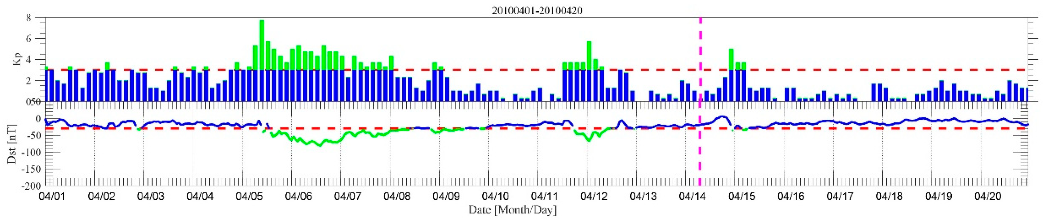
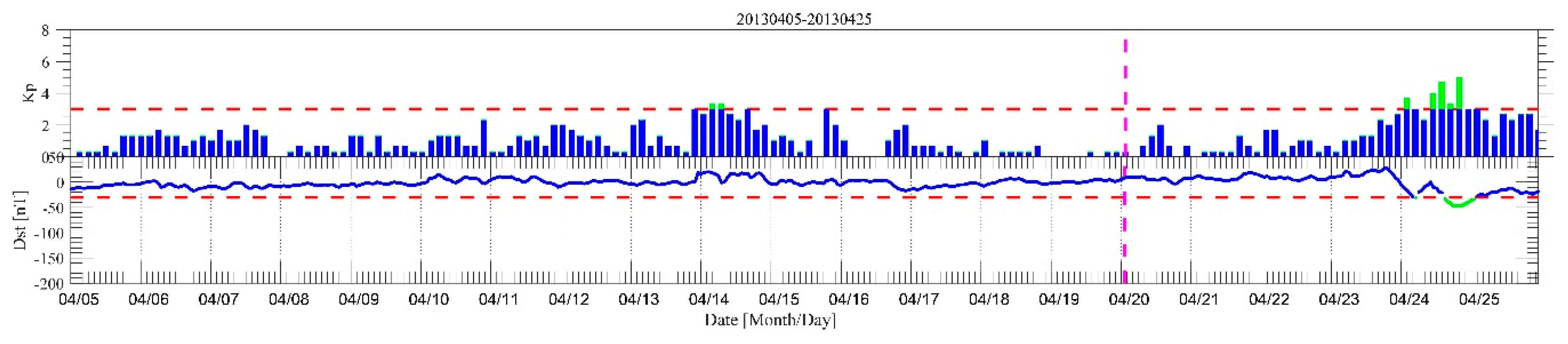
5.1. Other Factors May Induce Disturbance in the Ionosphere

Lightning, geomagnetic storms, solar flares, and other natural sources may induce disturbance in the lower ionosphere [29,47,48,49]. From the index of Dst and Kp (Figure 3), we can see that there were two moderate geomagnetic storms (−100 nT < Dst < −50 nT) before the Yushu earthquake. Generally, moderate storms are highly unlikely to affect the D region of the ionosphere [29,49]. A study by Kumar and Kumar [46] on geomagnetic storm effects demonstrated that a storm with Dst < −140 nT has no effect on VLF signals. In this research, the minimum Dst during geomagnetic storms is −80 nT, which means that this storm is highly unlikely to affect the D region of the ionosphere. We also use COSMIC data to obtain the electron density in the lower ionosphere; the results show no obvious anomalies in the lower ionosphere on the nighttime of 7 April. Furthermore, we also conducted nighttime fluctuation analysis excluding data during geomagnetic storms (6–7 April and 12 April 2010). The results show that an anomaly occurred on 8 April (see Supplementary Figure S3). Thus indicates that possible seismic anomalies may have started on 6 April and lasted until 8 April 2010. Thus, the above characteristics illustrate that the anomaly of nighttime fluctuation analysis on the Yushu earthquake should be unconcerned with geomagnetic storms. In addition, geomagnetic and space weather activities were very quiet before the Lushan earthquake; the anomalies before the Lushan earthquake should, thus, be unconcerned with geomagnetic storms.
The early/fast events of lightning flashes produce a vertical electric filed, which could be projected to the lower ionosphere and lower its effective reflection height for VLF waves [50]. A lightning flash is very rare in our research region (only four events from February 2010 to April 2010, with almost no events in April 2013 in the detecting path between NOV and Ya’an, which was sourced from the following website (https://lightning.nsstc.nasa.gov/nlisib/nlissearch.pl?coords=?579,18)); thus, the effect of lightning can be ignored in this study.
As is known, solar flare can induce ionospheric D region perturbations that influence the subionospheric VLF/LF propagation as an anomaly in amplitude and/or in phase [5,51]. We checked solar activity from 1–20 April and did not find any X-ray flux burst (http://rwcc.bao.ac.cn/history/index.jsp). Thus, the anomaly detected in this study could not induced by solar activities.

5.2. Simulation of Terminator Time Shift

Many researches have introduced the method of terminator time shift to predict the anomalies of earthquakes. Some researchers have declared that a possible reason is the increase in D region electron density, which lowers the boundary of the ionosphere [33]. The lowering of D region boundary changes the condition for modal interference to result in a shift in the VLF signal minima [29]. We also conducted a simulation to check for this phenomenon. We selected an NWC transmitter with transmitting frequency 19.8 kHz, which has maximum power in the southern hemisphere as the source; the electron density and geomagnetic parameters are obtained at the NWC location (114°E, 22°S). The bottom height of the ionosphere was 65 km during LT 6:00–18:00 corresponding to the daytime, which is 80 km for another time corresponding to the nighttime. The blue solid line in Figure 13 shows the simulated Z component of the electric field 1,350 km from NWC under this IRI profile. We can see that a terminator time exists at LT 5:00 and 19:00, which corresponds to sunrise and sunset, respectively. When we lower the bottom height of the ionosphere from 80 km to 66 km at LT 5:00 and 19:00, the calculated result shows that a sunrise terminator time exists at LT 4:00 (shown as the red solid line with pentagrams in Figure 13), which indicates that the terminator time shift an hour forward. The sunset terminator time exists at LT 20:00 (shown as a red solid line with pentagrams in Figure 13), indicating that the terminator time shift an hour backward. The simulated result demonstrates that the terminator time shift could have been induced by lowering of the boundary of the ionosphere. The reason for this could be modal interference of the VLF wave in the waveguide.

5.3. The Simulated Result at Other Locations

As is known, the amplitude of an electric field at different ground locations will be different, owing to modal interference in the waveguide. Figure 14a,b shows the simulated Ez of the electric field 2400 km and 3000 km away from the NOV transmitter. The intensity of Ez is different at different locations. The terminator time is slightly different because of different modal interferences, but the main characteristics of sunrise and sunset have been shown in the figure. The electric field at these locations could also be disturbed by variation in bottom boundary of the ionosphere at the different locations (the red solid line with pentagrams shown in Figure 14a,b). The red solid line with pentagrams in Figure 14a shows the Ez components increased when the bottom height of the ionosphere descends to 63 km at LT 11:00. The simulated increasing amplitude of the electric field could be possible in a longer propagating path with descending reflection height, which was illustrated by Mcrae and Thomson [51] using observed data from the NLK transmitter to the VLF receiver located at Dunedin. The red solid line with pentagrams in Figure 14b shows the Ez components decrease 3000 km from NOV when the bottom height of the ionosphere descends to 63 km at LT 11:00, compared to the original IRI profile.

6. Conclusions

In this paper, the instruments and data format of ALPHA monitoring stations were detailed. The amplitude of electric field recorded by the stations were investigated to detect precursors to the Ms 7.1 Yushu earthquake on 14 April 2010, and the Ms 7.0 Lushan earthquake on 20 April 2013. A full wave model was used to research the possible factors that could induce seismic anomalies on the received VLF electric field.
(1)
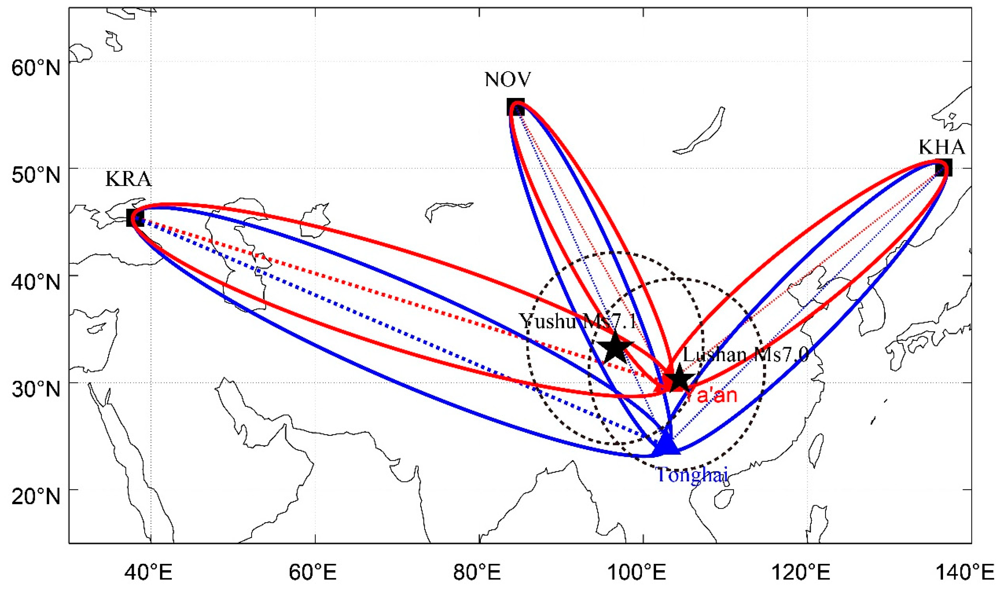
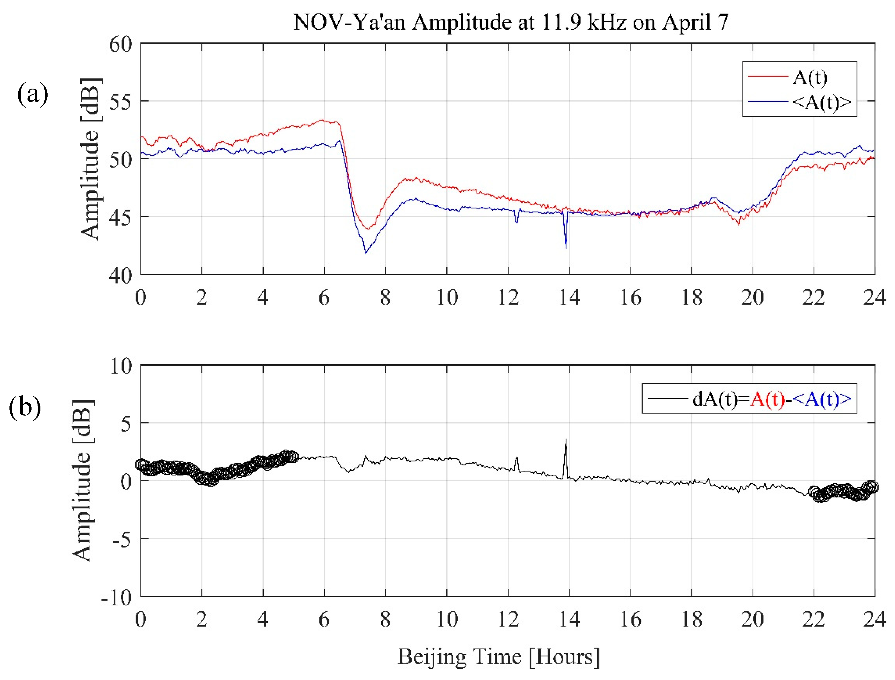
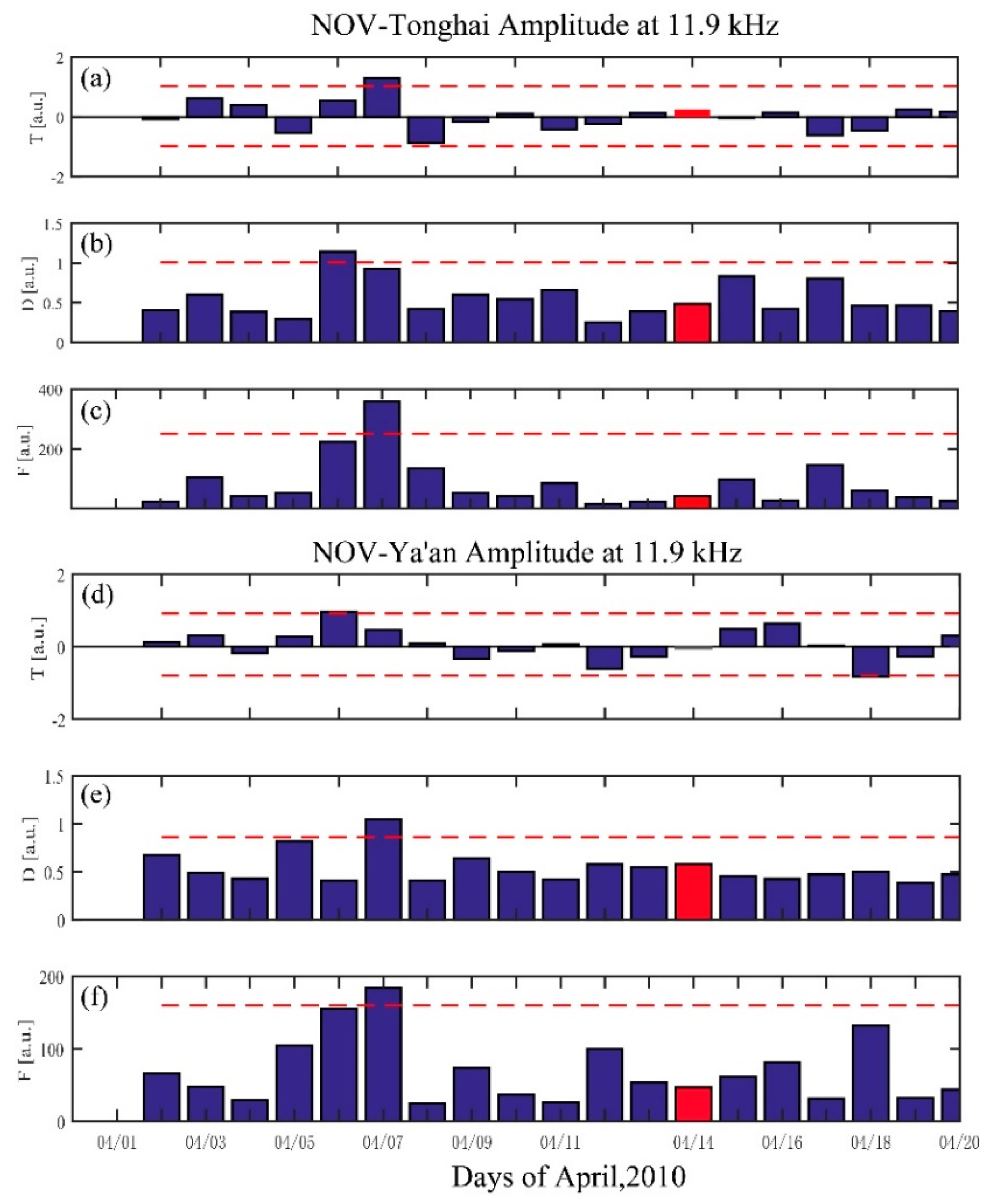
The results of the nighttime fluctuation analysis show that there was an obvious anomaly on 7 April (7 days before the Yushu earthquake) between the transmitter (NOV) and the receivers (Ya’an, Tonghai).
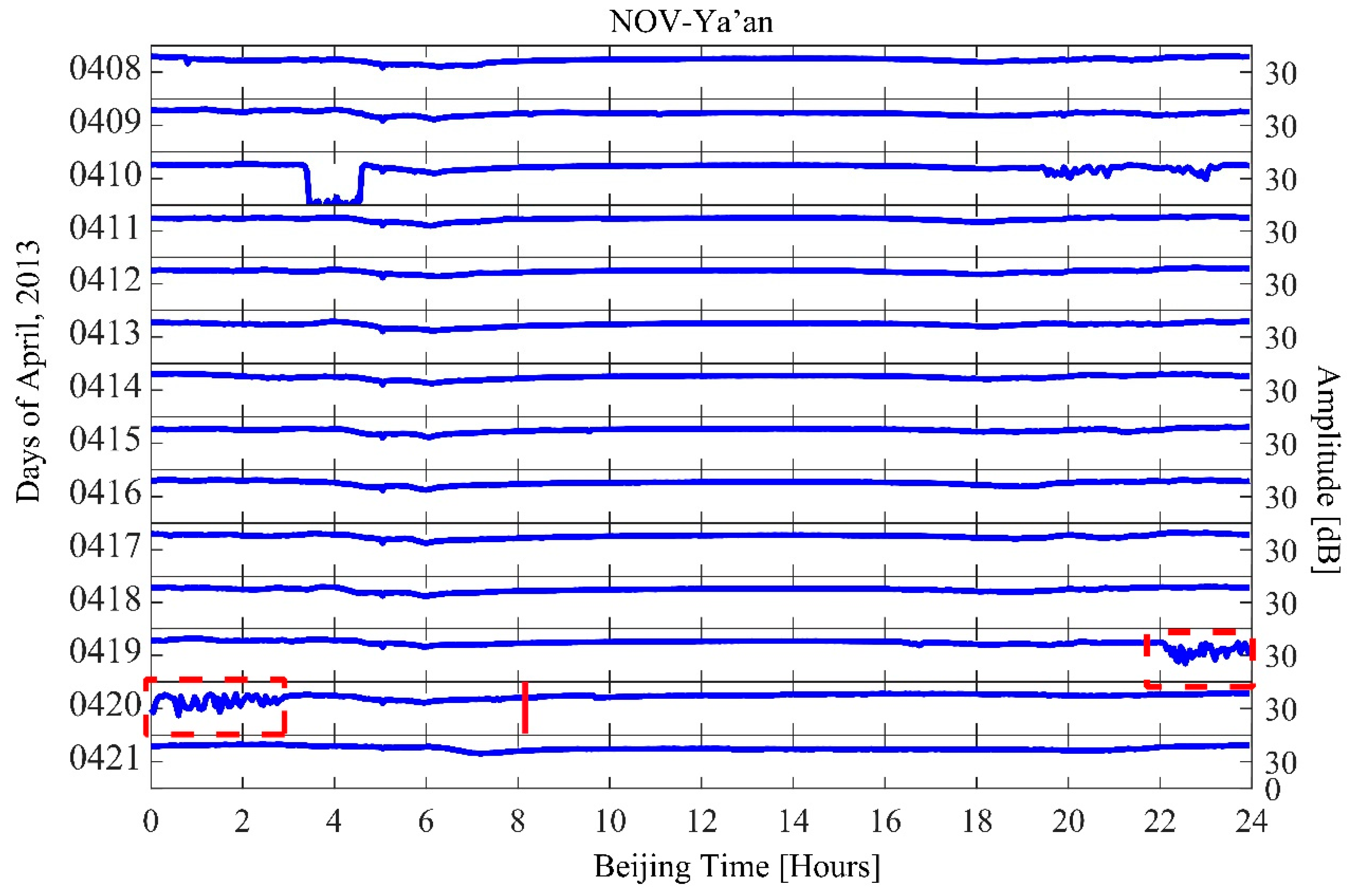
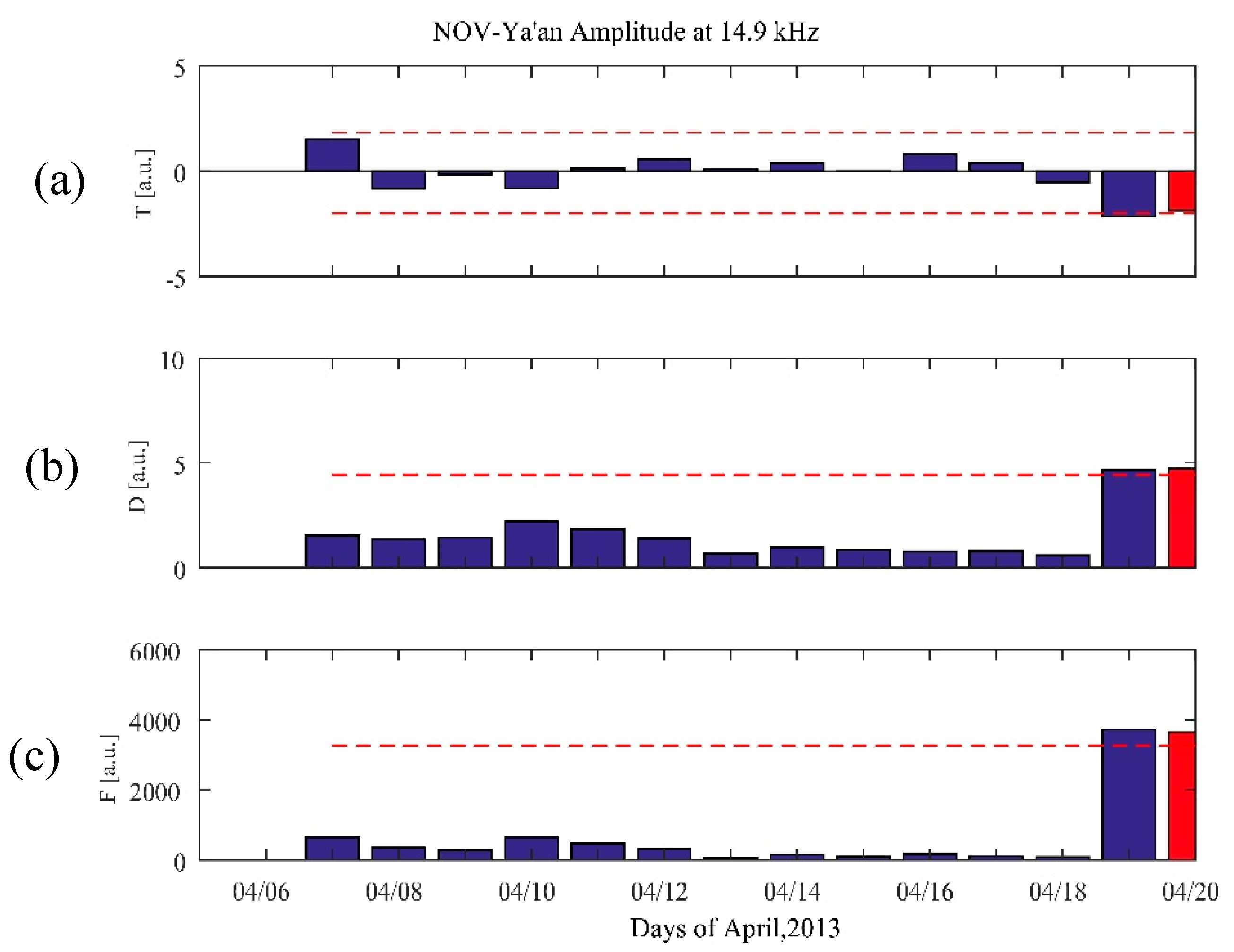
(2)
The results of the nighttime fluctuation analysis show that there was a remarkable anomaly on the night of 19 April and before dawn of 20 April (1 days before the Lushan earthquake) between the transmitter (NOV) and the receivers (Ya’an).
(3)
The anomaly is much more significant for the Lushan earthquake, which may be attributed to the VLF receiver being much closer to the epicenter of the earthquake.
(4)
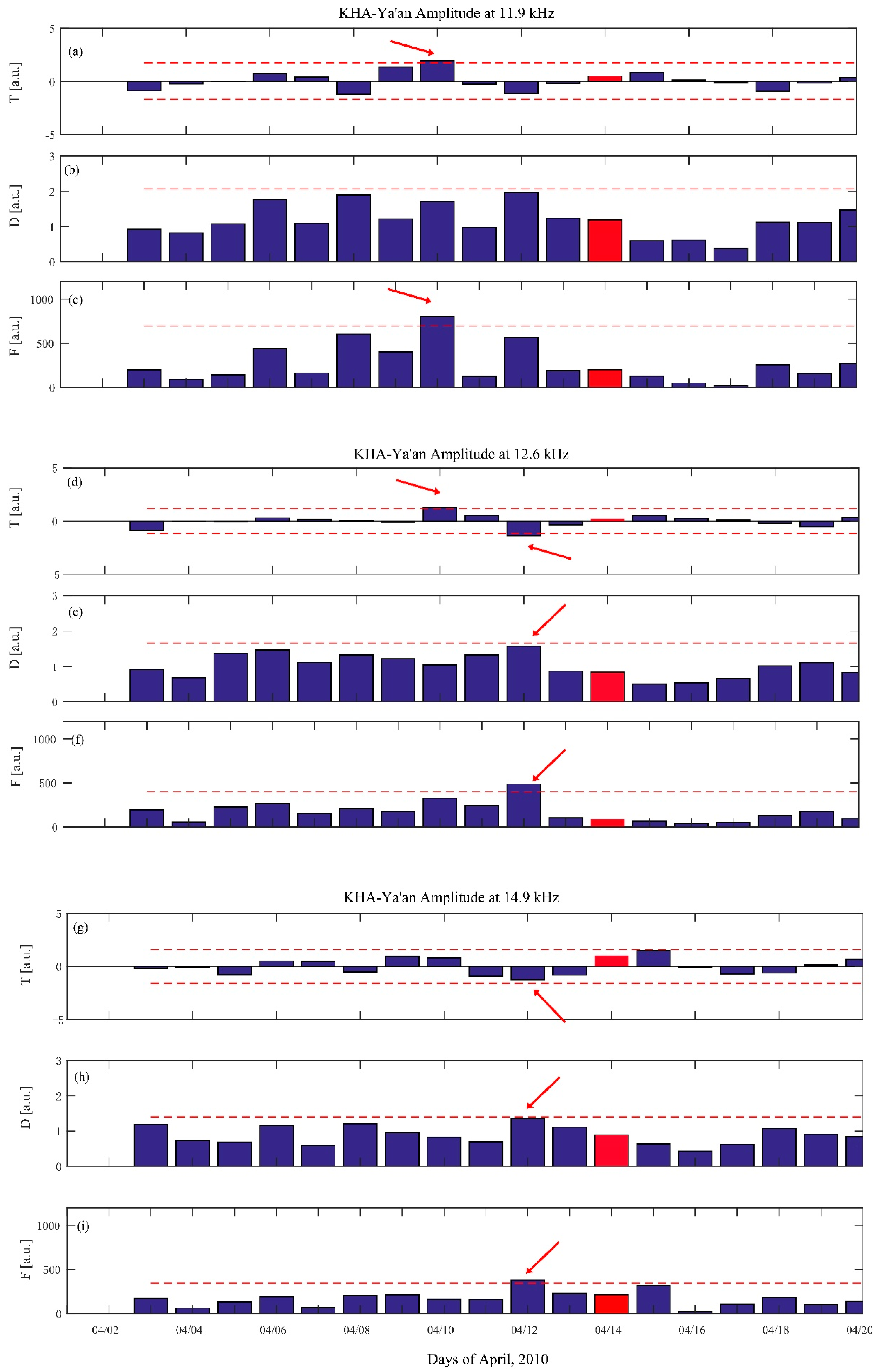
The results of the nighttime fluctuation analysis also show two obvious anomalies on 10 April (4 days before Yushu earthquake) and 12 April (2 days before Yushu earthquake) between the transmitter (KHA) and the receivers (Ya’an).
(5)
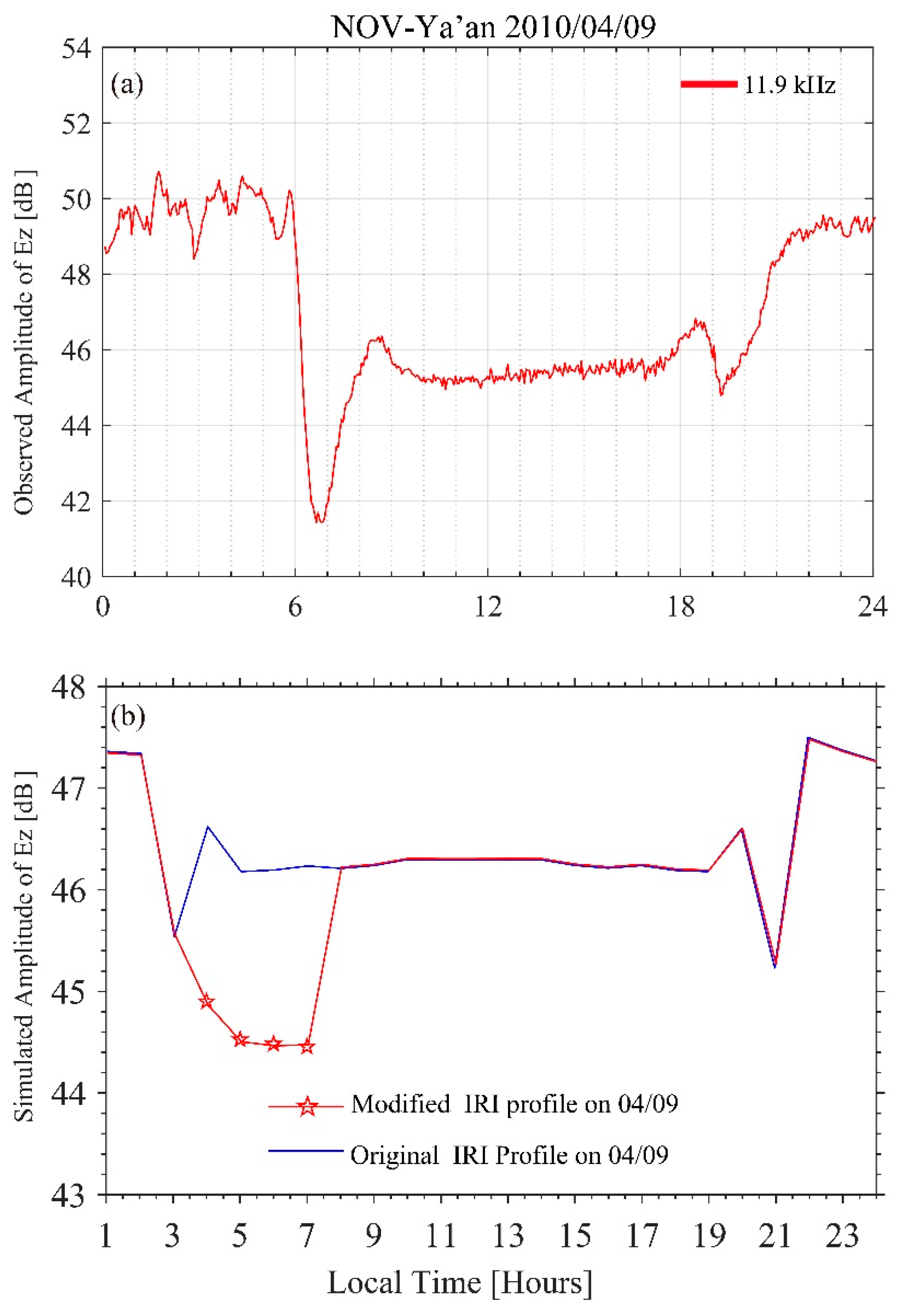
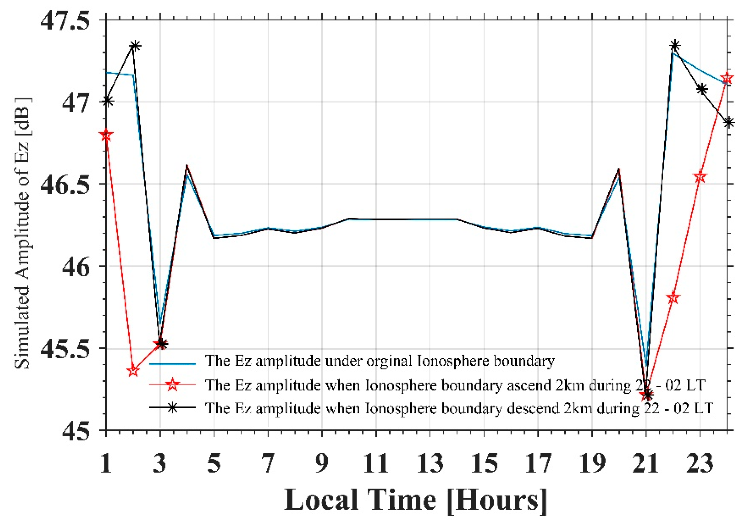
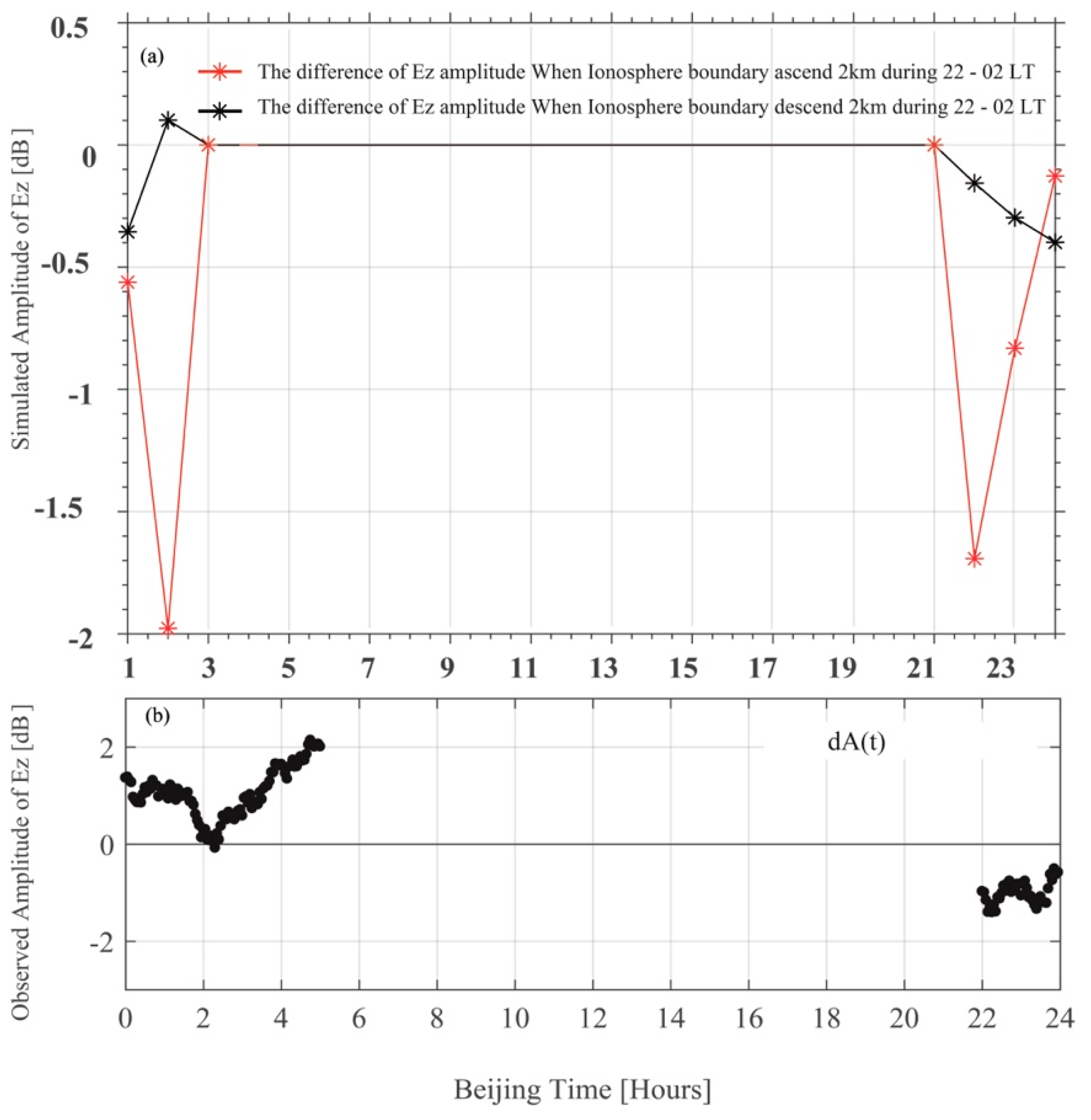
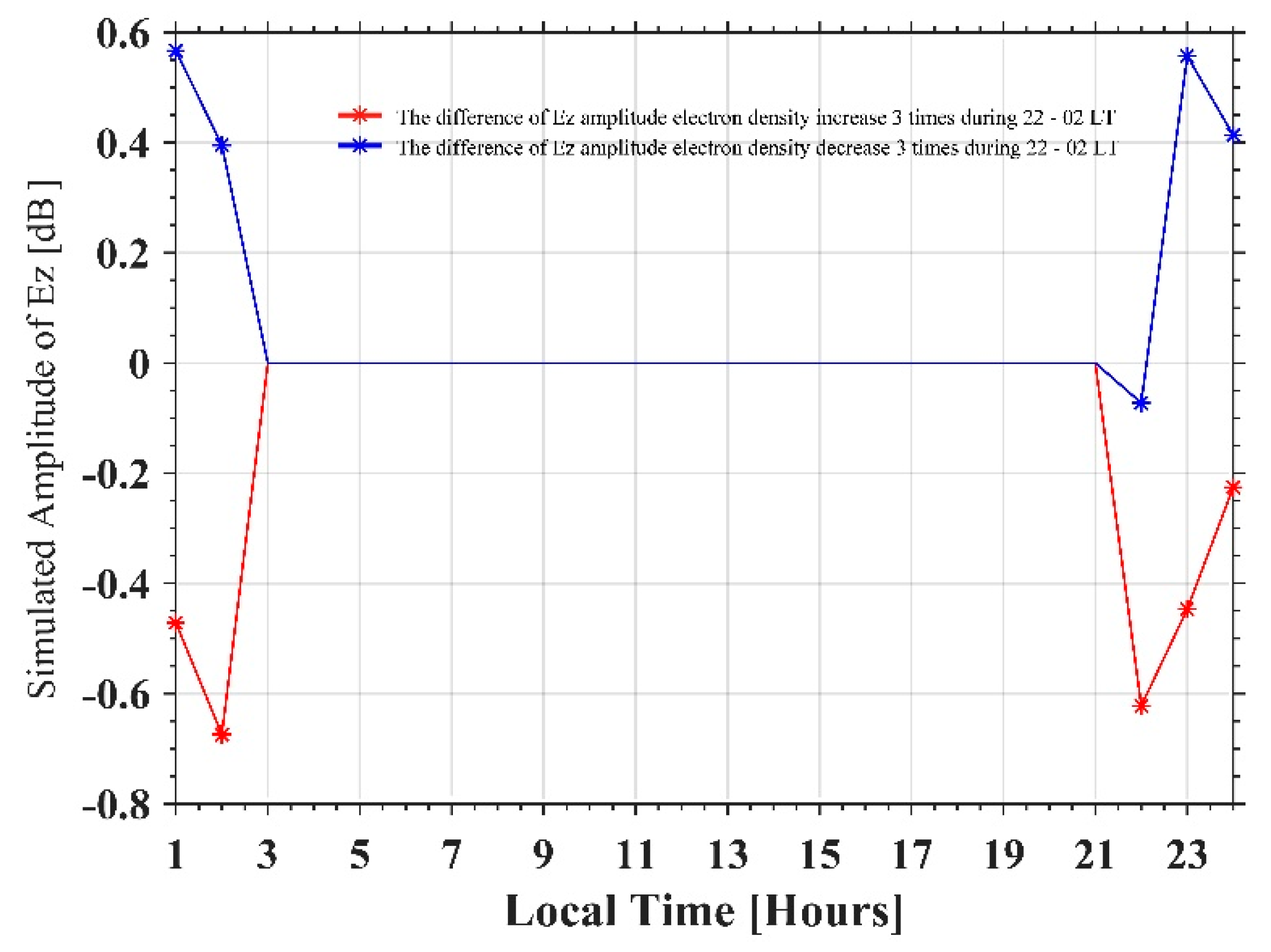
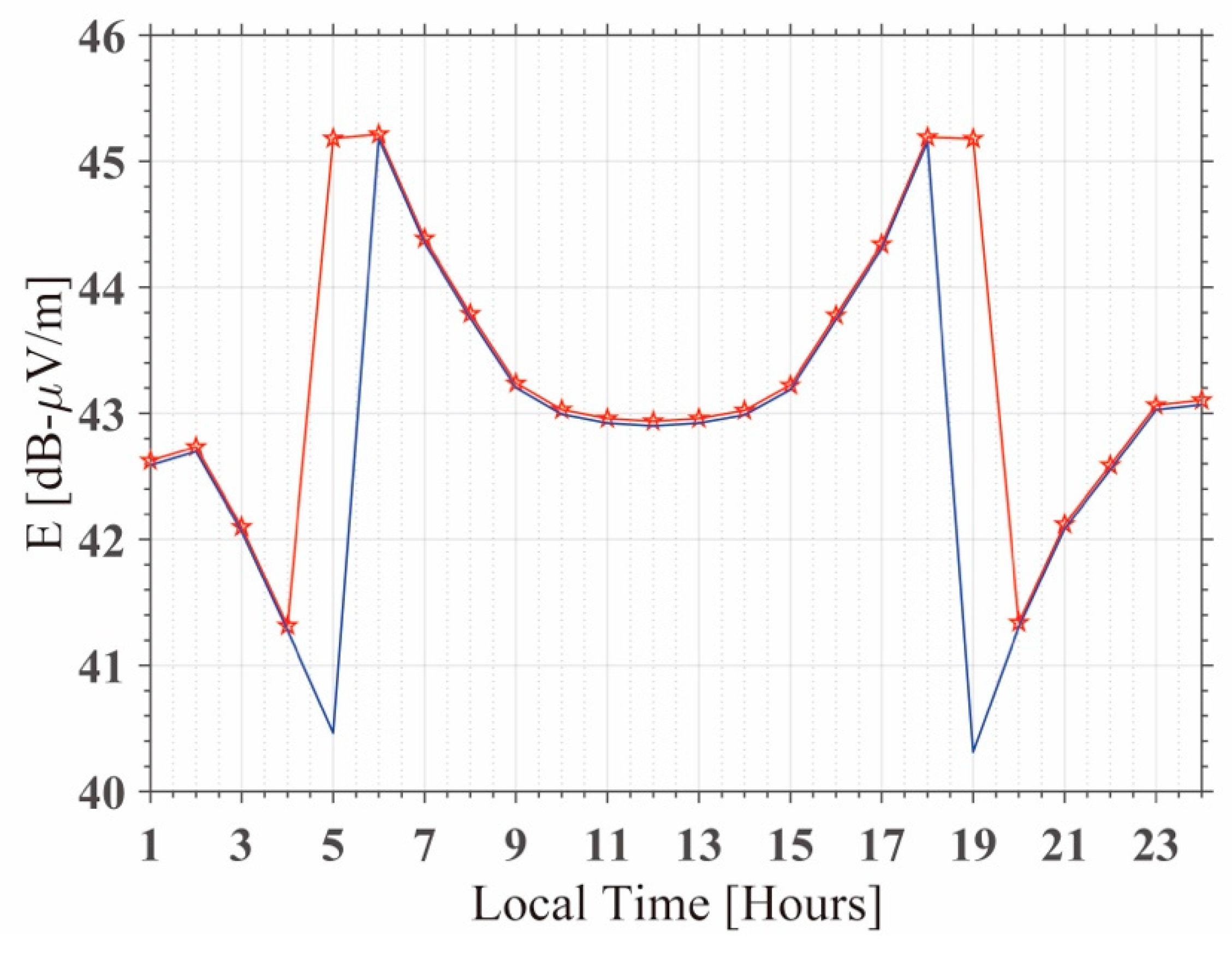
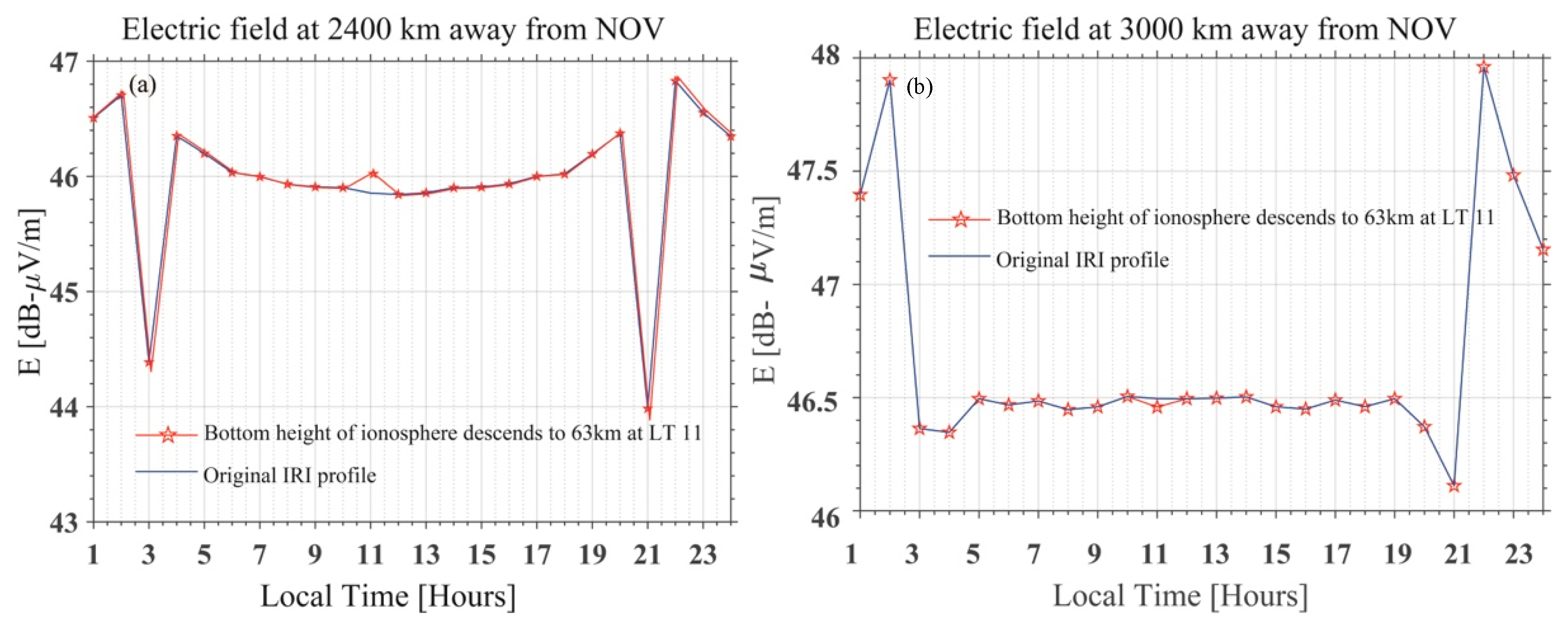
The simulated result illustrates that the received electric field from the VLF transmitters could change abnormally because of variation in bottom boundary of the ionosphere or variation in electron density in the ionosphere. However, the change induced by variation in bottom boundary of the ionosphere is remarkable. The same conclusion was obtained from the simulated results at different locations of ground receivers.
(6)
Combining the observation and simulation, we conclude that the more plausible explanation is that the anomalies are induced by a depletion in D region caused by seismogenic activity, which lowers the effective height of the ionosphere in this event.
(7)
Our simulation has demonstrated that terminator time shift could be induced by the descending of the bottom boundary of the ionosphere, which is due to the modal interference between different modes.
In this study, based on the analysis of sub-ionospheric VLF signals, the possible precursor activity of two strong earthquakes that occurred in western China (Yushu earthquake and Lushan earthquake) has been found. The difference in effective detection range determined by different detecting paths and different frequency signals may provide the basis for identifying the location of the ionospheric disturbance of the earthquake, which should be studied in detail in future. The full wave model was used to provide possible explanations into precursors that occurred prior to the Yushu and Lushan earthquakes.

Supplementary Materials

The following are available online at https://www.mdpi.com/2072-4292/12/21/3563/s1, Figure S1: The observed Ez amplitude in the path between NOV and Ya’an on 5 April, Figure S2: Nighttime Fluctuations analysis for April 2010 for the Yushu earthquake on 14 April 2010 at the path between NOV-Tonghai and Ya’an at F2 and F3. Figure S3: Nighttime Fluctuations analysis for April 2010 for the Yushu earthquake on 14 April 2010 at the path between NOV-Tonghai and Ya’an when excluded the data on 6, 7, 12 April.

Author Contributions

Conceptualization, S.Z. L.L.; Formal analysis, S.Z.; Investigation, S.Z.; Methodology, S.Z., Z.Z., and X.S.; Resources, S.Z., X.S., Z.W., and Z.Z.; Supervision, S.Z. X.S.; Visualization, S.Z.; Writing-original draft, S.Z. L.L.; Writing-review & editing, S.Z., L.L., Z.Z., C.Z., J.C. H.L. and X.S. All authors have read and agreed to the published version of the manuscript.

Funding

This work is supported by the National Natural Science Foundation of China (grants 41704156 41874174); National Key R&D Program of China (grant 2018YFC1503501); Research Grant from National Institute of Natural Hazards, Ministry of Emergency Management of China (Grant no. ZDJ2018-18 and ZDJ2020-06); Research grant from China Research Institute of Radiowave Propagation (Research on low ionosphere satellite detection) and the APSCO Earthquake Research Project Phase II.

Acknowledgments

We acknowledge the DEMETER scientific mission center for providing data of DEMETER satellite (http://demeter.cnrs-orleans.fr). The COSMIC, Dst and Kp index data can be obtained from the website https://cdaac-www.cosmic.ucar.edu/cdaac/cgi_bin/fileFormats.cgi?type=ionPrf; http://wdc.kugi.kyoto-u.ac.jp/dst_final/index.html; ftp://ftp.gfz-potsdam.de/pub/home/obs/kp-ap/wdc/yearly/ respectively.

Conflicts of Interest

The authors declare that they have no competing interests.

References

  1. Budden, K.G. Radio Waves in the Ionosphere; Cambridge University Press: Cambridge, UK, 2009. [Google Scholar]
  2. Cummer, S.A.; Inan, U.S.; Bell, T.F. Ionospheric D region remote sensing using VLF radio atmospherics. Radio Sci. 1998, 33, 1781–1792. [Google Scholar] [CrossRef] [Green Version]
  3. Inan, U.S.; Pasko, V.P.; Bell, T.F. Sustained heating of the ionosphere above thunderstorms as evidenced in “early/fast” VLF events. Geophys. Res. Lett. 1996, 23, 1067–1070. [Google Scholar] [CrossRef]
  4. Kikuchi, T.; Evans, D.S. Quantitative study of substorm-associated VLF phase anomalies and precipitating energetic electrons on November 13, 1979. J. Geophys. Res. Atmos. 1983, 88, 871–880. [Google Scholar] [CrossRef]
  5. Todoroki, Y.; Maekawa, S.; Yamauchi, T.; Horie, T.; Hayakawa, M. Solar flare induced D region perturbation in the ionosphere, as revealed from a short-distance VLF propagation path. Geophys. Res. Lett. 2007, 34, 300–315. [Google Scholar] [CrossRef]
  6. Pulinets, S.A.; Boyarchuk, K.A.; Hegai, V.V.; Kim, V.P.; Lomonosov, A.M. Quasielectrostatic model of atmosphere-thermosphere-ionosphere coupling. Adv. Space Res. 2000, 26, 1209–1218. [Google Scholar] [CrossRef]
  7. Sorokin, V.M.; Chmyrev, V.M.; Yaschenko, A.K. Electrodynamic model of the lower atmosphere and the ionosphere coupling. J. Atmos. Sol. Terr. Phys. 2001, 63, 1681–1691. [Google Scholar] [CrossRef]
  8. Molchanov, O.A. On the origin of low- and middler-latitude ionospheric turbulence. Phys. Chem. Earth Parts A/B/C 2004, 29, 559–567. [Google Scholar] [CrossRef]
  9. Rozhnoi, A.A.; Solovieva, M.S.; Molchanov, O.A.; Chebrov, V.; Voropaev, V.; Hayakawa, M.; Maekawa, S.; Biagi, P.F. Preseismic anomaly of LF signal on the wave path Japan–Kamchatka during November–December 2004. Phys. Chem. Earth Parts A/B/C 2006, 31, 422–427. [Google Scholar] [CrossRef]
  10. Freund, F.; Takeuchi, A.; Lau, B.W.; Post, R.; Keefner, J.W.; Mellon, J.; Almanaseer, A. Stress-Induced Changes in the Electrical Conductivity of Igneous Rocks and the Generation of Ground Currents. Terr. Atmos. Ocean. Sci. 2004, 15, 437–467. [Google Scholar] [CrossRef] [Green Version]
  11. Henderson, T.R.; Sonwalkar, V.S.; Helliwell, R.A.; Inan, U.S.; Frasersmith, A.C. A search for ELF/VLF emissions induced by earthquakes as observed in the ionosphere by the DE 2 satellite. J. Geophys. Res. 1993, 98, 9503–9514. [Google Scholar] [CrossRef]
  12. Parrot, M. Statistical Study Of Elf/Vlf Emissions Recorded by a Low-Altitude Satellite during Seismic Events. J. Geophys. Res. Space Phys. 1994, 99, 23339–23347. [Google Scholar] [CrossRef]
  13. Serebryakova, O.N.; Bilichenko, S.V.; Chmyrev, V.M.; Parrot, M.; Rauch, J.; Lefeuvre, F.; Pokhotelov, O.A. Electromagnetic ELF radiation from earthquake regions as observed by low-altitude satellites. Geophys. Res. Lett. 1992, 19, 91–94. [Google Scholar] [CrossRef]
  14. Yoshida, S.; Uyeshima, M.; Nakatani, M. Electric potential changes associated with slip failure of granite: Preseismic and coseismic signals. J. Geophys. Res. 1997, 102, 14883–14897. [Google Scholar] [CrossRef]
  15. Kuo, C.L.; Huba, J.D.; Joyce, G.; Lee, L.C. Ionosphere plasma bubbles and density variations induced by pre-earthquake rock currents and associated surface charges. J. Geophys. Res. 2011, 116, A10317. [Google Scholar] [CrossRef] [Green Version]
  16. Namgaladze, A.; Klimenko, M.; Klimenko, V.; Zakharenkova, I. Physical mechanism and mathematical modeling of earthquake ionospheric precursors registered in total electron content. Geomagn. Aeron. 2009, 49, 252–262. [Google Scholar] [CrossRef]
  17. Zhou, C.; Liu, Y.; Zhao, S.F.; Liu, J.; Zhang, X.M.; Huang, J.P.; Shen, X.H.; Ni, B.B.; Zhao, Z.Y. An electric field penetration model for seismo-ionospheric research. Adv. Space Res. 2017, 60, 2217–2232. [Google Scholar] [CrossRef]
  18. Liu, J.Y.; Chen, Y.I.; Chen, C.H.; Liu, C.Y.; Chen, C.Y.; Nishihashi, M.; Li, J.Z.; Xia, Y.Q.; Oyama, K.I.; Hattori, K.; et al. Seismoionospheric GPS total electron content anomalies observed before the 12 May 2008 Mw7.9 Wenchuan earthquake. J. Geophys. Res. 2009, 114, A04320. [Google Scholar] [CrossRef]
  19. Liu, J.Y.; Chen, Y.I.; Chuo, Y.J.; Tsai, H.F. Variations of ionospheric total electron content during the Chi-Chi earthquake. Geophys. Res. Lett. 2001, 28, 1383–1386. [Google Scholar] [CrossRef] [Green Version]
  20. Ondoh, T. Anomalous sporadic E ionization before a great earthquake. Adv. Space Res. 2004, 34, 1830–1835. [Google Scholar] [CrossRef]
  21. Yao, Y.B.; Chen, P.; Wu, H.; Zhang, S.; Peng, W.F. Analysis of ionospheric anomalies before the 2011 M-w 9.0 Japan earthquake. Chin. Sci. Bull. 2012, 57, 500–510. [Google Scholar] [CrossRef] [Green Version]
  22. Zhao, B.Q.; Wang, M.; Yu, T.; Wan, W.X.; Lei, J.H.; Liu, L.B.; Ning, B.Q. Is an unusual large enhancement of ionospheric electron density linked with the 2008 great Wenchuan earthquake? J. Geophys. Res. 2008, 113, A11304. [Google Scholar] [CrossRef]
  23. Gokhberg, M.B.; Gufeld, I.L.; Rozhnoy, A.A.; Marenko, V.F.; Yampolsky, V.S.; Ponomarev, E.A. Study of seismic influence on the ionosphere by super long-wave probing of the Earth-ionosphere waveguide. Phys. Earth Planet. Inter. 1989, 57, 64–67. [Google Scholar] [CrossRef]
  24. Kasahara, Y.; Muto, F.; Horie, T.; Yoshida, M.; Hayakawa, M.; Ohta, K.; Rozhnoi, A.; Solovieva, M.; Molchanov, O.A. On the statistical correlation between the ionospheric perturbations as detected by subionospheric VLF/LF propagation anomalies and earthquakes. Nat. Hazards Earth Syst. Sci. 2008, 8, 653–656. [Google Scholar] [CrossRef]
  25. Molchanov, O.A.; Hayakawa, M. Subionospheric VLF signal perturbations possibly related to earthquakes. J. Geophys. Res. Space Phys. 1998, 103, 17489–17504. [Google Scholar] [CrossRef]
  26. Hayakawa, M. VLF/LF Radio Sounding of Ionospheric Perturbations Associated with Earthquakes. Sensors 2007, 7, 1141–1158. [Google Scholar] [CrossRef] [Green Version]
  27. Hayakawa, M. The precursory signature effect of the Kobe earthquake on VLF subionospheric signals. J. Comm. Res. Lab 1996, 43, 169–180. [Google Scholar]
  28. Horie, T.; Maekawa, S.; Yamauchi, T.; Hayakawa, M. A possible effect of ionospheric perturbations associated with the Sumatra earthquake, as revealed from subionospheric very-low-frequency (VLF) propagation (NWC-Japan). Int. J. Remote Sens. 2007, 28, 3133–3139. [Google Scholar] [CrossRef]
  29. Maurya, A.K.; Venkatesham, K.; Tiwari, P.; Vijaykumar, K.; Singh, R.; Singh, A.K.; Ramesh, D.S. The 25 April 2015 Nepal Earthquake: Investigation of precursor in VLF subionospheric signal. J. Geophys. Res. Space Phys. 2016, 121, 10403–10416. [Google Scholar] [CrossRef] [Green Version]
  30. Biagi, P.F.; Piccolo, R.; Ermini, A.; Martellucci, S. Possible earthquake precursors revealed by LF radio signals. Nat. Hazards Earth Syst. Sci. 2001, 1, 99–104. [Google Scholar] [CrossRef] [Green Version]
  31. Shvets, A.V. Results of subionospheric radio LF monitoring prior to the Tokachi (M=8, Hokkaido, 25 September 2003) earthquake. Nat. Hazards Earth Syst. Sci. 2004, 4, 647–653. [Google Scholar] [CrossRef] [Green Version]
  32. Molchanov, O.A.; Rozhnoi, A.; Solovieva, M.; Akentieva, O.; Berthelier, J.J.; Parrot, M.; Lefeuvre, F.; Biagi, P.F.; Castellana, L.; Hayakawa, M. Global diagnostics of the ionospheric perturbations related to the seismic activity using the VLF radio signals collected on the DEMETER satellite. Nat. Hazards Earth Syst. Sci. 2006, 6, 745–753. [Google Scholar] [CrossRef]
  33. Yoshida, M.; Yamauchi, T.; Horie, T.; Hayakawa, M. On the generation mechanism of terminator times in subionospheric VLF/LF propagation and its possible application to seismogenic effects. Nat. Hazards Earth Syst. Sci. 2008, 8, 332–338. [Google Scholar] [CrossRef] [Green Version]
  34. Lehtinen, N.G.; Inan, U.S. Radiation of ELF/VLF waves by harmonically varying currents into a stratified ionosphere with application to radiation by a modulated electrojet. J. Geophys. Res. 2008, 113, A06301. [Google Scholar] [CrossRef] [Green Version]
  35. Cohen, M.B.; Lehtinen, N.G.; Inan, U.S. Models of ionospheric VLF absorption of powerful ground based transmitters. Geophys. Res. Lett. 2012, 39, L24101. [Google Scholar] [CrossRef] [Green Version]
  36. Lehtinen, N.G.; Inan, U.S. Full-wave modeling of transionospheric propagation of VLF waves. Geophys. Res. Lett. 2009, 36, L03104. [Google Scholar] [CrossRef] [Green Version]
  37. Zhao, S.F.; Zhou, C.; Shen, X.H.; Zhima, Z. Investigation of VLF transmitter signals in the ionosphere by ZH-1 observations and full-wave simulation. J. Geophys. Res. Space Phys. 2019, 124, 4697–4709. [Google Scholar] [CrossRef]
  38. Shen, X.; Zhima, Z.; Zhao, S.; Qian, G.; Ye, Q.; Ruzhin, Y. VLF radio wave anomalies associated with the 2010 Ms 7.1 Yushu earthquake. Adv. Space Res. 2017, 59, 2636–2644. [Google Scholar] [CrossRef]
  39. Yao, L.; Chen, H.; He, Y. The signal to noise ratio disturbance of ionospheric VLF radio signal before the 2010 Yushu Ms7.1 earthquake. Acta Seismol. Sin. 2013, 35, 390–399. [Google Scholar]
  40. Dobrovolsky, I.P.; Zubkov, S.I.; Miachkin, V.I. Estimation of the size of earthquake preparation zones. Pure Appl. Geophys. 1979, 117, 1025–1044. [Google Scholar] [CrossRef]
  41. Molchanov, O.A.; Hayakawa, M. Seismo-Electromagnetics and Related Phenomena: History and Latest Results; TERRAPUB: Tokoy, Japen, 2008. [Google Scholar]
  42. Yeh, K.C.; Liu, C.H. Theory of Ionospheric Waves; Academic Press: New York, NY, USA, 1972. [Google Scholar]
  43. Bilitza, D.; Altadill, D.; Truhlik, V.; Shubin, V.; Galkin, I.; Reinisch, B.; Huang, X. International Reference Ionosphere 2016: From ionospheric climate to real-time weather predictions. Space Weather Int. J. Res. Appl. 2017, 15, 418–429. [Google Scholar] [CrossRef]
  44. Finlay, C.C.; Maus, S.; Beggan, C.D.; Bondar, T.N.; Chambodut, A.; Chernova, T.A.; Chulliat, A.; Golovkov, V.P.; Hamilton, B.; Hamoudi, M.; et al. International Geomagnetic Reference Field: The eleventh generation. Geophys. J. Int. 2010, 183, 1216–1230. [Google Scholar]
  45. Budden, K. The Propagation of Radio Waves: The Theory of Radio Waves of Low Power in the Ionosphere and Magnetosphere; Cambridge University Press: Cambridge, UK, 1985. [Google Scholar]
  46. Marshall, R.A.; Inan, U.S.; Glukhov, V.S. Elves and associated electron density changes due to cloud-to-ground and in-cloud lightning discharges. J. Geophys. Res. 2010, 115, A00E17. [Google Scholar] [CrossRef]
  47. Peter, W.B.; Chevalier, M.W.; Inan, U.S. Perturbations of midlatitude subionospheric VLF signals associated with lower ionospheric disturbances during major geomagnetic storms. J. Geophys. Res. 2006, 111, A03301. [Google Scholar] [CrossRef]
  48. Zigman, V.; Grubor, D.; Sulic, D. D-region electron density evaluated from VLF amplitude time delay during X-ray solar flares. J. Atmos. Sol. Terr. Phys. 2007, 69, 775–792. [Google Scholar] [CrossRef]
  49. Kumar, A.; Kumar, S. Space weather effects on the low latitude D-region ionosphere during solar minimum. Earth Planets Space 2014, 66, 76. [Google Scholar] [CrossRef] [Green Version]
  50. Inan, U.S.; Bell, T.F.; Rodriguez, J.V. Heating and ionization of the lower ionosphere by lightning. Geophys. Res. Lett. 1991, 18, 705–708. [Google Scholar] [CrossRef]
  51. Mcrae, W.M.; Thomson, N.R. Solar flare induced ionospheric D-region enhancements from VLF phase and amplitude observations. J. Atmos. Sol. Terr. Phys. 2004, 66, 77–87. [Google Scholar] [CrossRef]
Figure 1. A sketch of the observation region. The three VLF transmitters in Russia denoted by black square, three receivers in China denoted by triangles (red for Ya’an, blue for Tonghai), the black pentagram represents the epicenter of the Yushu earthquake and the Lushan earthquake, the black dashed circle represents the preparation zone of the Yushu earthquake. The red and blue ellipse denotes the 5th fifth Fresnel region of frequency F1 (11.9 kHz).
Remotesensing 12 03563 g001
Figure 2. (a) The A(t) represents current Ez amplitude between NOV and Ya’an on 7 April, the <A(t)> represents the average Ez amplitude of background (3 days). (b) shows the difference of Ez amplitude of A(t) and <A(t)> on 7 April, the black circles mark the selected nighttime data.
Remotesensing 12 03563 g002
Figure 3. Nighttime fluctuation analysis around the Yushu earthquake on 14 April 2010 in red. The trend (T) (a,d), dispersion (D) (b,e), and fluctuation (F) (c,f) between NOV-Tonghai and Ya’an at F1 are shown separately. The horizontal line in each panel depicts the 2σ deviation criterion to define the anomalous day.
Remotesensing 12 03563 g003
Figure 4. The Kp and Dst index during 1–20 April; the green histogram and curve indicate high geomagnetic activities and space weather activities and the pink dashed line denotes the original time of the Yushu earthquake.
Remotesensing 12 03563 g004
Figure 5. Nighttime fluctuation analysis of KHA-Ya’an at F1, F2, and F3 around the Yushu earthquake on 14 April 2010, shown in red. The trend (T) (a,d,g), dispersion (D) (b,e,h), and fluctuation (F) (c,f,i) of the three frequencies are shown separately. The horizontal line in each panel depicts the 2σ deviation criterion to define the anomalous day; the red arrows mark the anomaly.
Remotesensing 12 03563 g005
Figure 6. The continuous amplitude of Ez (vertical component of electric field) observed during 8 April–21 April; the red rectangular box denotes the night time fluctuation and the red vertical bar represents the time of the Lushan earthquake.
Remotesensing 12 03563 g006
Figure 7. Nighttime fluctuation analysis for the Lushan earthquake on 20 April 2013 is shown in red. The trend (T) (a), dispersion (D) (b), and fluctuation (F) (c) between NOV and Ya’an at F3 are shown separately. The horizontal line in each panel depicts the 2σ deviation criterion that defines the anomalous day.
Remotesensing 12 03563 g007
Figure 8. The Kp and Dst index during 5–25 April 2013; the green histogram and curve indicate high geomagnetic activities and space weather activities, and the pink dashed line denotes the actual time of the Lushan earthquake.
Remotesensing 12 03563 g008
Figure 9. The top panel (a) represents the continuous amplitude of Ez (vertical component of electric field) observed on 9 April. The bottom panel (b) shows the calculated Ez 2700 km away from the NOV transmitter. In (b), the blue solid line shows the calculated Ez under the original IRI profile on 9 April, when sunrise was LT 4:00; the red solid line with pentagrams shows the calculated Ez under the modified IRI profile, when the sunrise time shifted to LT 7:00.
Remotesensing 12 03563 g009
Figure 10. The simulated Ez amplitude under three different bottom heights of ionosphere during 22-02 LT. The blue solid line represents the Ez amplitude under the original IRI profile (bottom height of the ionosphere is 80 km), the red solid line with pentagrams represents the Ez amplitude when the bottom height of the ionosphere ascends to 82 km, the blue solid line with asterisks represents the Ez amplitude when the bottom height of the ionosphere descends to 78 km.
Remotesensing 12 03563 g010
Figure 11. (a) The red solid line with asterisks represents the difference in Ez amplitude when the bottom height of the ionosphere is 82 and 80 km, the black solid line with asterisks represents the difference in Ez amplitude when the bottom height of the ionosphere is 78 and 80 km. (b) shows the difference in Ez components between 7 April (A(t)) and the running mean(<A(t)>). The black circles mark the selected nighttime data.
Remotesensing 12 03563 g011
Figure 12. The red solid line with asterisks represents the difference in Ez amplitude between the electron density (from 100 km to F2 region) set thrice and the original IRI profile. The blue solid line with asterisks represents the difference in Ez amplitude when electron density (from 100 km to F2 region) is set as 1/3 times and the original IRI profile.
Remotesensing 12 03563 g012
Figure 13. The calculated Ez component of the electric field 1,350 km away from the NWC transmitter with 19.8 kHz. The blue solid line shows the simulated result when the sunrise time was set at LT 5:00 and sunset was at LT 19:00. The red solid line with pentagrams shows the simulated result when the sunrise time was set at LT 4:00 and the sunset time was at LT 20:00.
Remotesensing 12 03563 g013
Figure 14. The figure shows the calculated Ez component of the electric field 2400 km (a) and 3000 km (b) from the NOV transmitter at 11.9 kHz. In (a), the blue solid line shows the simulated result under the original IRI profile; the red solid line with pentagrams shows the simulated result when the bottom height of the ionosphere descends at LT 11:00 2400 km from the NOV transmitter. In (b), the blue solid line shows the simulated result under the original IRI profile; the red solid line with pentagrams shows the simulated result when the bottom height of the ionosphere ascends at LT 11:00 3000 km from the NOV transmitter.
Remotesensing 12 03563 g014
Publisher’s Note: MDPI stays neutral with regard to jurisdictional claims in published maps and institutional affiliations.

