Postfire Tree Structure from High-Resolution LiDAR and RBR Sentinel 2A Fire Severity Metrics in a Pinus halepensis-Dominated Burned Stand


Abstract
:
1. Introduction
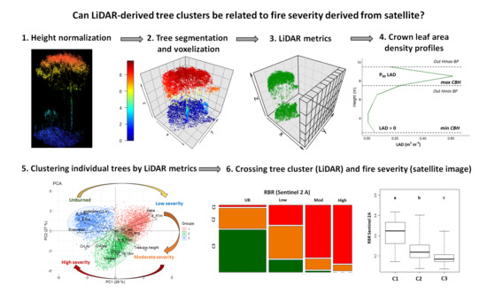
2. Methods
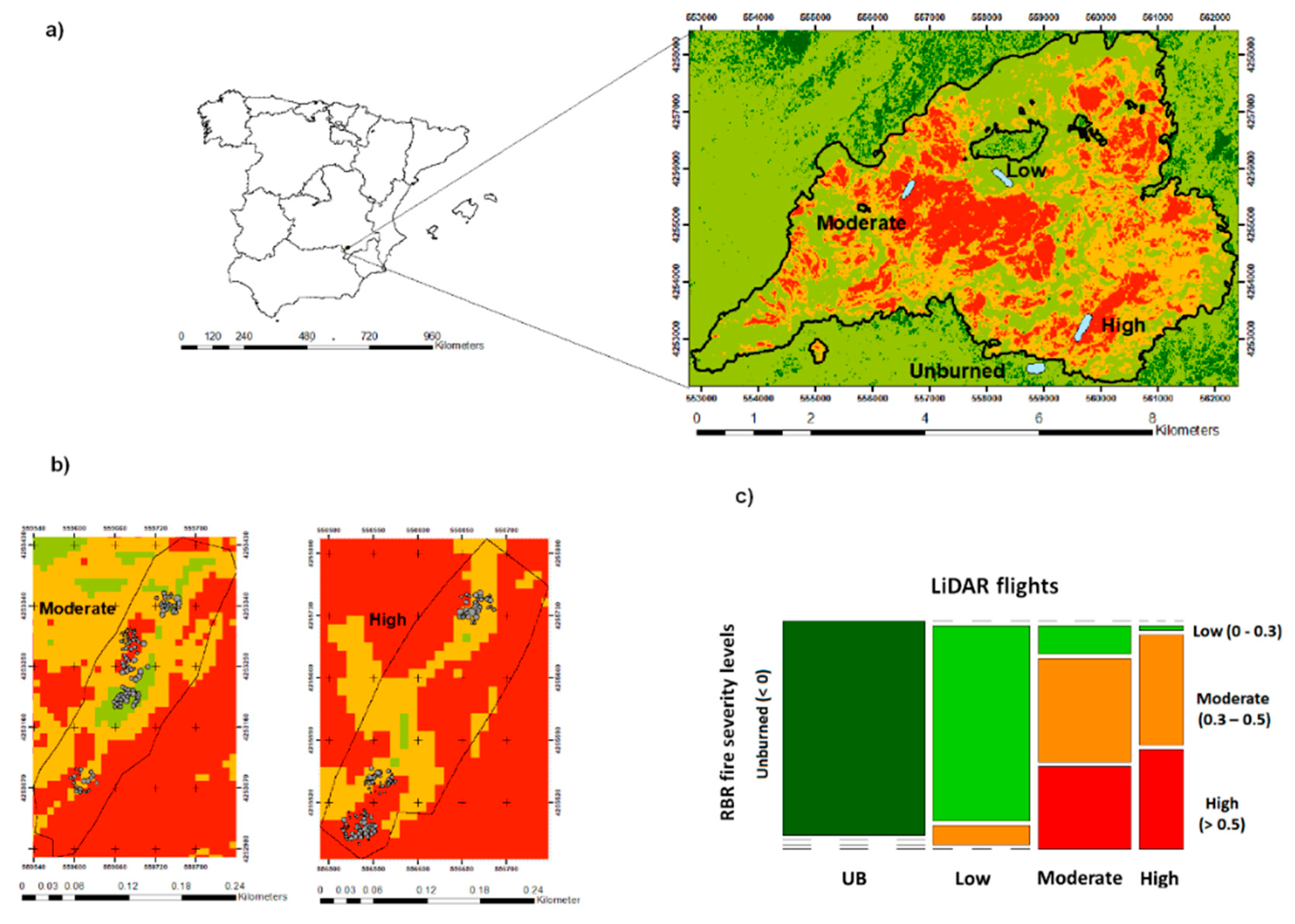
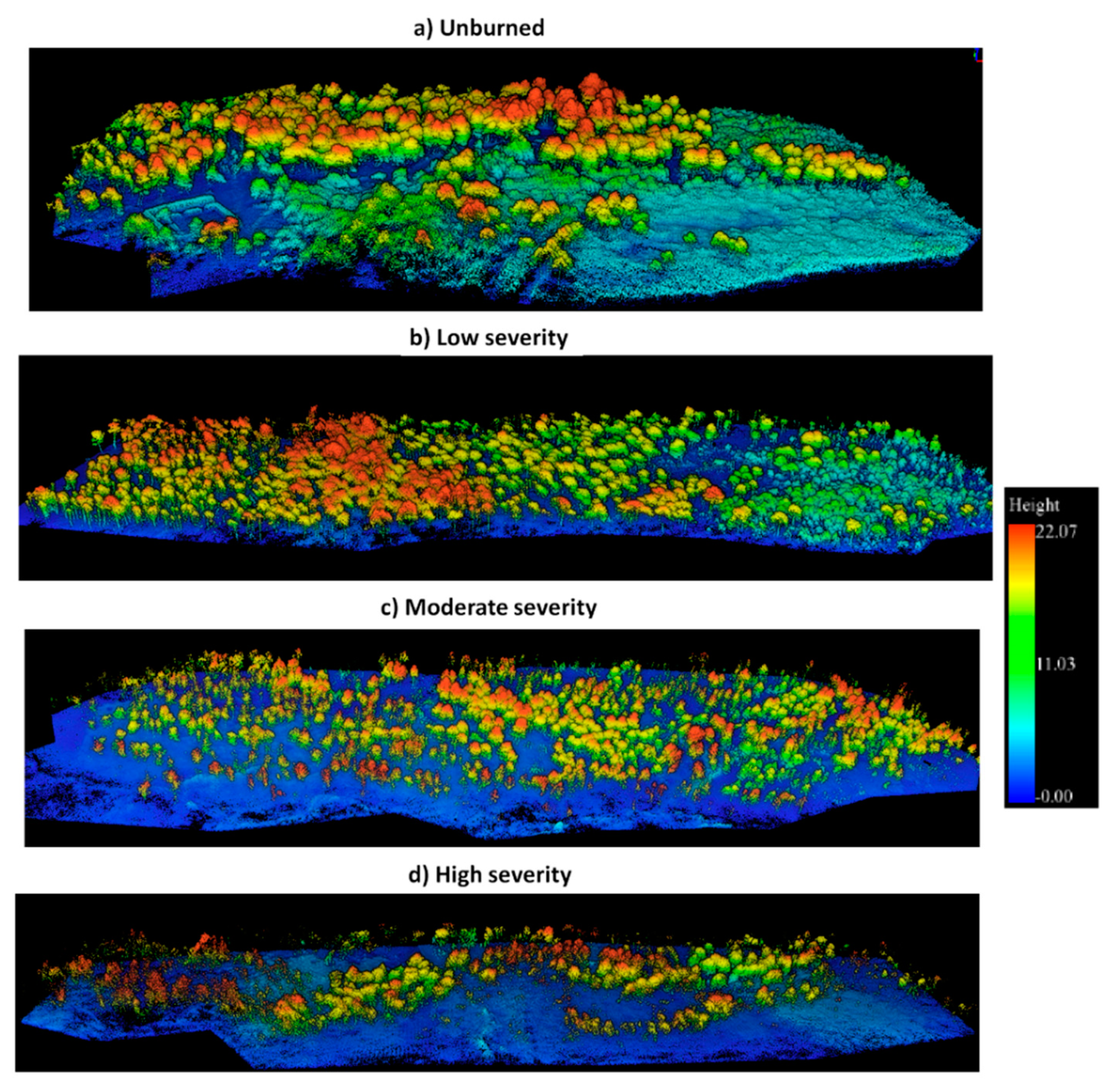
2.1. Study Sites
2.2. LiDAR Data
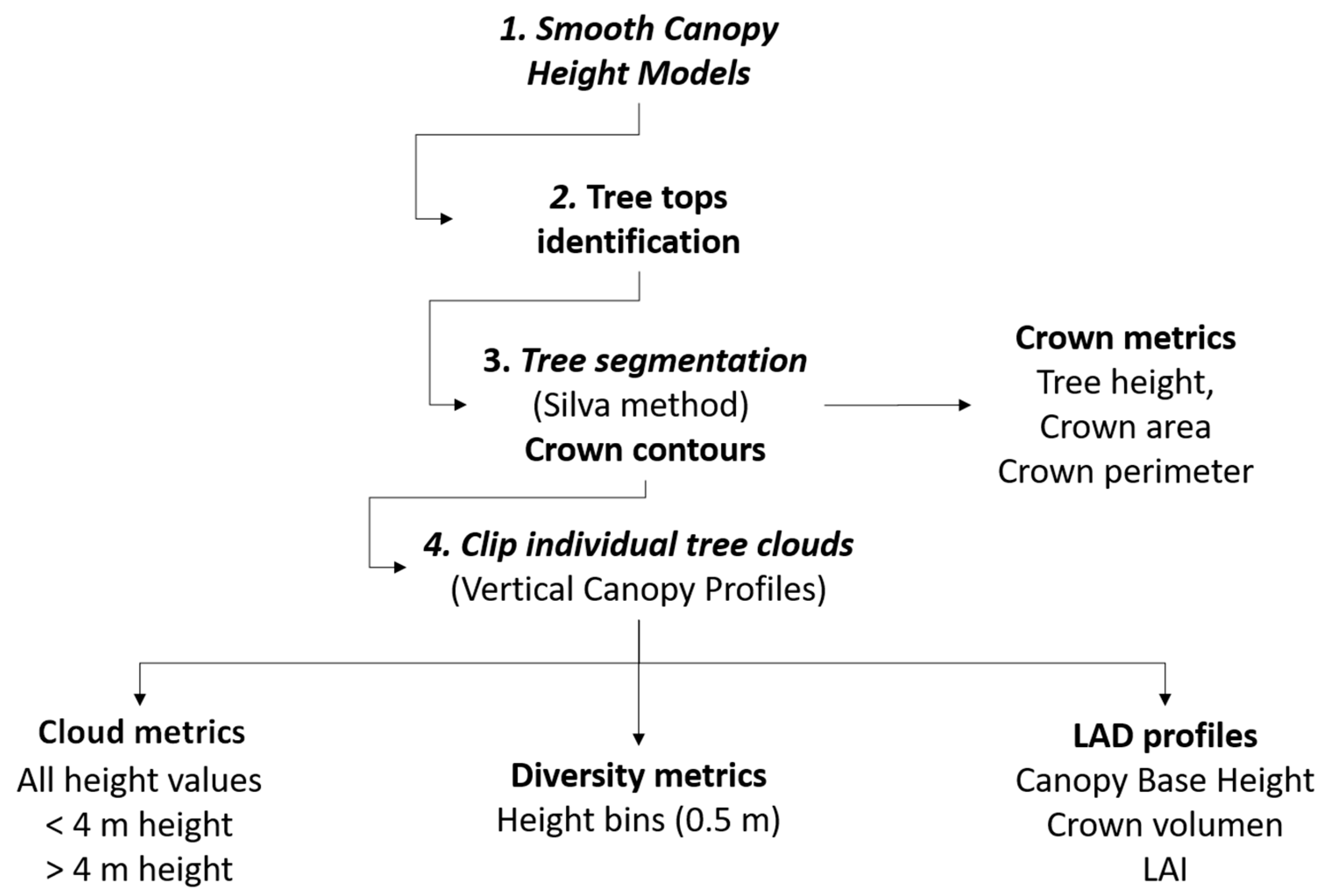
2.2.1. LiDAR Pre-Processing
2.2.2. Tree Detection and Vertical Canopy Profiles (VCP)
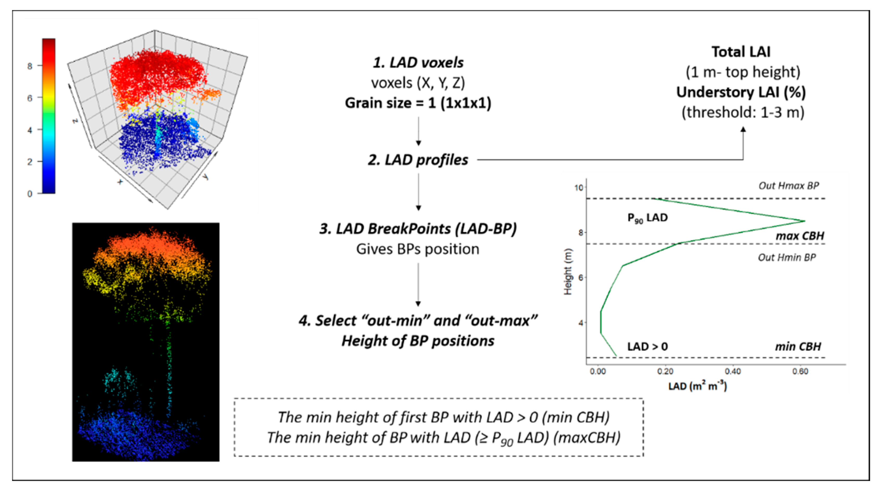
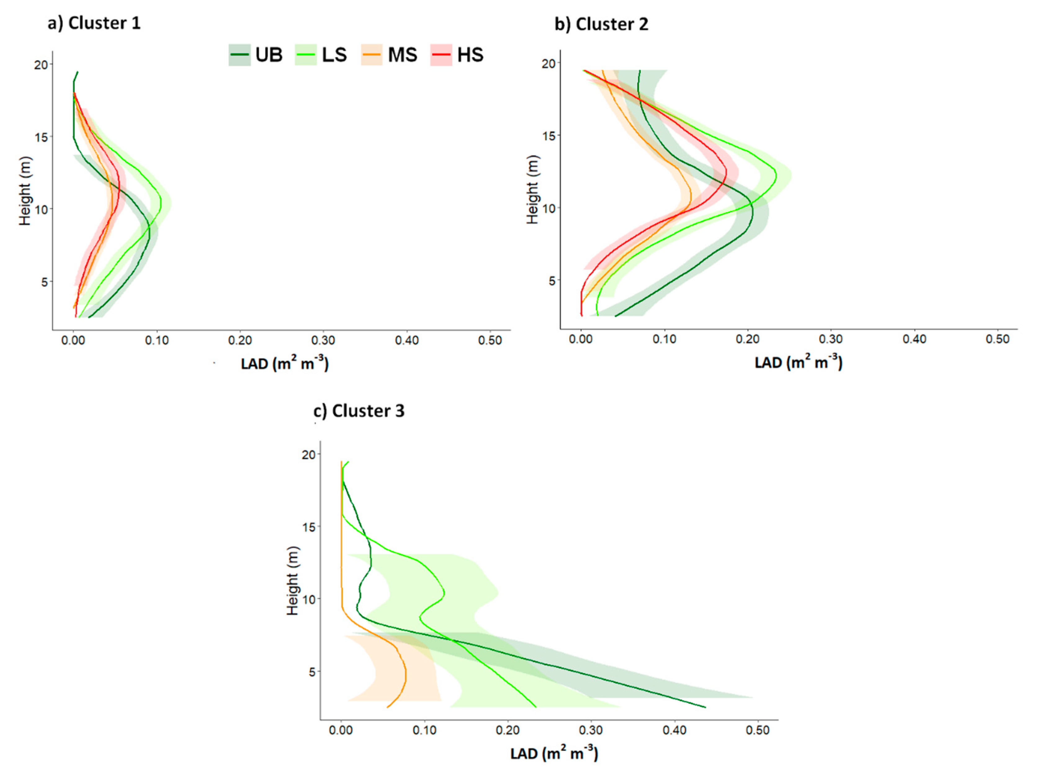
2.2.3. LAI and LAD Profiles
2.3. RBR Sentinel 2 Fire Severity Index
2.4. Statistical Analysis
3. Results
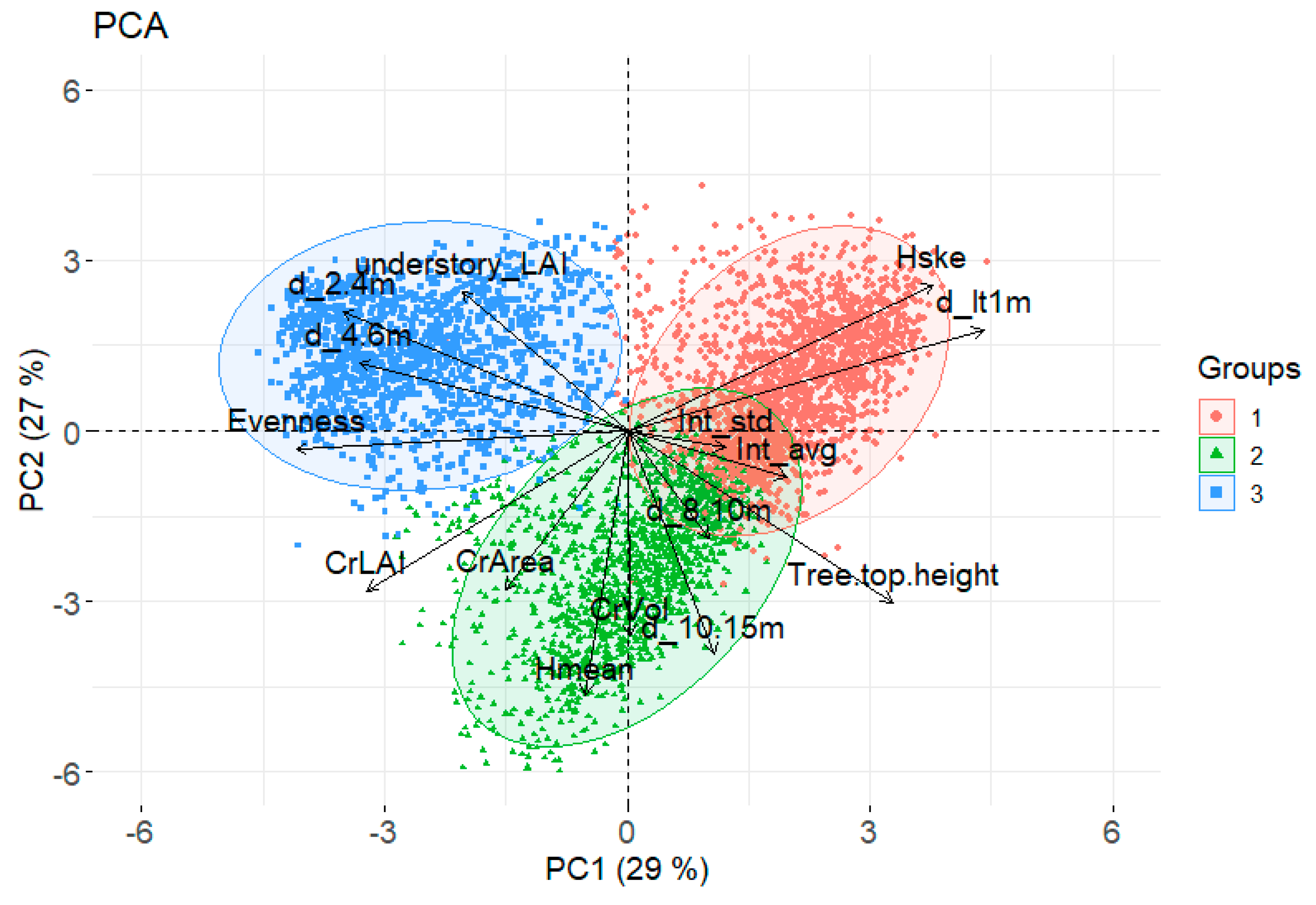
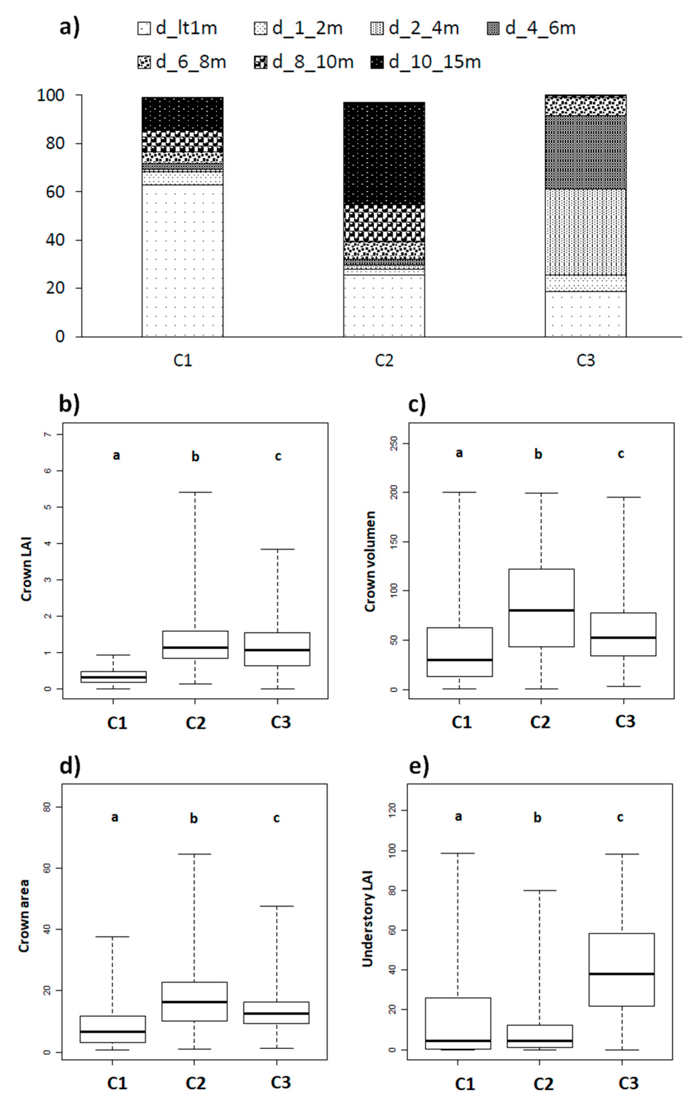
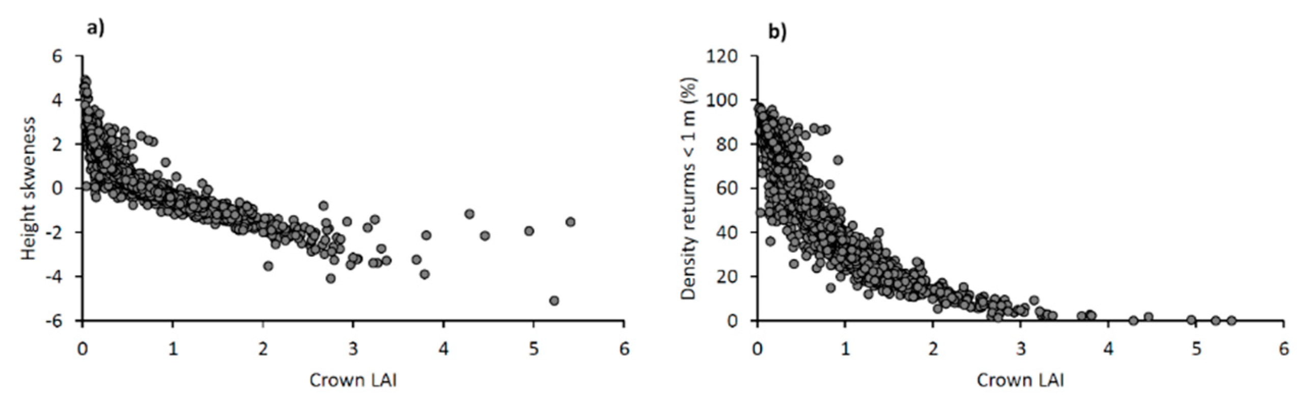
3.1. Which Structural Metrics (LiDAR-Derived) Are Most Important for Separating Individual Trees into Distinct Groups?
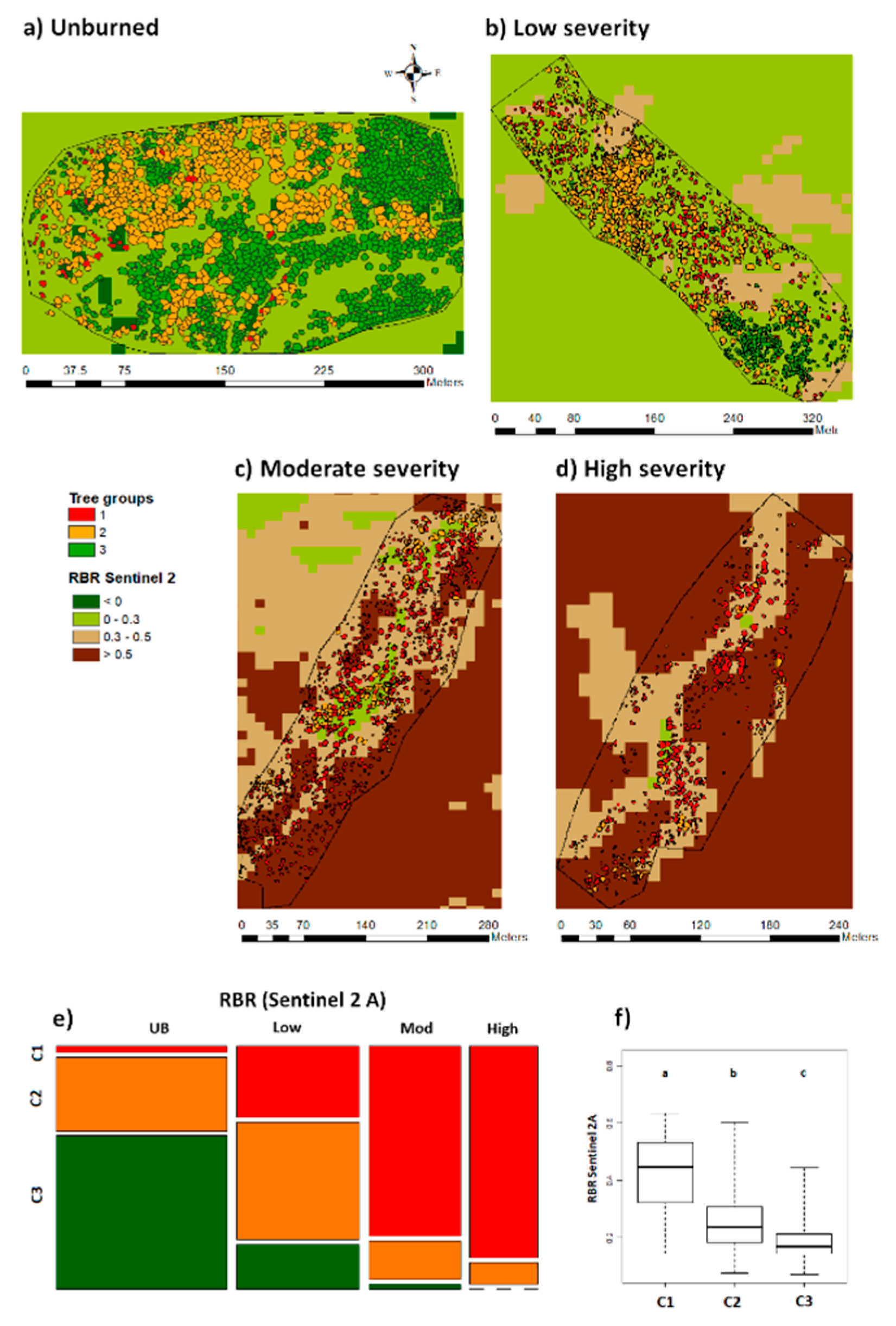
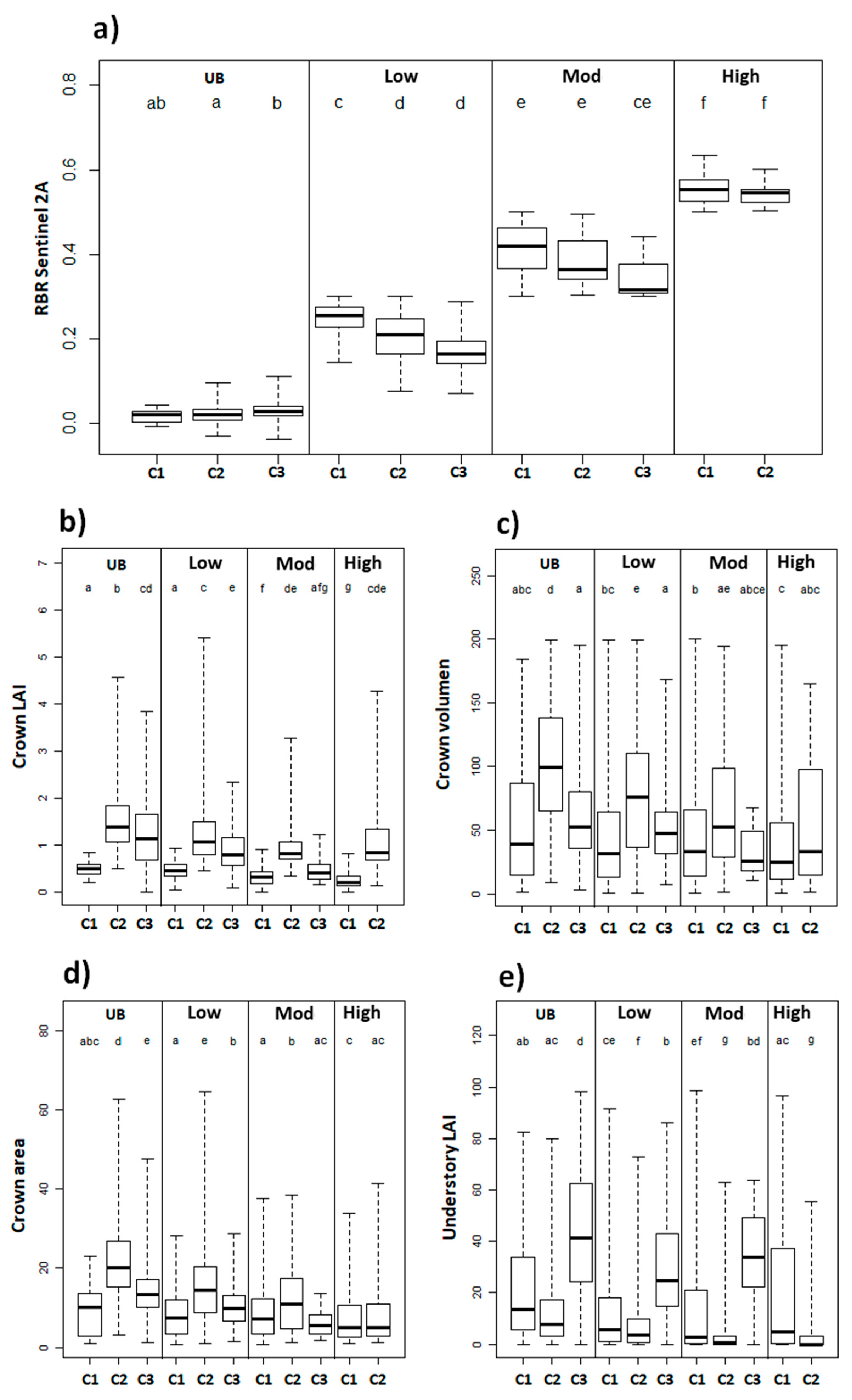
3.2. How Tree Groups Are Distributed within Fire Severity Categories
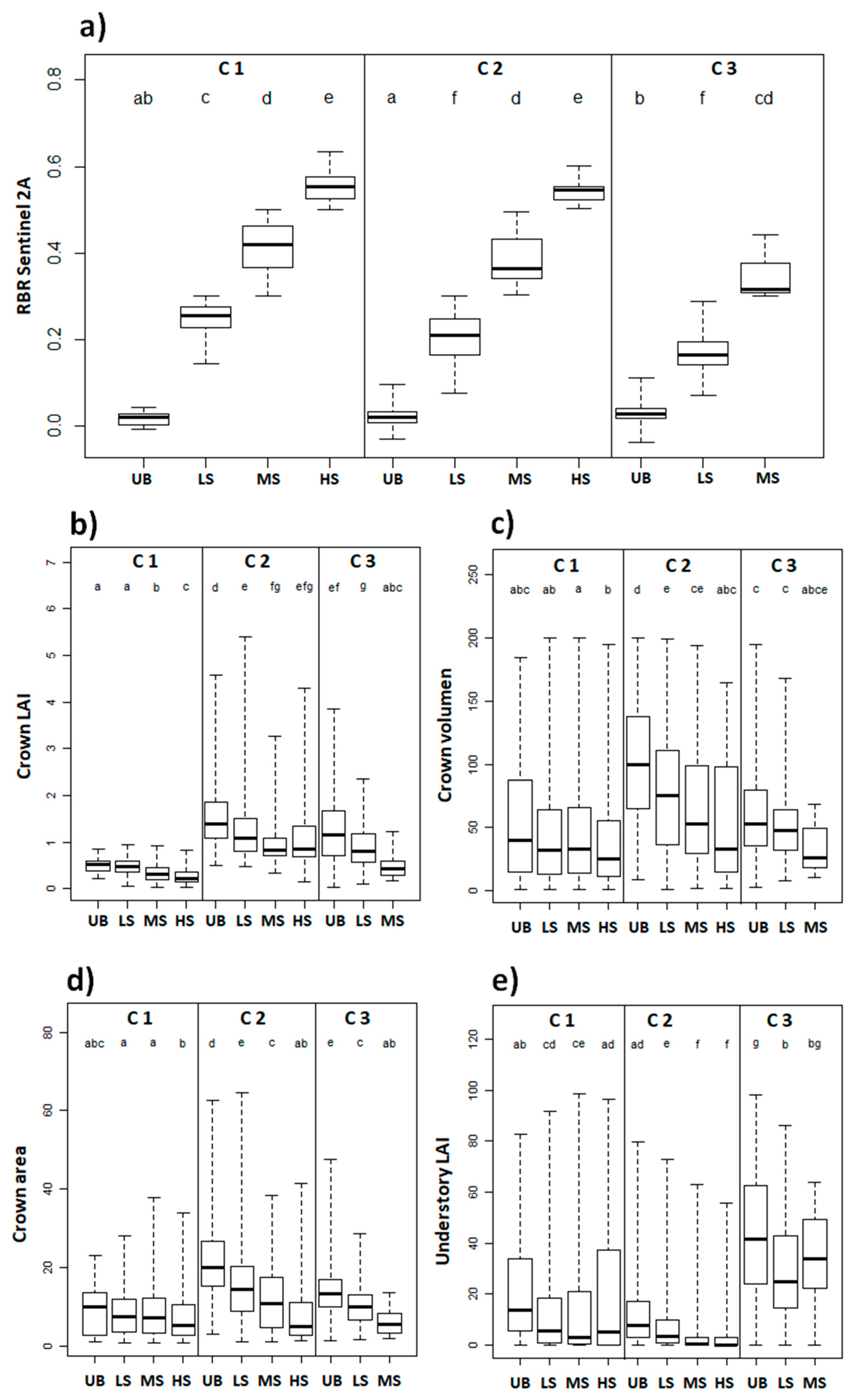
3.3. How Tree Groups Related to RBR Sentinel 2A Fire Severity Levels
4. Discussion
4.1. Which Structural Metrics (LiDAR-Derived) Are Most Important for Separating Individual Trees into Distinct Groups?
4.2. How Tree Groups Are Distributed within Fire Severity Categories
4.3. How Tree Groups Related to RBR Sentinel 2A Fire Severity Levels
4.4. Limitations and Future Work
5. Conclusions
Supplementary Materials
Author Contributions
Funding
Acknowledgments
Conflicts of Interest
References
- Moreno, J.M.; Oechel, W. A simple method for estimating fire intensity after a burn in California chaparral. Acta Oecol. 1989, 10, 57–68. [Google Scholar]
- Perez, B.; Moreno, J.M. Methods for quantifying fire severity in shrubland-fires. Plant Ecol. 1998, 139, 91–101. [Google Scholar] [CrossRef]
- Keeley, J.E. Fire intensity, fire severity and burn severity: A brief review and suggested usage. Int. J. Wildland Fire 2009, 18, 116–126. [Google Scholar] [CrossRef]
- Conard, S.G.; Sukhinin, A.I.; Stocks, B.J.; Cahoon, D.R.; Davidenko, E.P.; Ivanova, G.A. Determining Effects of Area Burned and Fire Severity on Carbon Cycling and Emissions in Siberia. Clim. Chang. 2002, 55, 197–211. [Google Scholar] [CrossRef]
- Boby, L.A.; Schuur, E.A.; Mack, M.C.; Verbyla, D.; Johnstone, J.F. Quantifying fire severity, carbon, and nitrogen emissions in Alaska’s boreal forest. Ecol. Appl. 2010, 20, 1633–1647. [Google Scholar] [CrossRef] [PubMed] [Green Version]
- Carlson, C.H.; Dobrowski, S.Z.; Safford, H.D. Variation in tree mortality and regeneration affect forest carbon recovery following fuel treatments and wildfire in the Lake Tahoe Basin, California, USA. Carbon Balance Manag. 2012, 7, 7. [Google Scholar] [CrossRef] [PubMed] [Green Version]
- Diaz-Delgado, R.; Lloret, F.; Pons, X. Influence of fire severity on plant regeneration by means of remote sensing imagery. Int. J. Remote Sens. 2003, 24, 1751–1763. [Google Scholar] [CrossRef]
- Viana-Soto, A.; Aguado, I.; Martínez, S. Assessment of post-fire vegetation recovery using fire severity and geographical data in the mediterranean region (Spain). Environments 2017, 4, 90. [Google Scholar] [CrossRef] [Green Version]
- Schoennagel, T.; Smithwick, E.A.H.; Turner, M.G. Landscape heterogeneity following large fires: Insights from Yellowstone National Park, USA. Int. J. Wildland Fire 2008, 17, 742–753. [Google Scholar] [CrossRef]
- Kim, Y.; Yang, Z.; Cohen, W.B.; Pflugmacher, D.; Lauver, C.L.; Vankat, J.L. Distinguishing between live and dead standing tree biomass on the North Rim of Grand Canyon National Park, USA using small-footprint lidar data. Remote Sens. Environ. 2009, 113, 2499–2510. [Google Scholar] [CrossRef]
- Kane, V.R.; Lutz, J.A.; Roberts, S.L.; Smith, D.F.; McGaughey, R.J.; Povak, N.A.; Brooks, M.L. Landscape-scale effects of fire severity on mixed-conifer and red fir forest structure in Yosemite National Park. For. Ecol. Manag. 2013, 287, 17–31. [Google Scholar] [CrossRef]
- Kane, V.R.; North, M.P.; Lutz, J.A.; Churchill, D.J.; Roberts, S.L.; Smith, D.F.; McGaughey, R.J.; Kane, J.T.; Brooks, M.L. Assessing fire effects on forest spatial structure using a fusion of Landsat and airborne LiDAR data in Yosemite National Park. Remote Sens. Environ. 2014, 151, 89–101. [Google Scholar] [CrossRef]
- Klauberg, C.; Hudak, A.T.; Silva, C.A.; Lewis, S.A.; Robichaud, P.R.; Jain, T.B. Characterizing fire effects on conifers at tree level from airborne laser scanning and high-resolution, multispectral satellite data. Ecol. Model. 2019, 412, 108820. [Google Scholar] [CrossRef]
- Hu, T.; Ma, Q.; Su, Y.; Battles, J.J.; Collins, B.M.; Stephens, S.L.; Kelly, M.; Guo, Q. A simple and integrated approach for fire severity assessment using bi-temporal airborne LiDAR data. Int. J. Appl. Earth Obs. Geoinf. 2019, 78, 25–38. [Google Scholar] [CrossRef]
- Hinojosa, M.B.; Albert-Belda, E.; Gómez-Muñoz, B.; Moreno, J.M. High fire frequency reduces soil fertility underneath woody plant canopies of Mediterranean ecosystems. Sci. Total Environ. 2020, 752, 141877. [Google Scholar] [CrossRef] [PubMed]
- White, J.; Ryan, K.; Key, C.; Running, S. Remote Sensing of Forest Fire Severity and Vegetation Recovery. Int. J. Wildland Fire 1996, 6, 125–136. [Google Scholar] [CrossRef] [Green Version]
- Wulder, M.; White, J.; Alvarez, F.; Han, T.; Rogan, J.; Hawkes, B. Characterizing boreal forest wildfire with multi-temporal Landsat and LIDAR data. Remote Sens. Environ. 2009, 113, 1540–1555. [Google Scholar] [CrossRef]
- Bolton, D.K.; Coops, N.C.; Wulder, M.A. Characterizing residual structure and forest recovery following high-severity fire in the western boreal of Canada using Landsat time-series and airborne lidar data. Remote Sens. Environ. 2015, 163, 48–60. [Google Scholar] [CrossRef]
- Garcia, M.; Saatchi, S.; Casas, A.; Koltunov, A.; Ustin, S.; Ramirez, C.; Garcia-Gutierrez, J.; Balzter, H. Quantifying biomass consumption and carbon release from the California Rim fire by integrating airborne LiDAR and Landsat OLI data. J. Geophys. Res. Biogeosci. 2017, 122, 340–353. [Google Scholar] [CrossRef]
- Lefsky, M.A.; Cohen, W.B.; Parker, G.G.; Harding, D.J. Lidar remote sensing for ecosystem studies. BioScience 2002, 52, 19–30. [Google Scholar] [CrossRef]
- Pflugmacher, D.; Cohen, W.B.; Kennedy, R.E.; Yang, Z. Using Landsat-derived disturbance and recovery history and lidar to map forest biomass dynamics. Remote Sens. Environ. 2014, 151, 124–137. [Google Scholar] [CrossRef]
- Wang, C.; Glenn, N.F. Estimation of fire severity using pre-and post-fire LiDAR data in sagebrush steppe rangelands. Int. J. Wildland Fire 2009, 18, 848–856. [Google Scholar] [CrossRef] [Green Version]
- Alonzo, M.; Morton, D.C.; Cook, B.D.; Andersen, H.-E.; Babcock, C.; Pattison, R. Patterns of canopy and surface layer consumption in a boreal forest fire from repeat airborne lidar. Environ. Res. Lett. 2017, 12, 065004. [Google Scholar] [CrossRef]
- Stark, S.C.; Leitold, V.; Wu, J.L.; Hunter, M.O.; de Castilho, C.V.; Costa, F.R.; McMahon, S.M.; Parker, G.G.; Shimabukuro, M.T.; Lefsky, M.A. Amazon forest carbon dynamics predicted by profiles of canopy leaf area and light environment. Ecol. Lett. 2012, 15, 1406–1414. [Google Scholar] [CrossRef] [PubMed] [Green Version]
- Almeida, D.R.A.; Nelson, B.W.; Schietti, J.; Gorgens, E.B.; Resende, A.F.; Stark, S.C.; Valbuena, R. Contrasting fire damage and fire susceptibility between seasonally flooded forest and upland forest in the Central Amazon using portable profiling LiDAR. Remote Sens. Environ. 2016, 184, 153–160. [Google Scholar] [CrossRef]
- Almeida, D.R.A.; Broadbent, E.N.; Zambrano, A.M.A.; Wilkinson, B.E.; Ferreira, M.E.; Chazdon, R.; Meli, P.; Gorgens, E.B.; Silva, C.A.; Stark, S.C.; et al. Monitoring the structure of forest restoration plantations with a drone-lidar system. Int. J. Appl. Earth Obs. Geoinf. 2019, 79, 192–198. [Google Scholar] [CrossRef]
- Almeida, D.R.A.; Almeyda Zambrano, A.M.; Broadbent, E.N.; Wendt, A.L.; Foster, P.; Wilkinson, B.E.; Salk, C.; Papa, D.D.A.; Stark, S.C.; Valbuena, R. Detecting successional changes in tropical forest structure using GatorEye drone-borne lidar. Biotropica 2020. [Google Scholar] [CrossRef]
- McCarley, T.R.; Kolden, C.A.; Vaillant, N.M.; Hudak, A.T.; Smith, A.M.; Wing, B.M.; Kellogg, B.S.; Kreitler, J. Multi-temporal LiDAR and Landsat quantification of fire-induced changes to forest structure. Remote Sens. Environ. 2017, 191, 419–432. [Google Scholar] [CrossRef] [Green Version]
- Kamoske, A.G.; Dahlin, K.M.; Stark, S.C.; Serbin, S.P. Leaf area density from airborne LiDAR: Comparing sensors and resolutions in a temperate broadleaf forest ecosystem. For. Ecol. Manag. 2019, 433, 364–375. [Google Scholar] [CrossRef]
- Falkowski, M.J.; Evans, J.S.; Martinuzzi, S.; Gessler, P.E.; Hudak, A.T. Characterizing forest succession with lidar data: An evaluation for the Inland Northwest, USA. Remote Sens. Environ. 2009, 113, 946–956. [Google Scholar] [CrossRef] [Green Version]
- Bishop, B.D.; Dietterick, B.C.; White, R.A.; Mastin, T.B. Classification of plot-level fire-caused tree mortality in a redwood forest using digital orthophotography and LiDAR. Remote Sens. 2014, 6, 1954–1972. [Google Scholar] [CrossRef] [Green Version]
- Karna, Y.K.; Penman, T.D.; Aponte, C.; Bennett, L.T. Assessing Legacy Effects of Wildfires on the Crown Structure of Fire-Tolerant Eucalypt Trees Using Airborne LiDAR Data. Remote Sens. 2019, 11, 2433. [Google Scholar] [CrossRef] [Green Version]
- Koch, B.; Heyder, U.; Weinacker, H. Detection of Individual Tree Crowns in Airborne Lidar Data. Photogramm. Eng. Remote Sens. 2006, 72, 357–363. [Google Scholar] [CrossRef] [Green Version]
- Hu, B.; Li, J.; Jing, L.; Judah, A. Improving the efficiency and accuracy of individual tree crown delineation from high-density LiDAR data. Int. J. Appl. Earth Obs. Geoinf. 2014, 26, 145–155. [Google Scholar] [CrossRef]
- Wu, B.; Yu, B.; Wu, Q.; Huang, Y.; Chen, Z.; Wu, J. Individual tree crown delineation using localized contour tree method and airborne LiDAR data in coniferous forests. Int. J. Appl. Earth Obs. Geoinf. 2016, 52, 82–94. [Google Scholar] [CrossRef]
- Jeronimo, S.M.; Kane, V.R.; Churchill, D.J.; McGaughey, R.J.; Franklin, J.F. Applying LiDAR individual tree detection to management of structurally diverse forest landscapes. J. For. 2018, 116, 336–346. [Google Scholar] [CrossRef] [Green Version]
- Wiggins, H.L.; Nelson, C.R.; Larson, A.J.; Safford, H.D. Using LiDAR to develop high-resolution reference models of forest structure and spatial pattern. For. Ecol. Manag. 2019, 434, 318–330. [Google Scholar] [CrossRef]
- González-Ferreiro, E.; Arellano-Pérez, S.; Castedo-Dorado, F.; Hevia, A.; Vega, J.A.; Vega-Nieva, D.; Álvarez-González, J.G.; Ruiz-González, A.D. Modelling the vertical distribution of canopy fuel load using national forest inventory and low-density airbone laser scanning data. PLoS ONE 2017, 12, e0176114. [Google Scholar] [CrossRef]
- Morsdorf, F.; Meier, E.; Kötz, B.; Itten, K.I.; Dobbertin, M.; Allgöwer, B. LIDAR-based geometric reconstruction of boreal type forest stands at single tree level for forest and wildland fire management. Remote Sens. Environ. 2004, 92, 353–362. [Google Scholar] [CrossRef]
- Maltamo, M.; Mustonen, K.; Hyyppä, J.; Pitkänen, J.; Yu, X. The accuracy of estimating individual tree variables with airborne laser scanning in a boreal nature reserve. Can. J. For. Res. 2004, 34, 1791–1801. [Google Scholar]
- Omasa, K.; Akiyama, Y.; Ishigami, Y.; Yoshimi, K. 3-D remote sensing of woody canopy heights using a scanning helicopter-borne lidar system with high spatial resolution. J. Remote Sens. Soc. Jpn. 2000, 20, 394–406. [Google Scholar]
- Omasa, K.; Qiu, G.Y.; Watanuki, K.; Yoshimi, K.; Akiyama, Y. Accurate estimation of forest carbon stocks by 3-D remote sensing of individual trees. Environ. Sci. Technol. 2003, 37, 1198–1201. [Google Scholar] [CrossRef] [PubMed]
- Omasa, K.; Hosoi, F.; Konishi, A. 3D lidar imaging for detecting and understanding plant responses and canopy structure. J. Exp. Bot. 2007, 58, 881–898. [Google Scholar] [CrossRef] [Green Version]
- Hosoi, F.; Nakai, Y.; Omasa, K. Estimation and error analysis of woody canopy leaf area density profiles using 3-D airborne and ground-based scanning lidar remote-sensing techniques. IEEE Trans. Geosci. Remote Sens. 2010, 48, 2215–2223. [Google Scholar] [CrossRef]
- Stark, S.C.; Enquist, B.J.; Saleska, S.R.; Leitold, V.; Schietti, J.; Longo, M.; Alves, L.F.; Camargo, P.B.; Oliveira, R.C. Linking canopy leaf area and light environments with tree size distributions to explain Amazon forest demography. Ecol. Lett. 2015, 18, 636–645. [Google Scholar] [CrossRef]
- Hosoi, F.; Omasa, K. Voxel-based 3-D modeling of individual trees for estimating leaf area density using high-resolution portable scanning lidar. IEEE Trans. Geosci. Remote Sens. 2006, 44, 3610–3618. [Google Scholar] [CrossRef]
- Almeida, D.R.A.d.; Stark, S.C.; Shao, G.; Schietti, J.; Nelson, B.W.; Silva, C.A.; Gorgens, E.B.; Valbuena, R.; Papa, D.A.; Brancalion, P.H.S. Optimizing the remote detection of tropical rainforest structure with airborne lidar: Leaf area profile sensitivity to pulse density and spatial sampling. Remote Sens. 2019, 11, 92. [Google Scholar] [CrossRef] [Green Version]
- Popescu, S.C.; Zhao, K. A voxel-based lidar method for estimating crown base height for deciduous and pine trees. Remote Sens. Environ. 2008, 112, 767–781. [Google Scholar] [CrossRef]
- Luo, L.; Zhai, Q.; Su, Y.; Ma, Q.; Kelly, M.; Guo, Q. Simple method for direct crown base height estimation of individual conifer trees using airborne LiDAR data. Opt. Express 2018, 26, A562–A578. [Google Scholar] [CrossRef]
- Næsset, E. Practical large-scale forest stand inventory using a small-footprint airborne scanning laser. Scand. J. For. Res. 2004, 19, 164–179. [Google Scholar] [CrossRef]
- Angelo, J.J.; Duncan, B.W.; Weishampel, J.F. Using lidar-derived vegetation profiles to predict time since fire in an oak scrub landscape in East-Central Florida. Remote Sens. 2010, 2, 514–525. [Google Scholar] [CrossRef] [Green Version]
- Goetz, S.J.; Sun, M.; Baccini, A.; Beck, P.S. Synergistic use of spaceborne lidar and optical imagery for assessing forest disturbance: An Alaska case study. J. Geophys. Res. Biogeosci. 2010, 115. [Google Scholar] [CrossRef] [Green Version]
- Viedma, O.; Chico, F.; Fernández, J.; Madrigal, C.; Safford, H.; Moreno, J. Disentangling the role of prefire vegetation vs. burning conditions on fire severity in a large forest fire in SE Spain. Remote Sens. Environ. 2020, 247, 111891. [Google Scholar] [CrossRef]
- LidarPod. Available online: https://grafinta.com/wp-content/uploads/2017/05/TerraSystem-LidarPod-LidarViewer_GSA.pdf (accessed on 1 February 2020).
- Kinematica. Available online: https://hq.advancednavigation.com.au/kinematica/login.jsp (accessed on 15 March 2020).
- LasTools. Available online: http://lastools.org/ (accessed on 20 March 2020).
- National, I.G. Available online: ftp://ftp.geodesia.ign.es/geoide/ (accessed on 21 March 2019).
- Roussel, J.-R.; Auty, D.; De Boissieu, F.; Meador, A. lidR: Airborne LiDAR data manipulation and visualization for forestry applications. R Package Version 2018, 1, 1. [Google Scholar]
- Team, R. R: A Language and Environment for Statistical Computing; R Foundation for Statistical Computing: Vienna, Austria, 2011; Available online: https://www.R-project.org (accessed on 1 August 2020).
- Khosravipour, A.; Skidmore, A.K.; Isenburg, M. Generating spike-free digital surface models using LiDAR raw point clouds: A new approach for forestry applications. Int. J. Appl. Earth Obs. Geoinf. 2016, 52, 104–114. [Google Scholar] [CrossRef]
- Silva, C.A.; Hudak, A.T.; Vierling, L.A.; Loudermilk, E.L.; O’Brien, J.J.; Hiers, J.K.; Jack, S.B.; Gonzalez-Benecke, C.; Lee, H.; Falkowski, M.J. Imputation of individual longleaf pine (Pinus palustris Mill.) tree attributes from field and LiDAR data. Can. J. Remote Sens. 2016, 42, 554–573. [Google Scholar] [CrossRef]
- Hijmans, R.; Van Etten, J. Raster: Geographic Data Analysis and Modeling; R package version 2.5-8; 2016. Available online: https://cran.microsoft.com/snapshot/2016-08-05/web/packages/raster/index.html (accessed on 20 October 2020).
- Kindt, R.; Coe, R. Tree Diversity Analysis: A Manual and Software for Common Statistical Methods for Ecological and Biodiversity Studies; World Agroforestry Centre: Nairobi, Kenya, 2005. [Google Scholar]
- Casas, Á.; García, M.; Siegel, R.B.; Koltunov, A.; Ramírez, C.; Ustin, S. Burned forest characterization at single-tree level with airborne laser scanning for assessing wildlife habitat. Remote Sens. Environ. 2016, 175, 231–241. [Google Scholar] [CrossRef] [Green Version]
- Zeileis, A.; Kleiber, C.; Krämer, W.; Hornik, K. Testing and dating of structural changes in practice. Comput. Stat. Data Anal. 2003, 44, 109–123. [Google Scholar] [CrossRef] [Green Version]
- Copernicus. Available online: https://scihub.copernicus.eu/ (accessed on 1 February 2019).
- SNAP. Available online: https://step.esa.int/main/snap-6-0-released/ (accessed on 15 February 2019).
- Parks, S.A.; Dillon, G.K.; Miller, C. A new metric for quantifying burn severity: The relativized burn ratio. Remote Sens. 2014, 6, 1827–1844. [Google Scholar] [CrossRef] [Green Version]
- Breiman, L. Random forests. Mach. Learn. 2001, 45, 5–32. [Google Scholar] [CrossRef] [Green Version]
- Lê, S.; Josse, J.; Husson, F. FactoMineR: An R package for multivariate analysis. J. Stat. Softw. 2008, 25, 1–18. [Google Scholar] [CrossRef] [Green Version]
- Moritz, M.A.; Batllori, E.; Bradstock, R.A.; Gill, A.M.; Handmer, J.; Hessburg, P.F.; Leonard, J.; McCaffrey, S.; Odion, D.C.; Schoennagel, T. Learning to coexist with wildfire. Nature 2014, 515, 58–66. [Google Scholar] [CrossRef] [PubMed]
- Asner, G.P.; Kellner, J.R.; Kennedy-Bowdoin, T.; Knapp, D.E.; Anderson, C.; Martin, R.E. Forest Canopy Gap Distributions in the Southern Peruvian Amazon. PLoS ONE 2013, 8, e60875. [Google Scholar] [CrossRef] [Green Version]


| Type of Metric | LiDAR Metrics at Tree Level | Description | Source |
|---|---|---|---|
| Crown metrics | Crown metrics | Canopy Height Model (CHM) | |
| Treetop height (m) | Height of the treetop (m) | ||
| Crown area | Area of segmented crowns (Silva’s method) (m2) | ||
| Relative Understory LAI | LAI (0–2.5 m) (%) | Voxelized vertical canopy profiles (VCPs) | |
| Crown LAI | Total LAI—Understory LAI | ||
| Crown volume | Crown length * Crown area (m3) | ||
| Cloud metrics | All points and height strata (<4 m and >4 m) | Min, max, average | Raw points |
| standard deviation, kurtosis and skewness | |||
| Percentiles * | |||
| Vegetation cover (%) | Height ranges ** | ||
| Diversity metrics | Shannon and Richness | From 0 to 20 m at 0.5 m intervals | Density of height bins |
| Evenness |
Publisher’s Note: MDPI stays neutral with regard to jurisdictional claims in published maps and institutional affiliations. |
© 2020 by the authors. Licensee MDPI, Basel, Switzerland. This article is an open access article distributed under the terms and conditions of the Creative Commons Attribution (CC BY) license (http://creativecommons.org/licenses/by/4.0/).
Share and Cite
Viedma, O.; Almeida, D.R.A.; Moreno, J.M. Postfire Tree Structure from High-Resolution LiDAR and RBR Sentinel 2A Fire Severity Metrics in a Pinus halepensis-Dominated Burned Stand. Remote Sens. 2020, 12, 3554. https://doi.org/10.3390/rs12213554
Viedma O, Almeida DRA, Moreno JM. Postfire Tree Structure from High-Resolution LiDAR and RBR Sentinel 2A Fire Severity Metrics in a Pinus halepensis-Dominated Burned Stand. Remote Sensing. 2020; 12(21):3554. https://doi.org/10.3390/rs12213554
Chicago/Turabian StyleViedma, Olga, Danilo R. A. Almeida, and Jose Manuel Moreno. 2020. "Postfire Tree Structure from High-Resolution LiDAR and RBR Sentinel 2A Fire Severity Metrics in a Pinus halepensis-Dominated Burned Stand" Remote Sensing 12, no. 21: 3554. https://doi.org/10.3390/rs12213554