Moving Target Detection in Multi-Static GNSS-Based Passive Radar Based on Multi-Bernoulli Filter

Abstract

Over the past few years, the global navigation satellite system (GNSS)-based passive radar (GBPR) has attracted more and more attention and has developed very quickly. However, the low power level of GNSS signal limits its application. To enhance the ability of moving target detection, a multi-static GBPR (MsGBPR) system is considered in this paper, and a modified iterated-corrector multi-Bernoulli (ICMB) filter is also proposed. The likelihood ratio model of the MsGBPR with range-Doppler map is first presented. Then, a signal-to-noise ratio (SNR) online estimation method is proposed, which can estimate the fluctuating and unknown map SNR effectively. After that, a modified ICMB filter and its sequential Monte Carlo (SMC) implementation are proposed, which can update all measurements from multi-transmitters in the optimum order (ascending order). Moreover, based on the proposed method, a moving target detecting framework using MsGBPR data is also presented. Finally, performance of the proposed method is demonstrated by numerical simulations and preliminary experimental results, and it is shown that the position and velocity of the moving target can be estimated accurately.

1. Introduction

Compared with other opportunistic illuminators, the global navigation satellite system (GNSS) is a good choice for passive radar given its permanent global coverage, plentiful satellite resources and ease for synchronization [1,2,3,4]. Therefore, the GNSS-based passive radar (GBPR) is an innovative, all-weather, and all-time microwave tool for remote sensing and target detection applications, and it has developed very quickly in recent years [5,6,7,8,9,10,11,12,13,14,15].

To overcome the low power level for target detection in a GBPR system, advanced signal processing methods, such as SAR imaging and two-dimensional (2-D) coherent integration [10,11,12,13], are needed to achieve the 2-D coherent integration gain [14,15]. Normally, the GBPR system is based on the bi-static model, where a single GNSS satellite is used as the transmitter. However, GNSS constellations (GPS, BeiDou, GLONASS, and Galileo) possess over 100 satellites, and multiple azimuth and elevation angle observations are available for target illumination in any given area [1,2]; on the other hand, the pseudo random noise (PRN) codes used in GNSS have excellent auto-correlation and cross-correlation properties [3]. As a result, it is feasible to employ multiple transmitters in a GBPR system at the same time, and the echo signal from each transmitter can be easily separated by the corresponding PRN code.

Our research in this work is focused on moving target detection using a multi-static GBPR (MsGBPR) system, so that information from different observation perspectives can be fully utilized for enhanced detection ability and more effective detection performance. For such a multi-sensor detection problem, centralized, distributed or decentralized architectures are commonly used, and the centralized one is the optimal architecture in terms of detection performance [16]. A comprehensive overview of multi-sensor-based detection techniques can be found in [16,17,18] and references therein. The Random Finite Set (RFS) and Finite Set Statistics (FISST) frameworks proposed by Mahler [17,18] have gained much attention and several popular filters such as the probability hypothesis density (PHD) filter [19], the cardinalized PHD (CPHD) filter [20], the multi-Bernoulli (MB) filter [21], the Poisson MB mixture (PMBM) filter [22], and the generalized labeled MB (GLMB) filter [23,24], have been developed based on the FISST framework. These filters also belong to the track-before-detect (TBD) technique [25], which is suitable for low signal-to-noise ratio (SNR) applications, as it minimizes information loss by sidestepping the detection implementation [25,26,27,28,29]. Thus, these filters are good candidates for target detection in MsGBPR with its low power level. The PHD filter and MB filter with subsequent improvements were proposed to cater for multi-sensor applications [30,31,32,33,34,35,36,37,38,39]. Compared with the class of PHD filters, the MB-based is more efficient and accurate if each target’s existence probability is required [21,39], and the performance of MB-based filters has been well demonstrated in many practical applications, such as computer vision [40], acoustic sensor tracking [41], and sensor control [42,43].

The update strategy is another crucial problem in multi-sensor systems [16,18,22,37,44]. In MsGBPR, a single receiver records all target reflected GNSS signals from multiple transmitters, and this can be considered as some kind of centralized architecture. Two well-known strategies for updating in a centralized fusion center are sequential updating and super-measurements updating [18,44]. In super-measurement updating, all measurements are first associated to generate a super-measurement, such as the joint likelihood function method; then, the super-measurement will be treated as the measurement by a single sensor [16]. In this way, the multi-sensor detection problem is converted into a single sensor detection problem. However, as the joint likelihood function is the product of each sensor’s likelihood function, the performance of super-measurement updating is highly dependent on the quality of measurements. In sequential updating, the posterior target state estimated by the measurement from the i-th sensor will be used as the prior information when the measurement from the i + 1-th sensor is being processed [16], such as the iterated-corrected PHD (ICPHD) [18,45] and iterated-corrector MB (ICMB) filters [37]. Generally, the sequential updating strategy will yield the best solution, but the estimated result depends on whether the higher quality measurement is used first or last in the sequential updating [18,44]. In MsGBPR, the target will be illuminated from multiple azimuth and elevation angles, which will lead to fluctuating SNR levels for different measurements. As the moving target is non-cooperative, the SNR of each measurement is normally unknown. Therefore, it is difficult to decide the update order if the sequential updating strategy is employed.

In this paper, motivated by previous works on 2-D coherent processing, the multi-sensor MB filter is employed in the MsGBPR system for moving target detection. Firstly, the likelihood ratio function in MsGBPR is modeled based on the range-Doppler map. Then, the product MB (PMB) filter and ICMB filter are introduced for target detection in MsGBPR. After that, based on the principle of maximum likelihood estimation, a modified ICMB filter with an online SNR estimation and its sequential Monte Carlo (SMC) implementation are proposed, which can update all measurements in the optimum order and get the best output from the ICMB filter for detection. Finally, the whole moving target detection framework in MsGBPR is presented, including echo separation, 2-D coherent integration, target state estimation by the proposed filter, and target track generation.

This paper is organized as follows. Geometry of the MsGBPR system and its 2-D coherent integration result in range-Doppler domain are presented in Section 2. Then, in Section 3, the modified ICMB filter using MsGBPR data is derived in detail, with its sequential Monte Carlo (SMC) implementation. Furthermore, the moving target detection framework for MsGBPR system is also introduced. In Section 4, numerical simulations are carried out to demonstrate the validity and feasibility of the proposed modified ICMB filter. Discussion about the performance and the computational efficiency improvement by the modified ICMB filter are given in Section 5. In Section 6, preliminary experimental results using GPS signals are also presented to demonstrate the effectiveness of the proposed modified ICMB filter. Section 7 concludes the paper with possible future research directions.

2. MsGBPR System and Its Signal Model

First of all, the general geometric configuration of an MsGBPR system is described and the echo model for a moving target is derived based on the GNSS signal and MsGBPR acquisition geometry. Then, the map results of a moving target in the MsGBPR system are presented based on 2-D coherent integration processing.

2.1. Geometry of MsGBPR and Moving Target Echo Model

Figure 1 shows the general geometric configuration of an MsGBPR system for moving target detection. For MsGBPR, multi-angle observations from over 20 satellites (GPS, BeiDou, GLONASS, and Galileo) in any given area are attainable, and to simplify, only one receiver is employed, which is located at the origin of the Cartesian coordinate system, as shown in Figure 1, where the X-axis points to the North direction and the Y-axis points to the West direction. The moving target P is located at P_tar(X_A, Y_A, Z_A) with a constant velocity V_tar(V_x, V_y, 0). Furthermore, multiple global navigation satellites are used as transmitters denoted by Tⁱ, as shown in Figure 1, where i = 1, 2, 3, … For each transmitter Tⁱ, its position vector and velocity vector are represented by $P_{Tran}^i$ and $V_{Tran}^i$, respectively, and both can be obtained precisely using the ephemerides of GNSS satellites.

The radar system’s range history is a crucial factor for signal processing and target detection. Considering the link of the i-th transmitter, target and receiver, the range history R_i(η) can be modeled as [11,12]

$$R_i\left(\eta \right)={\Vert P_{Tran,i}^{}-P_{tar}^{}\Vert }_2+{\Vert P_{tar}^{}\Vert }_2=R_{ref,i}^{}+\lambda f_{d,i}^{}\eta +\frac{\lambda }{2}{f}_{r,i}^{}{\eta }^2$$

(1)

where λ is the signal wavelength, η is the illumination time, R_ref,i, f_d,i and f_r,i denote the reference range, Doppler centroid, and Doppler modulated rate with the geometry of the i-th transmitter at the center illumination time, and their detailed calculation method can be found in [14].

Then, according to [14], after quadrature demodulation and synchronization, the 2-D form of the echo signal can be written as

$$S\left(t,\tau \right)={\displaystyle \sum _{i=1}^I{\zeta }_i{A}_T{Q}_i\left[\tau -\frac{R_i\left(t\right)}{c}\right]\exp \left\{-j\frac{2\pi R_i\left(t\right)}{\lambda }\right\}}·\exp \left\{-j2\pi f_{d,i}^{}\tau \right\}$$

(2)

where t is the slow time, τ is the fast time, A_T is the signal amplitude, Q_i(·) is the modulation code of the i-th transmitter, c is the speed of light, and ζ_i is the target radar cross-section (RCS) associated with the geometry of the i-th transmitter. It should be noted that σ_i is changing with the observation angle, so it may be different for each transmitter geometry. As in (2), the received echo signal of MsGBPR is actually the summation of all reflected signals from visible transmitters (satellites), and it is easy to separate them by each satellite’s PRN code, as it has excellent auto-correlation and cross-correlation properties. Unlike the “stop-and-go” approximation in traditional radar [46], the moving of transmitter during the fast time in GBPR should also be considered. Hence, as shown in (2), the Doppler effect during the fast time needs to be taken into consideration, and it should be carefully dealt with during the 2-D coherent integration processing [14].

2.2. 2-D Coherent Integration Map Results of Moving Target

As the power level of MsGBPR echo signals is very low, long time 2-D coherent integration processing is necessary to achieve sufficiently high SNR for effective target detection. Based on the principle of Radon Fourier Transform (RFT), a modified RFT method is proposed in [14], with range-walk removal, RFT, range compression and phase error compensation. A fast implementation with Chirp-Z transform is also presented in [14]. Based on the modified RFT, the diagrammatic sketch of 2-D coherent integration processing and imaging results by MsGBPR are presented in Figure 2. As shown, all visible reflected echo signals are recorded, and multiple range compression results can be obtained using the PRN code of each satellite. Then, moving targets will be focused in the range-Doppler domain by azimuth coherent processing. The range history and Doppler frequency of each geometry configuration (different transmitter used) are totally different. Therefore, as shown in Figure 2, the same target can be located in different range and Doppler cells, which will increase the difficulty of multi-target detection.

According to [14], the moving target in GNSS-based radar can be focused in range-Doppler domain, which is

$$S_o^i\left(f_v,R\right)=A_T{\zeta }_i{Q}_c{\displaystyle \sum _{m=-N_A/2}^{N_A/2-1}{D}_i\left[R-R_{ref,i}^{}+\lambda \left(f_v-f_{dv,i}^{}\right)m{T}_p\right]}·\exp \left\{j2\pi \left(f_v-f_{dv,i}^{}\right)m{T}_p\right\}$$

(3)

where Q_C is the gain of range compression, D(·) is the normalized envelope of the auto-correlation result of the i-th transmitted signal, D(0) = 1, $f_{d,v}^i$ is the Doppler frequency caused by target motion, T_p is the signal period, and N_A denotes the azimuth sample number. It should be noted that the reference range R_ref,i, and target Doppler frequency f_dv,i will change as a different geometry with the i-th transmitter is used.

Clearly, the maximum value will occur at the position of target motion parameter (R_ref,i, f_dv,i), and as in (3), $S_o^i\left(f_{dv,i}^{},R_{ref,i}^{}\right)=A_T{\zeta }_i{Q}_C{N}_A$, which equals the coherent integration gain. With the method in [14], the 2-D coherent integration gain of several even tens of seconds of echo data can still be achieved.

3. Moving Target Detection Based on Modified Multi-Bernoulli Filter

In this paper, the MsGBPR system consists of one receiver and multiple transmitters, and the echo signal from each transmitter can be separated by the PRN code. Therefore, the centralized architecture is easy to implement in MsGBPR, and the receiver is the central fusion center. As multiple transmitters are used in MsGBPR, as many as I (number of observable satellites) maps of moving targets can be acquired at the same time, which can be used to improve the target detection performance of the system.

To fully utilize all measurements (map results), multi-sensor target tracking solutions are needed. The multi-Bernoulli filter is a famous tool for multi-sensor systems, which is based on the finite set statistics framework, and it has been widely researched in applications like maneuvering targets, field robotics, and computer vision. Furthermore, the multi-Bernoulli filter is a kind of TBD method, it sidesteps the detection by leveraging spatiotemporal information directly from the map results, and is capable of detecting a moving target with SNR as low as 7 dB [29]. Therefore, less coherent integration time is needed or its detection range will increase significantly if the multi-Bernoulli filter is employed.

In this section, both the PMB filter and the ICMB filter for MsGBPR target detection are introduced. To update the multiple map results in the optimal order, a modified ICMB filter with online SNR estimation is proposed. Based on this, a framework for moving target detection in MsGBPR is also presented.

3.1. Multi-Bernoulli RFS and Multi-Bernoulli Filter

A multi-Bernoulli RFS X is a union of a certain number of independent Bernoulli RFSs, which can be expressed as $X={\displaystyle {\cup }_{q=1}^M{X}^t}$. Its existence probability is r^q ∈ (0, 1), and its probability density is p^q(·). The probability generation functional of a multi-Bernoulli RFS is [21,37]

$$G\left[h\right]={\displaystyle \prod _{i=1}^M\left(1-r^q+r^q\langle p^q,h\rangle \right)}$$

(4)

where $\langle p^q,h\rangle ={\displaystyle \int p^q\left(x\right)h}\left(x\right)dx$. Therefore, a multi-Bernoulli RFS can be represented by the parameter set $\pi ={\left\{\left(r^q,p^q\right)\right\}}_{q=1}^M$. The mean cardinality of a multi-Bernoulli RFS is ${\displaystyle {\sum }_{q=1}^M{r}^q}$, and the probability density is [21,36]

$$\pi \left(X\right)=\{\begin{array}{cc}{\displaystyle \prod _{t=1}^M\left(1-r^q\right),}& n=0\\ {\displaystyle \prod _{q=1}^M\left(1-r^q\right)}{\displaystyle \sum _{q\le q_1\ne \dots \ne q_n\le M}{\displaystyle \prod _{j=1}^n\frac{r^{q_j}{p}^{q_j}\left(x_j\right)}{1-r^{q_j}},}}& n\le m\\ 0,& n>m\end{array}$$

(5)

Based on the Bayesian recursive framework, the process of a traditional multi-Bernoulli filter can be described as follows.

Prediction: The posterior target density is a multi-Bernoulli parameter set ${\pi }_{k-1}={\left\{\left(r_{k-1}^q,p_{k-1}^q\right)\right\}}_{q=1}^{N_{k-1}}$ at sample time k − 1. Then, the predicted target density is also a multi-Bernoulli RFS, which is [27]

$${\pi }_{k|k-1}={\left\{\left(r_{P,k|k-1}^q,p_{P,k|k-1}^q\right)\right\}}_{q=1}^{N_{k|k-1}}\cup {\left\{\left(r_{\mathrm{\Gamma },k}^q,p_{\mathrm{\Gamma },k}^q\right)\right\}}_{q=1}^{N_{\mathrm{\Gamma },k}}$$

(6)

where $r_{P,k|k-1}^q=r_{k-1}^q\langle p_{k-1}^q,p_{s,k}\rangle$, $p_{P,k|k-1}^q\left(x\right)=\frac{\langle f_{k|k-1}^{}\left(x|·\right),p_{k-1}^q{p}_{s,k}\rangle }{\langle p_{k-1}^q,p_{s,k}\rangle }$, $f_{k|k-1}^{}\left(x|·\right)$ is the single target transition density at time k, p_s,k is the target existence probability at time k, and the second part in (6) is the multi-Bernoulli RFS of newborn targets at time k.

Update: The predicted target density is a multi-Bernoulli parameter set ${\pi }_{k|k-1}={\left\{\left(r_{k|k-1}^q,p_{k|k-1}^q\right)\right\}}_{q=1}^{N_{k|k-1}}$ at time k. Then, the posterior target density can be approximated by a multi-Bernoulli RFS [27]

$${\pi }_k={\left\{\left(r_k^q,p_k^q\right)\right\}}_{q=1}^{N_{k|k-1}}$$

(7)

$$\begin{gathered} r_k^q={\frac{r_{k|k-1}^q\langle p_{k|k-1}^q,L\left(z_k|x_k,e_k\right)\rangle }{1-r_{k|k-1}^q+r_{k|k-1}^q\langle p_{k|k-1}^q,L\left(z_k|x_k,e_k\right)\rangle }}_{x_k\in X_k,z_k\in Z_k}, \\ {p}_k^q={\frac{p_{k|k-1}^{q}L\left(z_k|x_k,e_k\right)}{\langle p_{k|k-1}^q,L\left(z_k|x_k,e_k\right)\rangle }}_{x_k\in X_k,z_k\in Z_k} \end{gathered}$$

(8)

where X_k is target state RFS, Z_k is the measurement RFS, and L(·) is the likelihood ratio function.

The relationship between Bayesian recursive and multi-Bernoulli filter and their propagation track table are shown in Figure 3. As shown, the target posterior density and target Bayes recursion are performed in a Bayesian filter, and based on RFS, a multi-Bernoulli parameter set is used in prediction and update.

3.2. Multi-Beroulli Filtering for Target Detection in MsGBPR

Based on the introduction in Section 3.1, the multi-Bernoulli filter application for target detection in MsGBPR is carried out. Firstly, based on the range-Doppler imaging results, the target model, measurement model and likelihood ratio function are provided. Then, the PMB filter and ICMB filter are presented based on the likelihood ratio function.

3.2.1. Target Model, Measurement Model and Likelihood Ratio Function in MsGBPR

In this paper, targets are assumed to move at a constant speed in the plane, and the target state vector is given by x = [A, x, y, v_x, v_y]^T, where A denotes the amplitude, x and y denote the target positions, and v_x and v_y are its velocities. Therefore, the traditional target kinematic model can be used for the description of target state transition.

Suppose there are N(k) targets at time k, and their target states are x_k,1, …, x_k,N(k). Then, the target states RFS is $X_k=\left\{x_{k,1},\dots ,x_{k,N(k)}\right\}\in \mathcal{F}(\mathcal{X})$. Each target x_k,qbelongs toX_k at time k, either continues to exist at time k + 1 with probability p_s,k,q(x_k,q) and new state x_k+1,q, or dies with probability 1 − p_s,k,q(x_k,q). Consequently, for a given target x_k,q at time k, its behavior at time k + 1 can be modeled by the Bernoulli RFS S_k+1|k(x_k,q). If this target still exists, S_k+1|k(x_k,q) is {x_k,q}, and if this target dies, S_k+1|k(x_k,q) becomes empty set.In addition, new targets could appear at time k + 1. Therefore, target state X_k+1 consists of two parts: existing targets since the last time and new emerging targets, and the RFS X_k+1 at time k + 1 is given by the union [27]

$$X_{k+1}=\left[{\displaystyle \underset{x_k\in X_k}{\overset{}{\cup }}{S}_{k+1|k}\left(x_k\right)}\right]{\displaystyle \cup {\Gamma }_{k+1}}$$

(9)

where ${\Gamma }_{k+1}$ is the multi-Bernoulli RFS of new born targets.

For measurements or observations in a MsGBPR system, the moving target is focused in the range-Doppler plane, and multiple imaging results can be obtained at each time. Normally, each moving target has a different Doppler frequency and range in MsGBPR, which means there is only one moving target in a pixel unit of the range-Doppler imaging result with no overlapping with each other. Then, considering whether the target exists or not at time k, the map measurement of MsGBPR with the i-th transmitter is given by

$$Z_{k,i}=\{\begin{array}{ll}{\displaystyle \sum _{q=1}^{N\left(k\right)}{g}_{k,i}^{}\left(x_k\right)}+v_{k,i}^{},& e_k=e\\ v_{k,i}^{},& e_k=\overline{e}\end{array}$$

(10)

where Z_k,i is the i-th measurement at time k, v_k,i is the complex Gaussian noise, with mean value 0 and variance ${\sigma }_i^2$, e_k is a target model variable indicating whether the target exists at time k or not, and g_k,i(x_k) is the target response function, as presented in (3). Moreover, target motion parameters $\left(f_{d,v}^i,R_{ref}^i\right)$ are used in the response function, but the target state vector is x = [A, x, y, v_x, v_y]^T. As a result, the target reference range and Doppler frequency should be calculated first, based on the predicted or estimated target state x, and the response function g_k,i(x_k) can be rewritten as

$$g_{k,i}\left(x_k\right)=A_{k,i}^{}{\displaystyle \sum _{m=-N_A/2}^{N_A/2-1}{D}_i\left[R-{\alpha }_i(x_k)+\lambda \left(f_v-{\beta }_i(x_k)\right)m{T}_p\right]}·\exp \left\{j2\pi \left(f_v-{\beta }_i(x_k)\right)m{T}_p\right\}$$

(11)

where A_k,i = A_Tζ_k,iQ_C, R_ref,i = α_i(x_k), f_dv,i = β_i(x_k) and detailed calculation can be found in [14]. Based on the above models, it is reasonable to assume that the intensity of each unit follows the Rice distribution if target exists, or Rayleigh distribution if noise only [29,47]. Therefore, the likelihood function for target existing and target dying in unit (m, n) is, respectively

$$p\left(z_{k,i}^{\left(m,n\right)}|x_k,e\right)=\frac{2z_{k,i}^{\left(m,n\right)}}{{\sigma }_i^2}{I}_0\left(\frac{2z_{k,i}^{\left(m,n\right)}{g}_{k,i}^{\left(m,n\right)}\left(x_k\right)}{{\sigma }_i^2}\right)\exp \left\{-\frac{{\left|z_{k,i}^{\left(m,n\right)}\right|}^2+{\left|g_{k,i}^{\left(m,n\right)}\left(x_k\right)\right|}^2}{{\sigma }_i^2}\right\}$$

(12)

$$p\left(z_{k,i}^{\left(m,n\right)}|\overline{e}\right)=\frac{2z_{k,i}^{\left(m,n\right)}}{{\sigma }_i^2}\exp \left\{-\frac{{\left|z_{k,i}^{\left(m,n\right)}\right|}^2}{{\sigma }_i^2}\right\}$$

(13)

where I₀(·) is the zero-order Bessel function. Based on the ambiguity function of GNSS signals, the correlation of noise between each unit is very low. Thus, the likelihood function of the map result is a product over all contributions, which is given by

$$p\left(z_{k,i}|x_k,e\right)={\displaystyle \prod _{m=1}^{N_f}{\displaystyle \prod _{n=1}^{N_r}p\left(z_{k,i}^{\left(m,n\right)}|x_k,e\right)}},p\left(z_{k,i}|\overline{e}\right)={\displaystyle \prod _{m=1}^{N_f}{\displaystyle \prod _{n=1}^{N_r}p\left(z_{k,i}^{\left(m,n\right)}|\overline{e}\right)}}$$

(14)

where N_f and N_r denote the size of map result in Doppler and range dimensions, respectively.

Therefore, for the i-th transmitter, the corresponding statistical likelihood ratio is

$$L_i\left(z_{k,i}|x_k,e_k\right)={\displaystyle \prod _{m=1}^{N_f}{\displaystyle \prod _{n=1}^{N_r}\exp \left\{-\frac{{\left|g_{k,i}^{\left(m,n\right)}\left(x_k\right)\right|}^2}{{\sigma }_i^2}\right\}}}{I}_0{\left(\frac{2z_{k,i}^{\left(m,n\right)}{g}_{k,i}^{\left(m,n\right)}\left(x_k\right)}{{\sigma }_i^2}\right)}_{x_k\in X_k,z_k\in Z_k}$$

(15)

3.2.2. PMB Filter

As moving target detection in MsGBPR is a multi-sensor target tracking problem, it is crucial to find a solution to use all observations (maps based on different transmitters). As the transmitters are conditionally independent, the joint likelihood ratio function can be modeled by a product [36]

$$L\left(Z_k|X_k,e_k\right)={\displaystyle \prod _{i=1}^I{L}_i\left(z_{k,i}|x_k,e_k\right)}$$

(16)

Notice that (16) has the same functional form as the single-transmitter likelihood ratio function in (15). Therefore, based on the principle of the multi-Bernoulli filter, the joint product likelihood ratio function L(Z_k|X_k, e_k) can be used for updating, and this kind of multi-sensor multi-Bernoulli filter is called the PMB filter.

In Figure 4, the propagation track table of PMB filter is presented. As shown in Figure 4, the joint likelihood ratio function is a product over all of the likelihood functions, and all measurements at time k are used at the same time, which means that only a single update is needed at time k. Thus, the structure of PMB filter for multiple sensors is the same as the multi-Bernoulli filter for a single sensor, and only a little extra computation load is needed in the PMB filter, when the joint likelihood ratio function is calculated.

3.2.3. ICMB Filter

The PMB filter provides a good solution to the multi-sensor tracking problem, and its structure appears to be potentially computationally tractable. However, if the i-th map result is really poor (SNR is low), the likelihood function L_i(z_k,i|x_k, e_k) will be much smaller than the others. In this situation, the joint likelihood function L(Z_k|X_k, e_k) is mainly decided by this poor quality measurement, which will affect the accuracy of target detection and tracking.

Therefore, the ICMB filter is presented by updating the measurement sequentially. It does not possess a rigorous mathematical framework but provides a practical implementation for multi-sensor tracking [37]. As shown in Figure 5, all measurements are used through iterative single map updates. Unlike the PMB filter, a single prediction and multiple updates are required at time k in the ICMB filter. At time k, the posterior parameters are computed by updating the prior parameters with the 1-st map, then treating the updated parameters as the prior parameters and updating those parameters with the 2-nd map, and so forth. This process is repeated until all map measurements are exhausted. Therefore, if the MsGBPR system consists of a large number of transmitters, the computation load will increase significantly.

3.3. Modified ICMB Filter with SNR Online Estimation

According to [44], the order of updates plays a major role in the ICMB filter, if the poor quality results and good quality results are both present, and the best strategy is to update the poor quality results first and the good quality results later. However, it is difficult to obtain map quality information before target detection in an MsGBPR system, as the RCS of a target varies significantly with the bi-static angle or observation angle.

Therefore, to get the best target detection result in MsGBPR, the map SNR should be estimated first based on the measurement, and then we can update results iteratively in the order of SNR from the lowest to the highest. The online SNR estimation method is proposed in Section 3.3.1, and then the SMC implementation of modified ICMB filter is presented.

3.3.1. Online SNR Estimation

As shown in (10), the map SNR is decided by the value of amplitude A_i, as the power of noise is already known. A_i varies with the transmitter. To estimate the amplitude information, a traditional way is to increase the target state dimension, such as x_k = [x_k, y_k, v_x,k, v_y,k, A_k,1, A_k,2, …, A_k,I]^T or x_k = [x_k, y_k, v_x,k, v_y,k, σ_k,1, σ_k,2, …, σ_k,I]^T. However, this will increase the computation load accordingly, which is not desirable. Moreover, compared with the amplitude information, we are more concerned about the position and velocity of the target, and the amplitude information is only needed when the likelihood function is calculated in the multi-Bernoulli filter. Therefore, it will be much more efficient if the target state is modeled as x_k = [x_k, y_k, v_x,k, v_y,k]^T.

An approximation expression of the Bessel function is [48]

$$I_0\left(x\right)\approx \frac{e^x}{\sqrt{2\pi x}}\left(1+\frac{1}{8x}\right)$$

(17)

Based on this, the likelihood ratio function with the i-th transmitter can be rewritten as

$$L_i\left(z_k|x_k,e_k\right)\approx {\displaystyle \prod _{m=1}^{N_f}{\displaystyle \prod _{n=1}^{N_r}\exp \left\{-\frac{A_{k,i}^2{\left|G_{k,i}^{\left(m,n\right)}\left(x_k\right)\right|}^2}{{\sigma }_i^2}\right\}}}\frac{\exp \left(\frac{2A_{k,i}{z}_{k,i}^{\left(m,n\right)}{G}_{k,i}^{\left(m,n\right)}\left(x_k\right)}{{\sigma }_i^2}\right)}{\sqrt{2\pi ·\frac{2A_{k,i}{z}_{k,i}^{\left(m,n\right)}{G}_{k,i}^{\left(m,n\right)}\left(x_k\right)}{{\sigma }_i^2}}}\left(1+\frac{{\sigma }_i^2}{16A_{k,i}{z}_{k,i}^{\left(m,n\right)}{G}_{k,i}^{\left(m,n\right)}\left(x_k\right)}\right)$$

(18)

where $G_{k,i}\left(x_k\right)={\displaystyle \sum _{m=-N_A/2}^{N_A/2-1}{D}_i\left[R-{\alpha }_i(x_k)+\lambda \left(f_v-{\beta }_i(x_k)\right)m{T}_p\right]}·\exp \left\{j2\pi \left(f_v-{\beta }_i(x_k)\right)m{T}_p\right\}$. Based on the principle of maximum likelihood estimation, the logarithm is applied on the both sides of (18), and the partial derivative of A_k,i is

$$\begin{array}{ll}\frac{\partial \ln L_i\left(z_k|x_k,e_k\right)}{\partial A_{k,i}}& \approx -2A_{k,i}{\displaystyle \sum _{m=1}^{N_f}{\displaystyle \sum _{n=1}^{N_r}\frac{{\left|G_{k,i}^{\left(m,n\right)}\left(x_k\right)\right|}^2}{{\sigma }_i^2}}}+{\displaystyle \sum _{m=1}^{N_f}{\displaystyle \sum _{n=1}^{N_r}\frac{2z_{k,i}^{\left(m,n\right)}{G}_{k,i}^{\left(m,n\right)}\left(x_k\right)}{{\sigma }_i^2}}}\\ & -{\displaystyle \sum _{m=1}^{N_f}{\displaystyle \sum _{n=1}^{N_r}\frac{1}{2A_{k,i}}}}+\frac{1}{16A_{k,i}^2}{\displaystyle \sum _{m=1}^{N_f}{\displaystyle \sum _{n=1}^{N_r}\frac{{\sigma }_i^2}{z_{k,i}^{\left(m,n\right)}{G}_{k,i}^{\left(m,n\right)}\left(x_k\right)}}}\end{array}$$

(19)

Set (19) to 0, and we can calculate the roots of $\frac{\partial \ln L_i\left(z_k|x_k,e_k\right)}{\partial A_{k,i}}$ = 0. Then, based on the target prior knowledge, the maximum likelihood estimation of A_k,i can be obtained, which is represented by $A_{k,i}^{ML}\left(x_k\right)$. With the estimated amplitude, the map SNR can be estimated as

$$SN{R}_{k,i}^{ML}\left(x_k\right)=10{\log }_{10}\frac{{\left[A_{k,i}^{ML}\left(x_k\right)\right]}^2}{{\left({\sigma }_i^{}\right)}^2}$$

(20)

Now, using the estimated $SN{R}_{k,i}^{ML}\left(x_k\right)$, we can update the map results in the optimum order in the ICMB filter, and obtain the optimum output for target detection.

3.3.2. SMC Implementation of Modified Iterated-Corrector Multi-Bernoulli Filter

In the following, a modified ICMB filter is proposed based on the online SNR estimation, and a general SMC implementation of the proposed filter is also presented, as shown in Figure 6, where five stages are included: prediction, online SNR estimation, updating, pruning and merging, and target state estimation. For details of SMC implementation of the traditional multi-Bernoulli filter, the reader is referred to [27].

● Prediction

The first stage is prediction, which includes two parts: new birth targets and existing targets.

Assuming the density of birth targets is ${\left\{\left(r_{\mathrm{\Gamma },k}^q,p_{\mathrm{\Gamma },k}^q\right)\right\}}_{q=1}^{N_{\mathrm{\Gamma },k}}$, where $r_{\mathrm{\Gamma },k}^q$ is given by the birth model, and the density $p_{\mathrm{\Gamma },k}^q$ can be described by the birth particles set ${\left\{w_{\mathrm{\Gamma },k}^{\left(j,q\right)},x_{\mathrm{\Gamma },k}^{\left(j,q\right)}\right\}}_{j=1}^{L_{\mathrm{\Gamma },k}^{\left(q\right)}}$, which is [27]

$$p_{\mathrm{\Gamma },k}^q\left(x_k\right)={\displaystyle {\sum }_{j=1}^{L_{\mathrm{\Gamma },k}^{\left(q\right)}}{w}_{\mathrm{\Gamma },k}^{\left(j,q\right)}\delta \left(x_k-x_{\mathrm{\Gamma },k}^{\left(j,q\right)}\right)}$$

(21)

where $N_{\mathrm{\Gamma },k}$ is the number of birth targets, $L_{\mathrm{\Gamma },k}^{(q)}$ is the number of particles for each birth target, and

$$x_{\mathrm{\Gamma },k}^{\left(j,q\right)}~b_k^j{\left(·|x_k\right)}_{j=1}^{L_{\mathrm{\Gamma },k}^{\left(q\right)}},w_{\mathrm{\Gamma },k}^{\left(j,q\right)}=\frac{p_{\mathrm{\Gamma },k}\left(x_{\mathrm{\Gamma },k}^{\left(j,q\right)}\right)}{b_k^j\left(\left(x_{\mathrm{\Gamma },k}^{\left(j,q\right)}\right)|x_k\right)}$$

(22)

With $b_k^j{\left(·|x_k\right)}_{j=1}^{L_{\mathrm{\Gamma },k}^{\left(q\right)}}$ being the proposed density of birth targets. Normally, uniform distribution is used for the proposed density in the map area, and in this case, the weight of each particle is the same, which is $w_{\mathrm{\Gamma },k}^{\left(j,q\right)}=\frac{1}{L_{\mathrm{\Gamma },k}^{(q)}}$.

Assuming the predicted density is ${\left\{\left(r_{p,k|k-1}^q,p_{p,k|k-1}^q\right)\right\}}_{q=1}^{N_{k|k-1}}$, and both possibility $r_{p,k|k-1}^q$ and density $p_{p,k|k-1}^q$ can be described by the existing particles set ${\left\{w_{p,k|k-1}^{\left(j,q\right)},x_{p,k|k-1}^{\left(j,q\right)}\right\}}_{j=1}^{L_{k-1}^{\left(q\right)}}$, which is

$$r_{p,k|k-1}^q=r_{k-1}^q{\displaystyle {\sum }_{j=1}^{L_{k-1}^q}{w}_{k-1}^{\left(j,q\right)}{p}_{s,k}},p_{p,k|k-1}^q\left(x_{k|k-1}\right)={\displaystyle {\sum }_{j=1}^{L_{k-1}^{\left(q\right)}}{w}_{p,k|k-1}^{\left(j,q\right)}\delta \left(x_{k|k-1}-x_{k|k-1}^{\left(j,q\right)}\right)}$$

(23)

where the predict particle state $x_{p,k|k-1}^{\left(j,q\right)}$ is generated by the target kinematic model using the particle state at time k − 1, and the weight of the particle is

$$w_{p,k|k-1}^{\left(j,q\right)}=r_{p,k-1}^{\left(j,q\right)}{w}_{p,k-1}^{\left(j,q\right)}{p}_{s,k}$$

(24)

Finally, the predicted targets density, as shown in (6), and the fused particles set ${\left\{w_{k|k-1}^{\left(j,q\right)},x_{k|k-1}^{\left(j,q\right)}\right\}}_{j=1}^{L_{k|k-1}^{\left(q\right)}}$ can be obtained by the particle state, existence probability. and particle weight of the birth particles and existing particles.

● Online SNR estimation

As described in Section 3.2.3, the map SNR can be estimated by (20), and here the maximum likelihood estimation is performed based on the particles set ${\left\{w_{k|k-1}^{\left(j,q\right)},x_{k|k-1}^{\left(j,q\right)}\right\}}_{j=1}^{L_{k|k-1}^{\left(q\right)}}$. For each particle, the amplitude is estimated by (19), and an estimated amplitudes set ${\left\{A_{k,i}^{ML\left(j,q\right)}\right\}}_{j=1}^{L_k^{\left(q\right)}}$ is obtained based on all particles. It should be noted that, for each map, an estimated amplitudes set can be obtained, with i = 1, 2, …, I. Then, the estimated amplitude of the i-th map is given by ${\widehat{A}}_{k,i}^{ML}=\max {\left\{A_{k,i}^{ML\left(j,q\right)}\right\}}_{j=1}^{L_k^{\left(q\right)}}$, and the corresponding SNR can be also estimated online, which is

$$SN{R}_{k,i}^{ML}=10\lg \frac{{\left({\widehat{A}}_{k,i}^{ML}\right)}^2}{{\left({\sigma }_i^{}\right)}^2}$$

(25)

Based on (25), the map SNR vector is $SN{R}_k=\left[SN{R}_{k,1}^{ML},SN{R}_{k,2}^{ML},\dots ,SN{R}_{k,I}^{ML}\right]$. Then, the elements of the SNR vector are arranged in ascending order, and a new vector SNR_k is obtained. The ascending order SNR_k can be used for the updating stage, and the optimum estimation output is then obtained.

● Multiple updating

Based on (7), the updating stage is performed and the updated posterior targets density ${\pi }_k={\left\{\left(r_k^q,p_k^q\right)\right\}}_{q=1}^{N_{k|k-1}}$ can be obtained. Unlike the traditional multi-Bernoulli filter, the iterative updates are implemented based on the estimated SNR_k obtained from the online SNR estimation stage.

Assuming the map SNR in ascending order is [1, 2, …, i, …, I], we need I updates at time k. Then, based on the likelihood ratio function in (14), the i-th updated density is computed as

$$r_{k,i}^q=\frac{r_{k,i-1}^q{\displaystyle {\sum }_{j=1}^{L_{k|k-1}^{\left(q\right)}}{w}_{k,i}^{\left(j,q\right)}}}{1-r_{k,i-1}^q+r_{k,i-1}^q{\displaystyle {\sum }_{j=1}^{L_{k|k-1}^{\left(q\right)}}{w}_{k,i}^{\left(j,q\right)}}},p_{k,i}^q=\frac{{\displaystyle {\sum }_{j=1}^{L_{k|k-1}^{\left(q\right)}}{w}_{k,i}^{\left(j,q\right)}}\delta \left(x_k-x_{k|k-1}^{\left(j,q\right)}\right)}{{\displaystyle {\sum }_{j=1}^{L_{k|k-1}^{\left(q\right)}}{w}_{k,i}^{\left(j,q\right)}}}$$

(26)

where

$$w_{k,i}^{\left(j,q\right)}=w_{k,i-1}^{\left(j,q\right)}{L}_i\left(z_k|x_{k|k-1}^{\left(j,q\right)},e_k\right),r_{k,0}^q=r_{k|k-1}^q,w_{k,0}^{\left(j,q\right)}=w_{k|k-1}^{\left(j,q\right)}$$

(27)

As shown in (26) and (27), the (i − 1)th updated parameters are treated as the prior parameters for updating those parameters such as $r_{k,i-1}^q$ and $w_{k,i-1}^{\left(j,q\right)}$ with the i-th map. It should be noted that for the first update (i = 1), the predicted parameters such as $r_{k|k-1}^q$ and $w_{k|k-1}^{\left(j,q\right)}$ from the prediction stage are used in (26). For the last update (i = I), the parameters $\left(r_{k,I}^q,p_{k,I}^q\right)$ should be $\left(r_k^q,p_k^q\right)$. As in the propagation track table shown in Figure 5, after all maps are updated, the modified filter will move to the next stage.

● Pruning, merging, and resampling

Similarly to the traditional multi-Bernoulli filter, pruning, merging, and resampling will be performed after updating. Detail of those implementations can be found in [17,27]. The pruning and merging implementation is to reduce the growing number of particles and target tracks, and targets with existence probabilities below the threshold are discarded. To alleviate the degeneracy issue, a resampling process is always performed. For each hypothesized target, particles are resampled, and the number of particles is reallocated. The reallocated number is in proportion to the probability of existence $r_k^q$, but it should be larger than the minimum number L_min per hypothesized track. Thus, after resampling, the reallocated number for the q-th hypothesized target is $L_k^q=\max \left(r_k^q{L}_{\max },L_{\min }\right)$, where L_max is the pre-set maximum number of particles per hypothesized track. Finally, the particles set after pruning, merging, and resampling is obtained as ${\left\{\left(x_k^{\left(j,q\right)},w_k^{\left(j,q\right)}\right)\right\}}_{j=1}^{L_k^{\left(q\right)}}$.

● Target state estimation

The last stage is target state estimation. Normally, the estimated number of targets is ${\widehat{N}}_k={\displaystyle \sum _{q=1}^{N_k}{r}_k^q}$. Then, reorder the existence probabilities in descending order to obtain the corresponding position y(idx) of the first ${\widehat{N}}_k$ existence probabilities. Finally, the estimated target states are ${\widehat{x}}_k^y={\displaystyle {\sum }_{j=1}^{L_k^{y\left(idx\right)}}{x}_k^{\left(j,y(idx)\right)}{w}_k^{\left(j,y(idx)\right)}}$, and the estimated target RFS is ${\left\{{\widehat{x}}_k^y\right\}}_{y=1}^{{\widehat{N}}_k}$. More detail about target state estimation can also be found in [18,27].

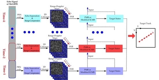
3.4. Moving Target Detection Framework

As shown in Figure 7, the moving target detection framework is presented in this section, which includes signal separation and range compression, 2D coherent processing, target detection based on the multi-Bernoulli filter, target state estimation, and target track estimation.

For an MsGBPR system, the receiver can record the echo signal continuously, as shown at the left part of Figure 7. Based on the relationship of coherent time and power budget, the slow time or coherent time T can be decided, which is also the time interval of the map. It should be noted that the time k in Section 3.2 and Section 3.3 actually means the slow time from (k − 1)T to kT. Then, for each echo signal, signal separation and range compression is performed based on the transmitter’s PRN code. As a result, the reflected echo signal from a specific transmitter can be separated and the corresponding range compression result can be also obtained. This is followed by the 2D coherent processing based on modified RFT, and multiple range-Doppler map results are then obtained. After that, depending on the quality or SNR of obtained map results, if the SNR of each map is similar, the traditional PMB filter with likelihood ratio function in (16) is implemented for target detection; on the other hand, if the map SNRs are different or unknown, the proposed modified ICMB with online SNR estimation should be adopted, and we update map results iteratively in the ascending order of map SNR. In practice, the modified ICMB filter is recommended, as the map SNR with non-cooperative targets is usually unknown. Then, the updated target density and estimated target states will be the input for the next time instant. Finally, based on the estimated target states at different time instants, targets will be detected and their tracks are also acquired.

4. Experiments and Results

To demonstrate the performance of the proposed filter and the feasibility of target detection in an MsGBPR system, numerical simulation results including online SNR estimation are provided. Signals from three GPS satellites (Space Vehicle Number, SVN #2, #10, #18) are employed. Assuming the target moves on the XOY plane, the target motion parameters and the associated simulated parameters are listed in

Table 1. Main simulation parameters.

Parameters	Values	Parameters	Values
Wavelength	0.19 m	SVN #2 Position	(−17,745.0, 1835.5, 13,077.3) km
Sampling Rate	5.0 MHz	SVN #2 Velocity	(2229.2, −519.2, 2058.0) m/s
Target Position	(140, 0, 5) km	SVN #10 Position	(10,232.9, −15,519.5, 12,420.5) km
Target Velocity	(−30, 100, 0) m/s	SVN #10 Velocity	(190.2, −2114.0, −1798.6) m/s
Map Frames	20	SVN #18 Position	(6818.7, −6090.4, 18,620.3) km
Target Appears	frame-5	SVN #18 Velocity	(1654.7, −2019.3, −926.3) m/s
Target Disappears	frame-16	SNRk,1, SNRk,2, SNRk,3	8, 9, 10 dB

. As listed, 20 maps with each transmitter are simulated, and the coherent time of each map is 2 s. The target appears at frame-5 and disappears at frame-16 with a constant velocity V (−30, 100, 0) m/s. Here the multi-transmitter index is i = 1, 2, 3, and the time series index is k = 1, 2, …, 20. The target motion is modeled by a linear stochastic process

$$x_k=F{x}_k+v_k$$

(28)

where F is the state transition matrix,

$$F=\left[\begin{array}{cccc}1& T& 0& 0\\ 0& 1& 0& 0\\ 0& 0& 1& T\\ 0& 0& 0& 1\end{array}\right]$$

(29)

With T being the frame period, and in our simulations, T = 2 s. v_k is the Gaussian distributed noise with zero mean and covariance matrix Q [29].

Map formation method in [14] is used for generating the range-Doppler map results, and the map signal model is shown in (11). The SNR_k,i is set to 8 dB, 9 dB, 10 dB, with i = 1, 2, 3 corresponding to SVN #2, #10 and #18, respectively. In order to show the range-Doppler maps with different geometric configuration, map results at frame-5, frame-10 and frame-15 using the transmitter signals SVN #2 and #10 are shown in Figure 8. It should be noted that the direct signal in the range-Doppler map has been removed [49,50]. To highlight the target, all maps in Figure 8 are noise-free. As shown in Figure 8a,d, the range history of the moving target is totally different and the target will be located in a different range-Doppler cell, if different transmitters are used. Therefore, it is really hard to fuse the range-Doppler map results directly.

To testify the effectiveness of the proposed filter for multiple transmitter signals, target detection experiments based on the set of simulated range-Doppler maps are carried out. For the SMC implementation of the modified ICMB, the birth process is a multi-Bernoulli density ${\pi }_{\mathrm{\Gamma }}=\left\{\left(r_{\mathrm{\Gamma }}^{},p_{\mathrm{\Gamma }}^{}\right)\right\}$, where only one new target is considered, $r_{\mathrm{\Gamma }}^{}$ = 0.01, and uniform distribution is used for the probability density $p_{\mathrm{\Gamma }}^{}$. The target existence probability p_s,k = 0.95, the threshold for pruning is 0.001, and a maximum of L_max = 10,000 and minimum of L_min = 2000 particles per hypothesized track are used in the simulation. The initial state of the target is generated by the uniform distribution, where x ~ U[138 km, 144 km], y ~ U[−5 km, 5 km], v_x~U[−50 m/s, −20 m/s], and v_y ~ U[80 m/s, 140 m/s].

The estimated SNR results based on the proposed online estimation method are presented in Figure 9. Based on the simulated map set above, the ideal SNR (SNR_k,i) with each transmitter is 8, 9, 10 dB, as shown by the dotted lines in Figure 9. Initially, there is no target from frame-1 to frame-4, so that the estimated SNR are just random values around 0 dB. Then, the target appears at frame-5, and the SNR of map-i is estimated. However, due to the approximation in (18), the estimation accuracy of $SN{R}_{5,i}^{ML}$ is a little bit low at the beginning. After that, with more map frames available, the estimation accuracy of $SN{R}_{k,i}^{ML}$ is gradually enhanced, especially in the high map quality case, which can be seen from the green line in Figure 9. Hence, the performance of the proposed online SNR estimation is better when the map SNR is higher. Moreover, due to the accumulated error of the likelihood ratio function among those map frames, the estimated SNR may be better than the simulated SNR in some frames. However, as shown in Figure 9, the overestimation of map SNR can be overcome as more map frames are used. From frame-16, the target disappears and the estimated SNR becomes randomly distributed again. On the whole, although the estimation accuracy of map SNR is not high at the beginning, the map SNR can be estimated effectively and it will get close to the ideal result, with more and more map frames.

Based on the estimated map SNR, the optimum update order (ascending order) is then obtained and the true target track and the estimated one in 2-D space are shown in Figure 10. At the beginning, the map SNR cannot be estimated correctly, causing errors in the modeling of the likelihood ratio function in (15). Thus, the estimated target position is far away from the true position. Then, with more frames, the estimated track becomes close to the true one gradually, demonstrating clearly the effectiveness of the proposed filter.

5. Discussion

In this section, the performance of the proposed modified ICMB filter is evaluated firstly, in terms of detection possibility, root mean square (RMS) position estimation error, and RMS velocity estimation error. Then, improvement on the efficiency of the proposed filter is presented, with tradeoff between detection efficiency and accuracy.

5.1. Performance Evaluation

With the parameters listed in Section 4, firstly, to demonstrate the importance of update strategy, the ICMB filter with both ascending and descending update strategies is used in the experiments. Here, we assume that all map SNRs are already known, so the estimation error in map SNR is avoided; for the purpose of comparison, all map SNRs are either 10 dB or 8 dB. The detected frame rate is defined to represent the detection possibility in Monte Carlo trials, which is N_d,k/N_mc, where N_d,k denotes the number of detected frame in frame-k, N_mc denotes the number of Monte Carlo trials. In our experiments, 1000 Monte Carlo trials are carried out (N_mc = 1000), and the detected frame rate results are shown in Figure 11, with a threshold of 0.5 to determine whether the target is detected or not. As shown, the target is detected when it appears (frame-5), irrespective of the update order. However, the detected frame rate in the ascending update (blue line) case is much higher than that in the descending case (red line), which verifies that the ascending update strategy should be adopted in iterated-corrector filter for multi-sensor detection. Generally, in the iterated multi-sensor filter, the overall performance of the filter will be degraded if the detection probability of the last sensor in the iterated update is low. In radar systems, the detection probability is directly related to the map quality or map SNR. Therefore, the ascending update strategy is the best in the ICMB filter. Moreover, as shown in Figure 11, the detected frame rate in both cases is higher than the case of all map SNRs being 8 dB (green line), but lower than the case of all map SNRs being 10 dB (pink line). Obviously, as expected the high SNR map provides more useful information for target detection.

To show the importance of update order in ICMB filter further, the RMS estimation error of target position and velocity is presented in Figure 12. As shown, both errors are large, but they become smaller with the increase of map frames. Same as the detected frame rate, the RMS error with ascending update order is much smaller than that with descending order, and the RMS errors for both cases are also between the two extreme cases with all-8 dB and all-10 dB map SNRs. Furthermore, as shown by the red line in Figure 12a, the final RMS error of target position in ascending update order is close to 150 m, which is an acceptable RMS position error as the range resolution of MsGBPR is expected to be around that value.

Next, the detected frame rate and RMS errors of the ICMB filter with ascending update order and the PMB filter with all map SNRs being modeled as 8 dB and 10 dB are presented. As shown in Figure 13, a missing alarm will appear if all map SNRs are modeled as 8 dB, because the map quality is underestimated; on the other hand, a false alarm also appears when all map SNRs are modeled as 10 dB, as the map quality is overestimated. Obviously, the detected frame rate and RMS error of the ICMB filter and the proposed filter are between the two extreme cases of all 8 dB and all 10 dB, as shown in Figure 13 and Figure 14. However, when the target appears initially, the performance of the ICMB filter is much better than the proposed filter r, as shown by the blue line and red line in Figure 13 and Figure 14. The reason is that the estimation accuracy of map SNR by the proposed estimation method is not high enough, which affects the order of updates and the likelihood function in (15). As shown in Figure 9, the estimation accuracy of map SNR is gradually enhanced with the increasing number of map frames. After a few frames, the map SNR is estimated more accurately, and the ascending update can be realized and the likelihood function can also be modeled accurately. Therefore, as shown by the blue line and red line in Figure 13 and Figure 14, the performance of those two filters is almost the same after a few frames, and the effectiveness and accuracy of the proposed filter are also verified.

5.2. Improvement in Computational Efficiency

For the multi-Bernoulli filter, one of the time-consuming processes is the calculation of existence probability $r_k^q$ in (8), which depends mainly on the calculation of the likelihood ratio in (15). In the MsGBPR system, the transmitted code in each GNSS satellite is the high-rate PRN sequence, which has a particularly excellent auto-correlation property. So, for the resultant range-Doppler map, the peak value and energy of side-lobe in range direction are sufficiently small. In addition, the azimuth envelope of the map is in the form of a sinc function. Therefore, the target energy is mainly concentrated in the main lobe, and the sub-area can be substituted for the whole area to calculate the likelihood ratio, which can be rewritten as

$$L_i\left(z_{k,i}|x_k,e_k\right)\approx {\displaystyle \prod _{m=1}^{N_{f\_s}}{\displaystyle \prod _{n=1}^{N_{r\_s}}\exp \left\{-\frac{{\left|g_{k,i}^{\left(m,n\right)}\left(x_k\right)\right|}^2}{{\sigma }_i^2}\right\}}}{I}_0{\left(\frac{2z_{k,i}^{\left(m,n\right)}{g}_{k,i}^{\left(m,n\right)}\left(x_k\right)}{{\sigma }_i^2}\right)}_{x_k\in X_k,z_k\in Z_k}$$

(30)

where N_{f_s} and N_{r_s} denote the size of the sub-area map in Doppler and range domains, respectively.

Experiments with different sizes of sub-area are carried out in this section. Seven different sizes are adopted for the calculation of the likelihood ratio, which are 1 × 1, 3 × 3, 5 × 5, 7 × 7, 9 × 9, 11 × 11 and the whole map size, and the corresponding performance metrics of the proposed filter are listed in

Table 2. Performance of the proposed filter with different sizes of sub-area.

	Case 1	Case 2	Case 3	Case 4	Case5	Case 6	Case 7
Nf_s × Nr_s	1 × 1	3 × 3	5 × 5	7 × 7	9 × 9	11 × 11	Nf × Nr
Power ratio	46.7%	68.9%	87.4%	94.5%	95.3%	95.6%	100%
Computation Time 1	36.86 s	38.99 s	41.33 s	43.88 s	46.65 s	50.72 s	260.05 s
Detected frame rate 2	51.9%	73.2%	95.7%	98.6%	99.4%	99.7%	99.8%

¹ The simulations are carried out on a computer with intel core i-7-6820HQ @ 2.70 GHz processors, and the programs are coded and run in MATLAB. ² Here the detected frame rate is that calculated at the last frame (frame-15) in which the target exists.

. The power ratio in Table 2 denotes the energy of the sub-area divided by the energy of the whole area. As shown, almost 90% energy is concentrated in the 5 × 5 sub-area. The corresponding computation time and detected frame rate result for different sizes of sub-area are also compared in Table 2. As anticipated, the substitution of the sub-area for the whole map to calculate the likelihood ratio will improve the computational efficiency significantly. The smaller the sub-area size is, the less the required computation time. However, substituting a single cell for the whole map to calculate the likelihood ratio improves the efficiency most, but it degrades the detected frame rate seriously. In addition, the performance degradation of detected frame rate also takes place in case 2 (3 × 3), but is negligible for other cases. Over all, the 5 × 5 sub-area is a better choice as a substitution for the whole area, with a good tradeoff between accuracy and efficiency.

6. Preliminary Experimental Results with GPS Signals

A preliminary experiment was conducted near the NanYuan Airport in Beijing, China at 14:40 (local time) on 5 January 2019, and the experimental scene is shown in Figure 15. The receiver and direct channel antenna were fixed on the grassland near the landing strip, and the receiver points to the west direction. In this experiment, a standard GPS L1 antenna was used to record the direction signal, and the GPS satellites SVN #12 and #25 are chosen as the transmitters. The illuminated moving target, an airplane, was landing from the South to the North and was around 200 m away from the receiver. More details about the experimental parameters are listed in

Table 3. Preliminary experimental parameters with GPS signals.

Parameters	Values	Parameters	Values
Wavelength	0.19 m	Satellite information	SVN # 12, #25
Signal Bandwidth	2.046 MHz	Satellite signal	L1
Sampling rate	6.2 MHz	Antenna gain	10 dB

.

With the recorded moving target echo signal, 11 frames of range-Doppler map are generated for each transmitter (SVN #12 or #25), and the time interval or coherent integration time is 0.1 s. Since the coherent integration time is very short, the airplane target can be assumed to move at a constant speed. Moreover, as the average vertical speed of airplane in a normal landing is around 2 m/s, the airplane can also be assumed to move in the XOY plane. However, as shown in Figure 16, the SNR of range-Doppler map is very low, and it will be difficult to tell whether the moving target exists directly from the range-Doppler map. In Figure 16, both the Doppler frequency caused by the satellite moving and the reference range are removed. Then, based on the proposed modified ICMB filter, the moving target detection experiment is carried out. According to the experimental scene in Figure 15, the target mainly moves in the X direction, and normally, the speed of a landing airplane is around 75 m/s. So, the initial state of the target can also be generated by the uniform distribution, where x ~ U[−200, 200 m], y ~ U[50 m, 300 m], v_x ~ U[60 m/s, 80 m/s], v_y ~ U[0 m/s, 20 m/s]. In addition, those parameters of the multi-Bernoulli filter are the same as those listed in Section 4. Using the online SNR estimation method, the estimated SNRs and measured SNRs are shown in Figure 17, and the map SNR using SVN #12 and #25 is around 11 dB and 12 dB, respectively. As demonstrated in Figure 17, the map SNR can be estimated accurately by the proposed online estimation method. So, the map using SVN #12 should be updated first during the sequential updating. In the detection experiment, the moving target is detected in 9 map frames, and it moves from frame-2 to frame-10 with the estimated speed vector being (72.4, 3.2) m/s. The main reason that the target is not detected in frame-1 and frame-11 may be due to the target being out of the receiver antenna beam. The estimated track is presented in Figure 18. The estimated speed scalar is 72.5 m/s and the estimated target range is about 200 m, which are reasonable results demonstrating again the effectiveness of the proposed modified ICMB filter.

7. Conclusions

In this paper, an MsGBPR system with a single receiver has been studied for target detection, and a modified MB filter with online SNR estimation employed as the MB filter is well suitable for low SNR applications and has good performance in multi-sensor tracking. Since the RCS of a target varies significantly with the bi-static angle or observation angle, the resultant map SNRs for different transmitters are different and both sequential updating and super-measurements updating strategies are difficult to implement in a traditional MB filter. In the proposed solution, first, the likelihood ratio function is modeled based on the range-Doppler map; based on the maximum likelihood estimation method, an online map SNR estimation method is developed using the map measurements and target signal model; then, the modified ICMB filter is proposed, which can update all measurements for multi-transmitters in the optimum order (ascending order). Furthermore, a moving target detecting framework for MsGBPR is also presented, including echo separation, 2-D coherent integration, target state estimation by the proposed method and its track generation. The excellent performance of the proposed method has been demonstrated by numerical simulations and some preliminary experimental results. Moreover, to improve the computational efficiency, a sub-area can be used as a substitute for the whole map to calculate the likelihood ratio, and based on simulation results, a 5 × 5 sub-area is recommended for the proposed method, which provides a good tradeoff between computational efficiency and detection accuracy.

Based on findings in this paper, our next work is to test the proposed method for multiple moving targets with real MsGBPR data, and later work will explore target detection using multiple receivers and multiple transmitters, as this could dramatically increase the detection performance of an MsGBPR system.

References

1. Zavorotny, V.U.; Gleason, S.; Cardellach, E.; Camps, A. Tutorial on Remote Sensing Using GNSS Bistatic Radar of Opportunity. IEEE Geosci. Remote Sens. Mag. 2014, 2, 8–45. [Google Scholar] [CrossRef] [Green Version]
2. Antoniou, M.; Cherniakov, M. GNSS-based bistatic SAR: A signal processing view. EURASIP J. Adv. Signal Process. 2013, 2013, 98. [Google Scholar] [CrossRef]
3. Cherniakov, M. Bistatic Radar: Emerging technology, Chapter 9: Passive Bistatic SAR with GNSS Transimitters; Wiley: New York, NY, USA, 2008. [Google Scholar]
4. Jin, S.; Cardellach, E.; Xie, F. GNSS Remote Sensing: Theory, Methods and Applications; Springer: New York, NY, USA, 2014. [Google Scholar]
5. He, X.; Cherniakov, M.; Zeng, T. Signal detectability in SS-BSAR with GNSS non-cooperative transmitter. IEE Proc.-Radar Sonar Navig. 2005, 152, 124–132. [Google Scholar] [CrossRef]
6. Liu, F.; Antoniou, M.; Zeng, Z.; Cherniakov, M. Coherent change detection using passive GNSS-based BSAR: Experimental proof of concept. IEEE Trans. Geosci. Remote Sens. 2013, 51, 4544–4555. [Google Scholar] [CrossRef]
7. Zeng, T.; Ao, D.; Hu, C.; Zhang, T.; Liu, F.; Tian, W.; Lin, K. Multiangle BSAR imaging based on BeiDou-2 navigation satellites: Experiments and preliminary results. IEEE Trans. Geosci. Remote Sens. 2015, 53, 5760–5773. [Google Scholar] [CrossRef]
8. Ma, H.; Antoniou, M.; Pastina, D.; Santi, F.; Pieralice, F.; Bucciarelli, M.; Cherniakov, M. Maritime Moving Target Indication Using Passive GNSS-based Bistatic Radar. IEEE Trans. Aerosp. Electron. Syst. 2018, 54, 115–130. [Google Scholar] [CrossRef]
9. Suberviola, I.; Mayordomo, I.; Mendizabal, J. Experimental Results of Air Target Detection with a GPS Forward-Scattering Radar. IEEE Geosci. Remote. Sens. Lett. 2011, 9, 47–51. [Google Scholar] [CrossRef]
10. Hu, C.; Liu, C.; Wang, R.; Chen, L.; Wang, L. Detection and SISAR Imaging of Aircrafts Using GNSS Forward Scatter Radar: Signal Modeling and Experimental Validation. IEEE Trans. Aerosp. Electron. Syst. 2017, 53, 2077–2093. [Google Scholar] [CrossRef]
11. Zeng, H.; Wang, P.; Chen, J.; Liu, W.; Ge, L. A Novel General Imaging Formation Algorithm for GNSS-Based Bistatic SAR. Sensors 2016, 16, 294. [Google Scholar] [CrossRef] [PubMed]
12. Zhou, X.; Chen, J.; Wang, P.; Zeng, H.; Fang, Y.; Men, Z.; Liu, W. An Efficient Imaging Algorithm for GNSS-R Bi-static SAR. Remote Sens. 2019, 11, 2945. [Google Scholar] [CrossRef] [Green Version]
13. Liu, F.F.; Fan, X.Z.; Zhang, L.Z.; Zhang, T.; Liu, Q.H. GNSS-based SAR for urban area imaging: Topology optimization and experimental confirmation. Int. J. Remote Sens. 2019, 40, 4668–4682. [Google Scholar] [CrossRef]
14. Zeng, H.; Chen, J.; Wang, P.; Yang, W.; Liu, W. 2-D Coherent Integration Processing and Detecting of Aircrafts Using GNSS-based Passive Radar. Remote Sens. 2018, 10, 1164. [Google Scholar] [CrossRef] [Green Version]
15. Pastina, D.; Santi, F.; Pieralice, F.; Buccciarelli, M.; Ma, H.; Tzagkas, D.; Antouiou, M.; Cherniakov, M. Maritime Moving Target Long Time Integration for GNSS-Based Passive Bistatic Radar. IEEE Trans. Aerosp. Electron. Syst. 2018, 54, 3060–3083. [Google Scholar] [CrossRef] [Green Version]
16. Chen, X.; Tharmarasa, R.; Kirubarajan, T. Multitarget Multisensory Tracking; Academic Press Library in Signal Processing, Elsevier: New York, NY, USA, 2014; pp. 759–812. [Google Scholar]
17. Mahler, R. Statistical Multisource-Multitarget Information Fusion; Artech House: Norwood, MA, USA, 2007. [Google Scholar]
18. Mahler, R. Advances in Statistical Multisource-Multitarget Information Fusion; Artech House: Norwood, MA, USA, 2014. [Google Scholar]
19. Mahler, R. Multitarget Bayes filtering via first-order multitarget moments. IEEE Trans. Aerosp. Electron. Syst. 2003, 39, 1152–1178. [Google Scholar] [CrossRef]
20. Mahler, R. PHD filters of higher order in target number. IEEE Trans. Aerosp. Electron. Syst. 2007, 43, 1523–1543. [Google Scholar] [CrossRef]
21. Vo, B.-T.; Vo, B.-N.; Cantoni, A. The cardinality balanced multi-target multi-Bernoulli filter and its implementations. IEEE Trans. Signal Process. 2009, 57, 409–423. [Google Scholar]
22. Si, W.; Zhu, H.; Qu, Z. Multi-sensor Poisson multi-Bernoulli filter based on partitioned measurements. IET Radar Sonar Navig. 2020, 14, 860–869. [Google Scholar] [CrossRef]
23. Vo, B.-T.; Vo, B.-N. Labeled random finite sets and multi-object conjugate priors. IEEE Trans. Signal Process. 2013, 61, 3460–3475. [Google Scholar] [CrossRef]
24. Vo, B.-N.; Vo, B.-T.; Phung, D. Labeled random finite sets and the Bayes multi-target tracking filter. IEEE Trans. Signal Process. 2014, 62, 6554–6567. [Google Scholar] [CrossRef] [Green Version]
25. Knoedler, B.; Broetje, M.; Koch, W. A particle filter for track-before-detect in GSM passive coherent location. In Proceedings of the IEEE Radar Conference, Boston, MA, USA, 22–26 April 2019; pp. 1–6. [Google Scholar]
26. Mallick, M.; Krishnamurthy, V.; Vo, B.-N. Track-Before-Detect Techniques in Integrated Tracking, Classification, and Sensor Management: Theory and Applications; Wiley-IEEE: New York, NY, USA, 2012; pp. 311–362. [Google Scholar]
27. Vo, B.-N.; Vo, B.-T.; Pham, N.-T.; Suter, D. Joint detection and estimation of multiple objects from image observations. IEEE Trans. Signal Process. 2010, 58, 5129–5141. [Google Scholar] [CrossRef]
28. Hoseinnezhad, R.; Vo, B.-N.; Vo, B.-T. Visual tracking in background subtracted image sequences via multi-Bernoulli filtering. IEEE Trans. Signal Process. 2013, 61, 392–397. [Google Scholar]
29. Gao, H.; Li, J. Detection and Tracking of a Moving Target Using SAR Images with the Particle Filter-Based Track-Before Detect Algorithm. Sensors 2014, 14, 10829–10845. [Google Scholar] [CrossRef] [PubMed] [Green Version]
30. Pham, N.T.; Huang, W.; Ong, S.H. Multiple sensor multiple object tracking with GMPHD filter. In Proceedings of the IEEE 10th International Conference Information Fusion, Québec, QC, Canada, 9–12 July 2007; pp. 1–7. [Google Scholar]
31. Mahler, R. Approximate multisensor CPHD and PHD filters. In Proceedings of the International Conference Information Fusion, Edinburgh, UK, 26–29 July 2010; pp. 1–8. [Google Scholar]
32. Uney, M.; Clark, D.E.; Julier, S.J. Distributed fusion of PHD filters via exponential mixture densities. IEEE J. Sel. Topics Signal Process. 2013, 7, 521–531. [Google Scholar] [CrossRef] [Green Version]
33. Guldogan, M.B. Consensus Bernoulli filter for distributed detection and tracking using multi-static Doppler shifts. IEEE Signal Process. Lett. 2014, 24, 672–676. [Google Scholar] [CrossRef]
34. Yi, W.; Jiang, M.; Hoseinnezhad, R.; Wang, B. Distributed multisensory fusion using generalised multi-Bernoulli densities. IEEE Trans. Signal Process. 2016, 11, 434–443. [Google Scholar]
35. Fantacci, C.; Vo, B.-N.; Vo, B.-T.; Battistelli, G.; Chisci, L. Robust fusion for multisensor multiobject tracking. IEEE Signal Process. Lett. 2018, 25, 640–644. [Google Scholar] [CrossRef]
36. Ong, J.; Kim, D.; Nordholm, S. Multi-sensor Multi-target Tracking Using Labelled Random Finite Set with Homography Data. In Proceedings of the International Conference on Control, Automation and Information Sciences, Chengdu, China, 24–27 October 2019; pp. 1–7. [Google Scholar]
37. Saucan, A.; Coates, M.; Rabbat, M. A Multisensor Multi-Bernoulli Filter. IEEE Trans. Signal Process. 2017, 65, 5495–5509. [Google Scholar] [CrossRef] [Green Version]
38. Vo, B.-N.; Vo, B.-T.; Beard, M. Multi-Sensor Multi-Object Tracking with the Generalized Labeled Multi-Bernoulli Filter. IEEE Trans. Signal Process. 2019, 67, 5952–5967. [Google Scholar] [CrossRef] [Green Version]
39. Yi, W.; Li, S.; Wang, B.; Hoseinnezhad, R.; Kong, L. Computationally Efficient Distributed Multi-Sensor Fusion with Multi-Bernoulli Filter. IEEE Trans. Signal Process. 2020, 68, 241–256. [Google Scholar] [CrossRef] [Green Version]
40. Kim, D.Y.; Vo, B.-N.; Vo, B.-T.; Jeon, M. A labeled random finite set online multi-object tracker for video data. Pattern Recognit. 2019, 90, 377–389. [Google Scholar] [CrossRef]
41. Nannuru, S.; Coates, M. Hybrid multi-Bernoulli and CPHD filters for superpositional sensors. IEEE Trans. Aerosp. Electron. Syst. 2015, 51, 2847–2863. [Google Scholar] [CrossRef]
42. Gostar, A.K.; Hoseinnezhad, R.; Bab-Hadiashar, A. Multi-Bernoulli sensor control via minimization of expected estimation errors. IEEE Trans. Aerosp. Electron. Syst. 2015, 51, 1762–1773. [Google Scholar] [CrossRef] [Green Version]
43. Gostar, A.K.; Hoseinnezhad, R.; Bab-Hadiashar, A. Robust multi-Bernoulli sensor selection for multi-target tracking in sensor networks. IEEE Signal Process. Lett. 2013, 20, 1167–1170. [Google Scholar] [CrossRef]
44. Nagappa, S.; Clark, D. On the ordering of the sensors in the iterated-corrector probability hypothesis density (PHD) filter. In Proceedings of the SPIE—The International Society for Optical Engineering, Orlando, FL, USA, 5 May 2011; Volume 8050, p. 80500M. [Google Scholar]
45. Mahler, R. The multisensor PHD filter: II. Erroneous solution via Poissonmagic. In Proceedings of the SPIE—The International Society for Optical Engineering, Orlando, FL, USA, 11 May 2009; p. 73360D. [Google Scholar]
46. Moreira, A.; Prats-Iraola, P.; Younis, M.; Krieger, G.; Hainsek, I.; Papathanassiou, K.P. A tutorial on synthetic aperture radar. IEEE Geosci. Remote Sens. Mag. 2013, 1, 6–43. [Google Scholar] [CrossRef] [Green Version]
47. Skolnik, M. Introduction to Radar Systems; McGraw-Hill: New York, NY, USA, 2001. [Google Scholar]
48. Olivares, J.; Martin, P.; Valero, E. A simple approximation for the modified Bessel function of zero order I 0(x). J. Phys. Conf. 2018, 1043, 012003. [Google Scholar] [CrossRef] [Green Version]
49. Fang, Y.; Atkinson, G.; Sayin, A.; Chen, J.; Wang, P.; Antoniou, M.; Cherniakov, M. Improved Passive SAR Imaging With DVB-T Transmissions. IEEE Trans. Geosci. Remote Sens. 2020, 58, 5066–5076. [Google Scholar] [CrossRef] [Green Version]
50. Garry, J.L.; Baker, C.J.; Smith, G.E. Evaluation of Direct Signal Suppression for Passive Radar. IEEE Trans. Geosci. Remote Sens. 2017, 55, 3786–3799. [Google Scholar] [CrossRef]
Figure 1. General geometric configuration of a multi-static global navigation satellite system based passive radar (MsGBPR) system.
Remotesensing 12 03495 g001
Figure 2. Diagrammatic sketch of 2-D coherent integration processing and map results in MsGBPR.
Remotesensing 12 03495 g002
Figure 3. Propagation track table in Bayesian recursive and multi-Bernoulli filter.
Remotesensing 12 03495 g003
Figure 4. Propagation track table of the product multi-Bernoulli filter.
Remotesensing 12 03495 g004
Figure 5. Propagation track table of iterated-corrector multi-Bernoulli (ICMB) filter at time k.
Remotesensing 12 03495 g005
Figure 6. Sequential Monte Carlo (SMC) implementation of the proposed modified ICMB filter.
Remotesensing 12 03495 g006
Figure 7. The proposed moving target detection framework for the MsGBPR system.
Remotesensing 12 03495 g007
Figure 8. Noise-free range-Doppler maps results: (ac) maps at frame-5, frame-10, and frame-15 with SVN#2 used; (df) maps at frame-5, frame-10, and frame-15 with SVN#10 used.
Remotesensing 12 03495 g008
Figure 9. The online estimated signal-to-noise ratio (SNR) results for SNRk,i = 8, 9, and 10 dB.
Remotesensing 12 03495 g009
Figure 10. Target detection results by the modified ICMB filter.
Remotesensing 12 03495 g010
Figure 11. Detected frame rate in different update order cases.
Remotesensing 12 03495 g011
Figure 12. Root mean square (RMS) error of target position and velocity in different update order cases: (a) RMS error of target position; (b) RMS error of target velocity.
Remotesensing 12 03495 g012
Figure 13. Comparison results of detected frame rate.
Remotesensing 12 03495 g013
Figure 14. Comparison results of RMS errors: (a) RMS error of position; (b) RMS error of velocity.
Remotesensing 12 03495 g014
Figure 15. Illustration of the experimental scene and setups.
Remotesensing 12 03495 g015
Figure 16. Experimental range-Doppler maps at frame-3: (a) SVN #12 is used as transmitter (b) SVN #25 is used as transmitter.
Remotesensing 12 03495 g016
Figure 17. The estimated SNR results using the experiment data.
Remotesensing 12 03495 g017
Figure 18. The estimated target track using the experiment data.
Remotesensing 12 03495 g018