Article

Urban Land Cover Classification of High-Resolution Aerial Imagery Using a Relation-Enhanced Multiscale Convolutional Network

1
College of Surveying and Geo-informatics, Tongji University, Shanghai 200092, China
2
Department of Compute Science, Tongji University, Shanghai 201804, China
3
Shanghai Surveying and Mapping Institute, Shanghai 200063, China
*
Author to whom correspondence should be addressed.
Remote Sens. 2020, 12(2), 311; https://doi.org/10.3390/rs12020311
Submission received: 17 December 2019 / Revised: 13 January 2020 / Accepted: 16 January 2020 / Published: 17 January 2020

Abstract

:
Urban land cover classification for high-resolution images is a fundamental yet challenging task in remote sensing image analysis. Recently, deep learning techniques have achieved outstanding performance in high-resolution image classification, especially the methods based on deep convolutional neural networks (DCNNs). However, the traditional CNNs using convolution operations with local receptive fields are not sufficient to model global contextual relations between objects. In addition, multiscale objects and the relatively small sample size in remote sensing have also limited classification accuracy. In this paper, a relation-enhanced multiscale convolutional network (REMSNet) method is proposed to overcome these weaknesses. A dense connectivity pattern and parallel multi-kernel convolution are combined to build a lightweight and varied receptive field sizes model. Then, the spatial relation-enhanced block and the channel relation-enhanced block are introduced into the network. They can adaptively learn global contextual relations between any two positions or feature maps to enhance feature representations. Moreover, we design a parallel multi-kernel deconvolution module and spatial path to further aggregate different scales information. The proposed network is used for urban land cover classification against two datasets: the ISPRS 2D semantic labelling contest of Vaihingen and an area of Shanghai of about 143 km2. The results demonstrate that the proposed method can effectively capture long-range dependencies and improve the accuracy of land cover classification. Our model obtains an overall accuracy (OA) of 90.46% and a mean intersection-over-union (mIoU) of 0.8073 for Vaihingen and an OA of 88.55% and a mIoU of 0.7394 for Shanghai.

Graphical Abstract

1. Introduction

Urban land use and land cover information is essential for understanding the constant changes on the surface of the Earth and associated socioecological interactions [1]. This information has great value for land resource management, urban environment monitoring, change detection, and nature conservation [2,3,4]. With advances in remote sensing data acquisition technologies, a huge amount of remote sensing images with high spatial resolution are steadily becoming more widespread [5,6]. This opens new opportunities for urban land cover information extraction at a very detailed level [7]. However, the manual interpretation of such massive and complex images is time-consuming and labor-intensive. Hence, it is urgent to interpret high-spatial-resolution remote sensing images in intelligent and automatic methods for land cover classification [8,9].
Automatic urban land cover classification in remote sensing images is a difficult task due to several challenges. First of all, high-resolution remote sensing images with abundant details generally have characteristics of high intraclass variance and low inter-class variance [10]. For example, different classes of ground objects may have a similar appearance in remote sensing images, such as trees and low vegetation or roofs and roads. Meanwhile, there is occlusion between different objects. To solve this issue, context information has been widely studied in remote sensing image classification [11]. Contextual information refers to the dependencies between objects, such as cars on roads. Misclassification will be reduced when taking these context relationships into account. In addition, ground objects often have various scales in remote sensing images. Cars and buildings have large differences in size. It is difficult to simultaneously distinguish objects with distinct scales. Generally, deeper layers with larger receptive fields are more suited for segmenting large objects, while shallower layers with smaller receptive fields are suitable to segment small objects [12]. Therefore, it is necessary to enhance global context relationships and fuse multiscale information for pixel-level classification.
Recently, methods based on the fully convolutional network (FCN) [13] have been proposed to solve the above problems. The most common strategies fuse multiscale context relationships. One method makes use of the various dilation rate convolutions or pyramid pooling operations to aggregate multiscale context information [14,15,16]. Another method uses a large kernel size and combines features from different stages of the network to capture long-range information [17,18]. To further recover feature map spatial information, the encoder–decoder architecture is proposed to aggregate different levels’ features [19,20,21]. Although context fusion considers different-scale objects, it ignores long-range context relationships between objects. This may lead to intraclass inconsistency and affect the segmentation accuracy. Moreover, most approaches need abundant labeled training samples to avoid overfitting, while the sample size is relatively small in the remote sensing field because the cost of labelling extensive samples is very expensive. To save computing resources and achieve better feature representations, an attention mechanism based on methods was employed to capture contextual information for image classification [22,23]. The attention mechanism can take the initiative to focus on some key regions and aggregate them to enhance feature representations. For instance, Mou et al. [23] used the recurrent network to process the pixels of hyperspectral images via a sequential perspective for capturing the intrinsic relationships. However, the attention mechanism based on the recurrent neural network needs repeated operations to capture long-range dependencies. This characteristic leads to difficulties for network optimization [24].
To address the above issues, this study proposed a relation-enhanced multiscale convolutional network (REMSNet) for urban land cover classification, as shown in Figure 1. The proposed network architecture is based on DenseNet [25], which encourages feature reuse and thus remarkably reduces the number of parameters while maintaining good performance. In addition, the inception module [26] is adopted in the initial encoding stage to alleviate contradictions between multiscale objects and fixed receptive fields. Then, we introduce relation-enhanced blocks to capture global context relations in the spatial and channel domains. The spatial relation-enhanced block uses a weighted sum of the features at all positions to generate spatial relation-augmented feature representation. The weight depends on the semantic similarities between the two positions. The channel relation-enhanced block is applied to adaptively strengthen the channel-wise features through modeling relationships between channels. Finally, the parallel multi-kernel deconvolution module and spatial path are designed in the decoding stage to further extract features simultaneously at several scales and aggregate local and contextual information. The main contributions of our paper are as follows:
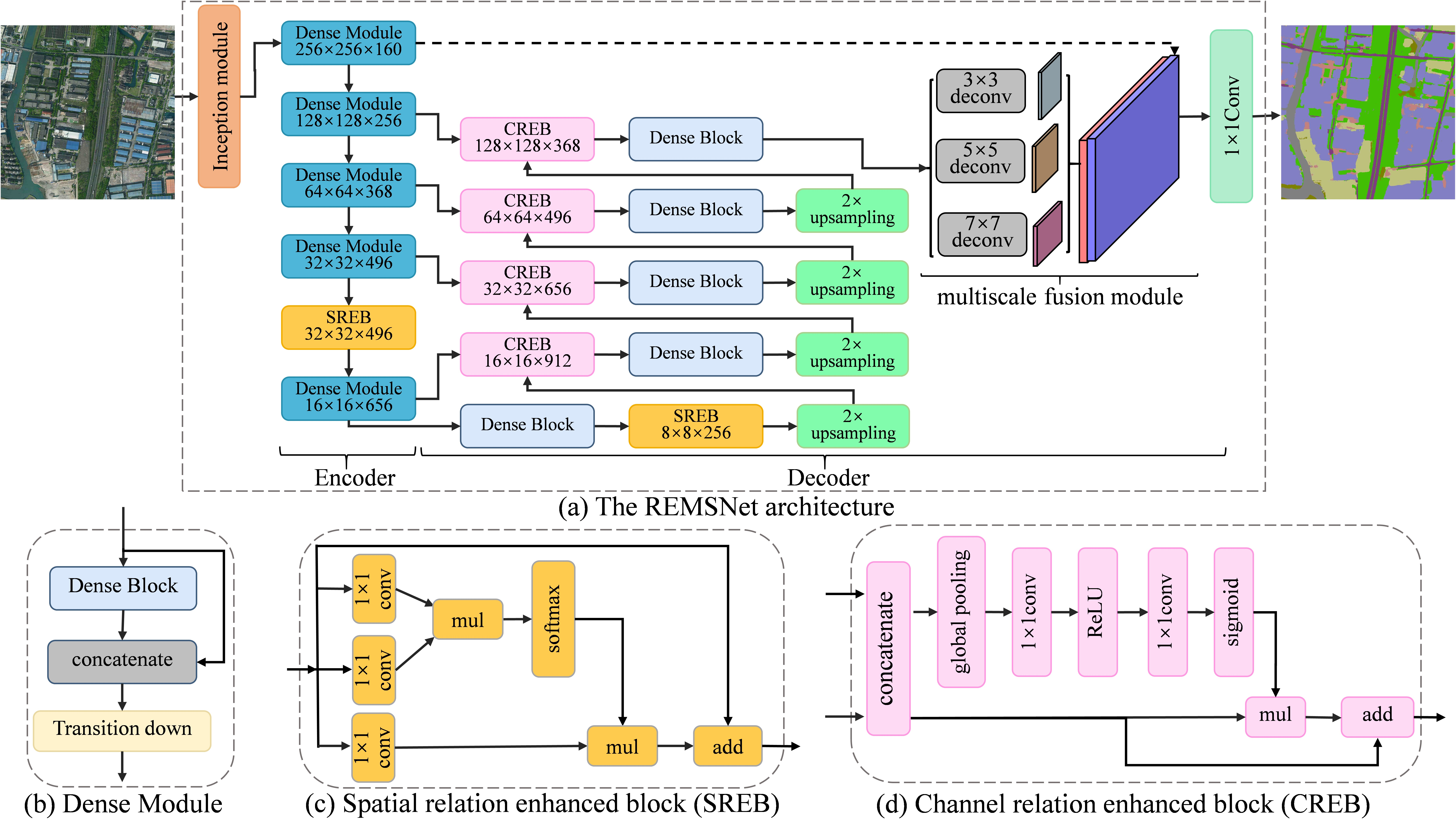
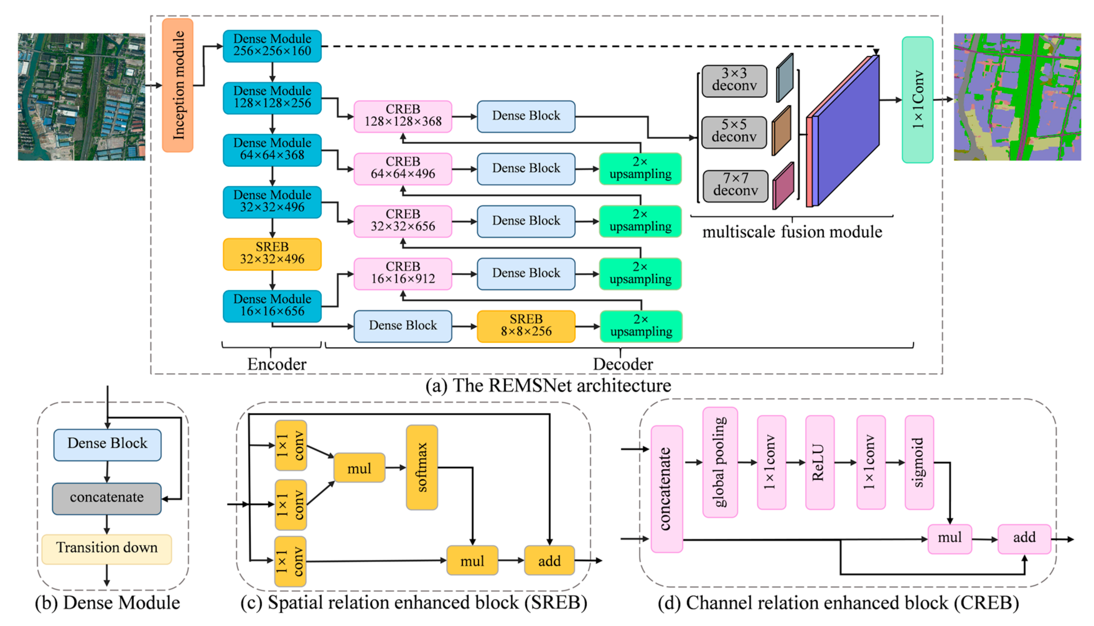
  • The proposed network uses a dense connectivity pattern to build the lightweight model. Meanwhile, parallel multi-kernel convolution and deconvolution modules are designed in the encoding and decoding stages, respectively, to increase the variety of receptive field sizes that can capture different scales objects more effectively.
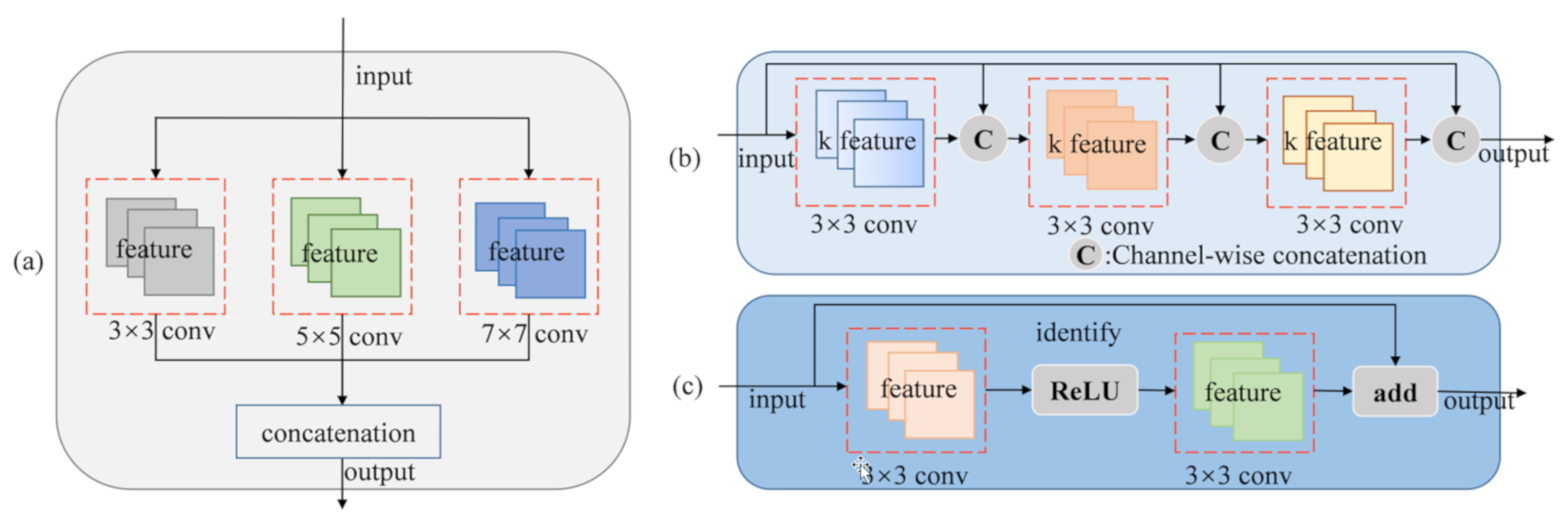
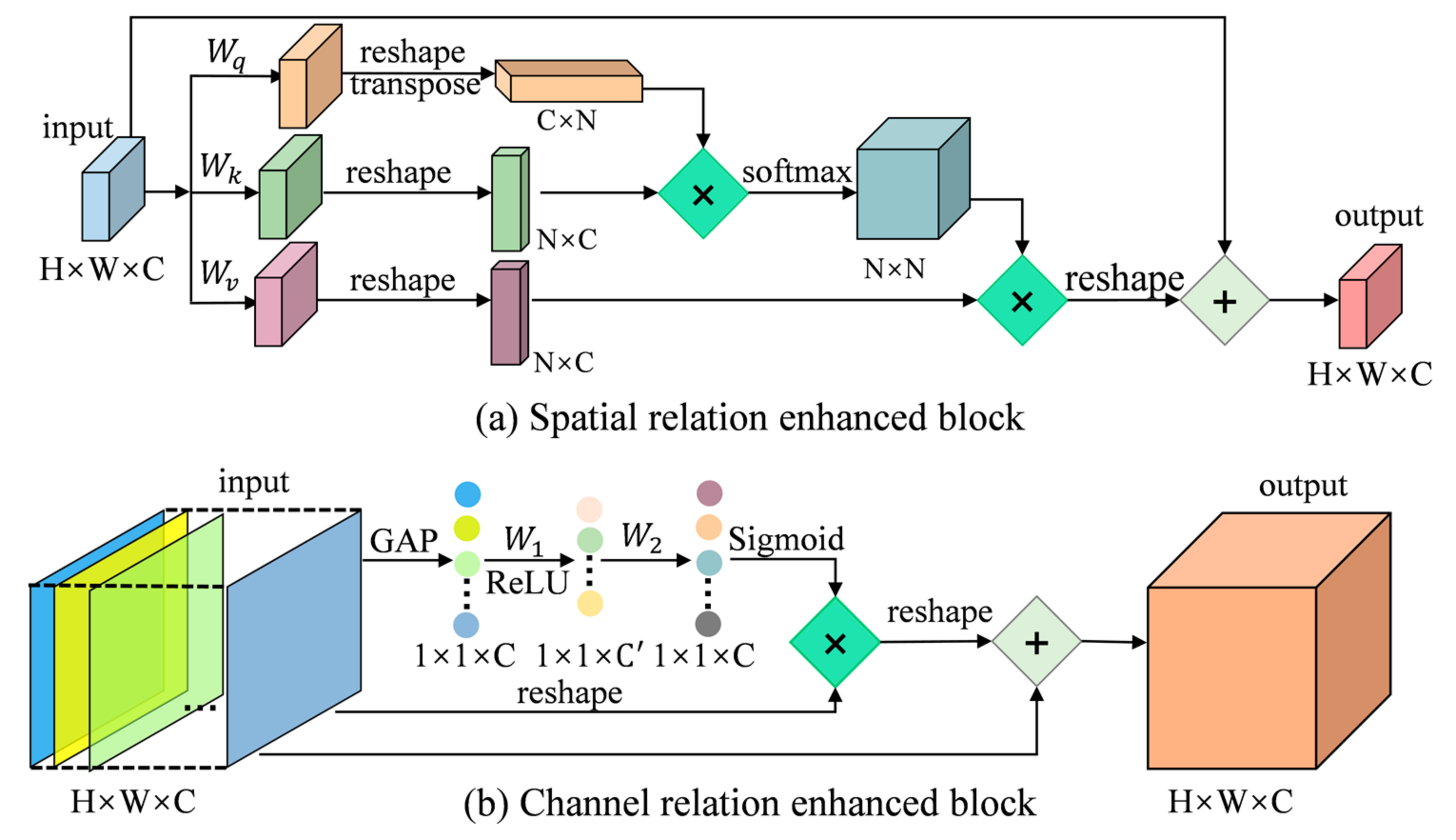
  • We introduce spatial and channel relation-enhanced blocks to explicitly model spatial and channel context relationships. They significantly improve the classification results by capturing global context information in the spatial and channel domains.
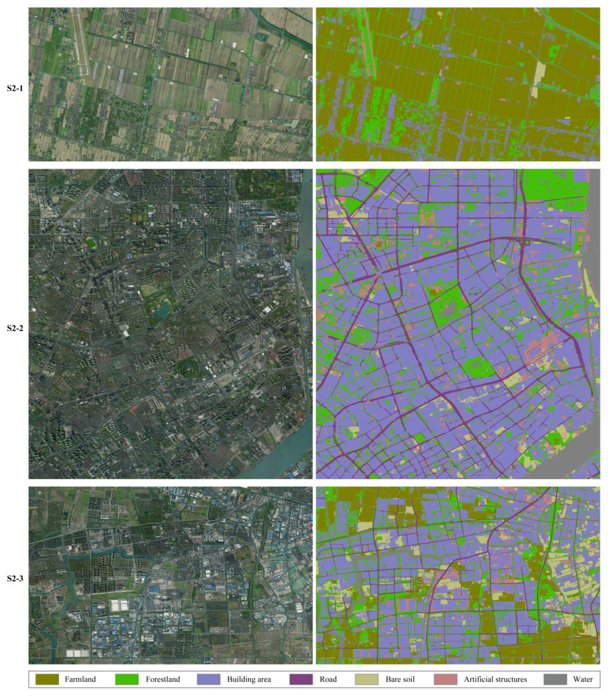
  • We propose a relation-enhanced multiscale network for urban land cover classification in aerial imagery. Case studies with the ISPRS Vaihingen dataset and an area of Shanghai of about 143 km2 demonstrate that the proposed REMSNet can generate a better land cover classification accuracy and can produce more practical land cover maps compared with several state-of-the-art deep learning models.
The remainder of this paper is organized as follows: Section 2 discusses related work on deep learning. Section 3 describes details of our network structure. The experimental results of the classification and analysis are presented in Section 4, followed by a discussion in Section 5. The conclusions are outlined in the last section.

2. Related Work

Dense pixel-wise classification is also called semantic segmentation in computer vision. Recently, semantic segmentation based on deep learning has been widely used in both computer vision and remote sensing areas. There are many detailed review papers on this topic [4,27,28]. In this section, relevant works on high-resolution aerial imagery classification/semantic segmentation and the attention mechanism are briefly reviewed.

2.1. Semantic Segmentation for High-Resolution Aerial Images

Models based on FCN have demonstrated significant improvements on several remote sensing segmentation benchmarks. Sherrah [10] proposed a no-downsampling approach to maintain the full resolution of the feature map at every layer based on a pretrained FCN. Sun Weiwei et al. [29] introduced the maximum fusion strategy into FCN to combine semantic information from deep layers and detailed information from shallow layers. Despite the power and flexibility of the FCN model, its inherent spatial invariance does not take into account useful global context information [27]. Currently, various model variants are proposed to capture the contextual information, including aggregating multiscale context information or using graph model-based methods.
In order to fuse mutiscale context information, Yu et al. [16] designed an improved version of Pyramid Scene Parsing Network (PSPNet) [30] to extract multiscale features for high-resolution aerial images semantic segmentation. Panboonyuen et al. [17] modified the global convolutional network (GCN) [18] to further enhance the ability of extracting multiscale features from different stages of the network. However, those methods may result in a low spatial resolution segmentation result, in which class boundaries become blurry. To recover a certain extent of spatial information, the encoder–decoder architecture has been designed, such as U-Net [21] and SegNet [31]. Typically, the encoder module gradually downsamples and captures higher semantic information and the decoder module gradually recovers the spatial information [15]. Liu et al. [19] introduced skip connections with residual units and an inception module in an hourglass-shaped encoder–decoder structure to improve the segmentation accuracy of remote sensing images. Sun et al. [32] concatenated two U-Nets to allow multiple outputs for road extraction from high-resolution images. To explicitly represent class boundaries, Marmanis et al. [33] added boundary detection to the SegNet to further refine classification results. Liu et al. [34] introduced multiple weighted edge supervisions based on the encoder–decoder framework to leverage the spatial boundary context and reduce the semantic ambiguity. Some work also uses multi-source data fusion data to reduce ambiguous boundary. Audebert et al. [35] studied how to implement an efficient multiscale neural network using SegNet and ResNet [36] for dealing with multi-modal and multiscale remote sensing data. Sun et al. [37] designed a parallel multi-filter encoder-decoder structure and multi-resolution segmentation to aggregate light detection and ranging (LiDAR) data and high-resolution optical imagery and reduce salt-and-pepper artifacts.
Graph model-based methods are also an available way to obtain contextual information such as conditional random fields (CRFs). CRFs are generally used in postprocessing to refine spatial details [38]. Among those methods, CRFs only optimize the segmentation results and do not participate in the training process of the network. Some studies make CRFs differentiable [39] or turn them into a recurrent network [40] to train with the network end-to-end. He et al. [41] integrated a skip-connected encoder–decoder network structure and CRF layer to implement end-to-end network training, and the result was improved by taking more information into account. To reduce salt-and-pepper noise, Zhao et al. [11] transformed image pixel labels into semantic segments and presented a semantic segment-based CRF method to effectively exploit the contextual relationships between different categories of ground objects. However, these methods need iterative inference processes, which is a time-consuming operation.
In this work, we extend the encoder–decoder architecture to the task of land cover classification. The dense connectivity pattern and attention mechanism are introduced to the encoder–decoder architecture to better capture global contextual relations and fuse different levels of the feature map while keeping the network lightweight.

2.2. Attention Mechanism

Attention mechanism-based methods have become a powerful tool to capture long-range dependencies in neural networks [24,42,43]. They play an important role in many tasks including machine translation, image captioning, and video classification. Generally, attention methods are designed to calculate the representation of each position by a weighted sum of the features at all positions [44]. Bahdanau et al. [42] proposed an attention method that emphasizes the most relevant words in a source sentence when predicting a target word. Wang et al. [24] proposed a non-local operation as a lightweight and general block to capture long-range dependencies for video classification. PSANet [45] used the point-wise spatial attention to relieve the local neighborhood constraint, and a self-adaptively learned attention mask was designed to connect each position on the feature map to all the other ones. Motivated by the above attention methods, Yuan et al. [46] introduced an object context pooling (OCP) scheme to represent each pixel by exploiting the set of pixels that belong to the same object category with such a pixel.
In order to incorporate multiscale features into deep neural networks, Chen et al. [47] jointly trained the network and an attention model which weights the relevant features pixel-by-pixel at different positions and different scales. Pyramid attention network (PAN) [43] introduced a spatial pyramid attention structure to fuse different scale contextual information and produce better pixel-level attention for high-level feature maps. Previous literature has also focused instead on the channel dependencies. Hu et al. [48] modelled channel relationships by a Squeeze-and-Excitation block, which uses global average pooling to compute channel-wise attention. Sanghyun et al. [49] improved the Squeeze-and-Excitation block and proposed a Convolutional Block Attention Module to sequentially infer attention maps from channel and spatial dimensions.
Inspired by recent advances in attention approaches, we introduce the spatial relation-enhanced block to strengthen the local features via aggregating information from other positions in the coding stage. In the decoding stage, channel relation-enhanced blocks are designed to learn long-range dependencies in the channel domain.

3. The Proposed Network

For urban land cover classification from high-resolution aerial images, the relation-enhanced multiscale convolutional network is proposed in this work. Figure 1 shows the overview architecture of the proposed network. We first illustrate how to construct our network architecture based on existing methods in the literature. Then, we describe the main principles of the spatial relation-enhanced block and channel relation-enhanced block, which can enhance context relations among diverse ground objects. Finally, the details of the multiscale fusion module are described, including the multi-kernel deconvolution feature fusion module and spatial path design.

3.1. Proposed Network Architecture

Inspired by the encoder–decoder architecture [19], the proposed network architecture mainly comprises a downsampling path (encoder) and an upsampling path (decoder), as shown in Figure 1a. The encoder is designed to capture abundant semantic information. Our encoder backbone adopts the idea from DenseNet [25], which uses a dense connectivity pattern to promote the different levels of feature reuse and significantly reduces the number of parameters while increasing performance. Since local receptive fields may cause intraclass inconsistency and affect the segmentation accuracy, parallel multi-kernel convolutions and spatial relation-enhanced blocks (Figure 1c) are also introduced in the encoder to increase receptive fields and capture global contextual information. The decoder uses upsampling layers to gradually recover the spatial information. Meanwhile, the decoder uses channel relation-enhanced blocks (Figure 1d) which can learn long-range dependencies in the channel domain to selectively emphasize key features and suppress less useful ones. To aggregate multiscale features effectively, a multiscale fusion module is designed at the end of the decoder.
The encoder, as a feature extractor, is of vital importance as its structure directly affects the speed, accuracy, and memory of the classifier. The traditional CNN adopting fixed kernel sizes limits observation scales [37], so the first part of our encoder is the simplified inception module, as illustrated in Figure 2a. The inception module [26] consists of parallel convolutional layers with different kernel sizes (3 × 3 convolution, 5 × 5 convolution, 7 × 7 convolution). This design makes various receptive fields in each of the parallel paths, which increases the width and depth of a network. Moreover, this model can capture and aggregate features at multiple scales. Then, those features input the dense module. Their design principle is to connect each layer to every other layer in a feed-forward way. Unlike traditional convolutional networks, where L layers have L connections, the dense module has L(L2 + 1)/2 direct connections. This connectivity pattern improves the information flow between layers and makes the network easy to be trained [25]. The dense module is composed of dense blocks and pooling operations. Each dense block connects each layer to all the previous layers, as shown in Figure 2b. Therefore, the output of the l layer is defined as
x l = F x 0 , x 1 , , x l 1 ,
where x 0 , x 1 , , x l 1 is the concatenation of the feature maps produced in layers 0,…, l − 1, l; F(.) represents every layer in the dense block operations, which are the following operations: batch normalization (BN) [50], then a rectified linear unit (ReLU), 3 × 3 convolution (Conv) with dropout = 0.2. Note that a 3 × 3 convolution needs a padding operation to ensure all feature maps are the same size in the dense block. Every layer in the dense block has a fixed number of convolutional filters (growth rate k). Pooling operations consist of a 1 × 1 convolution followed by a 2 × 2 average pooling layer. Finally, the spatial relation-enhanced block is introduced to capture global dependencies after the dense module.
The decoder part is used to recover and aggregate different feature maps extracted by the encoder path. Combining different resolutions and scales of feature maps can improve the segmentation performance [14,16]. Accordingly, our decoder is composed of upsampling layers, the channel relation-enhanced block, and the multiscale fusion module. Upsampling layers use deconvolution to recover the feature map resolution. Meanwhile, channel relation-enhanced blocks are used to capture the global context information when recovering the information from semantic feature maps with low spatial resolution. In order to further combine different sizes of spatial context information, the multiscale fusion module is designed at the end of the encoder. The details of the channel relation-enhanced block and multiscale fusion module are described in Section 3.3 and Section 3.4.

3.2. Spatial Relation-Enhanced Block

Capturing and utilizing global contextual information is of critical importance for semantic segmentation [51]. However, local features generated by general fully convolutional networks could result in misclassification [18,30]. In order to obtain long-range spatial relations over local features, we introduce the spatial relation-enhanced block. The spatial relation-enhanced block strengthens the local features via aggregating information from other positions, thus enhancing the network ability of feature representation.
The structure of the spatial relation-enhanced block is shown in Figure 3a. Given a feature map X = [ x 1 x 2   , x 3   ,…,   x N   ] as input, where x i   ∈ R1×1×C is feature-map vector at spatial positions i, and N = H × W represents the number of all positions in the feature map, X ˜ denotes spatial relation-enhanced feature maps, which have the same channels as X. The spatial relation-enhanced block can then be expressed as:
x ˜ i = x i + j = 1 N f x i , x j X g x j ,
where f x i , x j denotes relationships between vectors x i and x j   , X is a normalization factor. Therefore, f x i , x j / X represents normalized relationships between vectors x i and x j   . g x j = W v x j represents linear transform matrices. W v implements the 1 × 1 convolution in this block. The embedded Gaussian is used as f x i , x j in our model, which calculates the similarity in an embedding space, defined as:
f x i , x j X = exp m x i ,   n x j i = 1 N exp m x i ,   n x j ,
where m x i and n x j denote the linear transform matrices: m x i = W q x i   , n x j = W k x j   . W q and W k implement the 1 × 1 convolution in this block.
The block establishes relationships between two arbitrary spatial positions, which allow for similar semantic features to contribute to mutual improvement. The enhanced features have global context information and selectively aggregate contexts according to their calculated relationships. Meanwhile, the block has a flexible form. It can be easily inserted into the network to combine both global and local information.

3.3. Channel Relation Enhanced Block

Each channel of the high-level feature maps can be taken as a specific category of response, because they have strong semantic information [48]. However, high-level features lack basic spatial information, which is not conducive for accurate boundary localization. Low-level features have finer spatial information, but they have poor semantic information because of their small receptive view. We can exploit the interdependencies between high- and low-level channel maps to improve the feature representation of specific semantics. Therefore, the channel relation-enhanced block is introduced to definitely model the relationships among channels of different-level feature maps.
As illustrated in Figure 3b, we first use global average pooling (GAP) to generate global context information from each channel of the feature map. Given a feature map V= v 1 , v 2 , v 3 , , v C   ,
u z = F GAP v z = 1 H × W i = 1 H j = 1 W v z i , j ,
where v z R H × W denotes the z-th channel of the V, C is the total numbers of channels, and u z denotes the z-th channel squeezing global information.
Then, a gating mechanism with sigmoid activation is used in this block for highlighting class-relevant channel relations and suppressing irrelevant channel dependencies [17,48]. To reduce the computational and model parameters, we add linear transform matrices around the activation:
s z = F s u , W = Sigmoid W 2 . ReLu W 1 . u Z ,
where W 1 and W 2 represent 1 × 1 convolution. F s u ,   W can obtain the different weights of each channel by training. The final channel relation-enhanced feature maps V ˜ are as follows:
v ˜ z = F r v z , s z = v z + v z × s z ,
where V ˜   = v ˜ 1 , v ˜ 2 , v ˜ 3 , , v ˜ C denotes channel relation-enhanced feature maps, and × refers to channel-wise multiplication.
The channel relation-enhanced block makes use of channel relations establishing weights to different levels of features; thus, class-relevant features can be assigned more weights adaptively.

3.4. Multiscale Fusion Module

Multiscale feature fusion has been proven to be effective for remote sensing image classification [14]. Therefore, multi-kernel deconvolution is designed at the end of our network to extract features simultaneously at several scales and aggregate that information. This module has three parallel deconvolutions with kernel sizes of 3 × 3, 5 × 5, and 7 × 7, while using a padding operation makes the size of the feature maps the same. Then, the average values of different-scale features are obtained. Given a feature map X as input, Z denotes integration features:
Z = 1 S s = 1 S W s X ,
where S is the number of different kernels or scales, and W S denotes the convolutional kernel for the input map X at scale s. Different kernel sizes make it possible to integrate different-scale context information step-by-step. This module can combine different receptive field features and consider different sizes of spatial context information effectively.
Spatial information is important to predict the detailed outputs in the semantic segmentation task [52]. However, consecutive downsampling operations may result in the loss of some spatial information. Inspired by the BiSeNet [52], a spatial path is designed to further preserve the spatial information and obtain high-resolution features, as shown in Figure 1a. Finally, the spatial feature map and multi-kernel feature map are fused to predict outputs.

4. Experimental Results and Analysis

To evaluate the classification performance of our network, we conducted urban land cover classification experiments on two datasets: the ISPRS 2D semantic labelling contest of Vaihingen and an area of Shanghai of about 143 km2. Visual inspection and quantitative accuracy assessment, with overall accuracy (OA), mean intersection-over-union (mIoU), and F1 score, were adopted to evaluate the classification results. Furthermore, the performance of our network was compared with typical land cover classification methods based on deep learning.

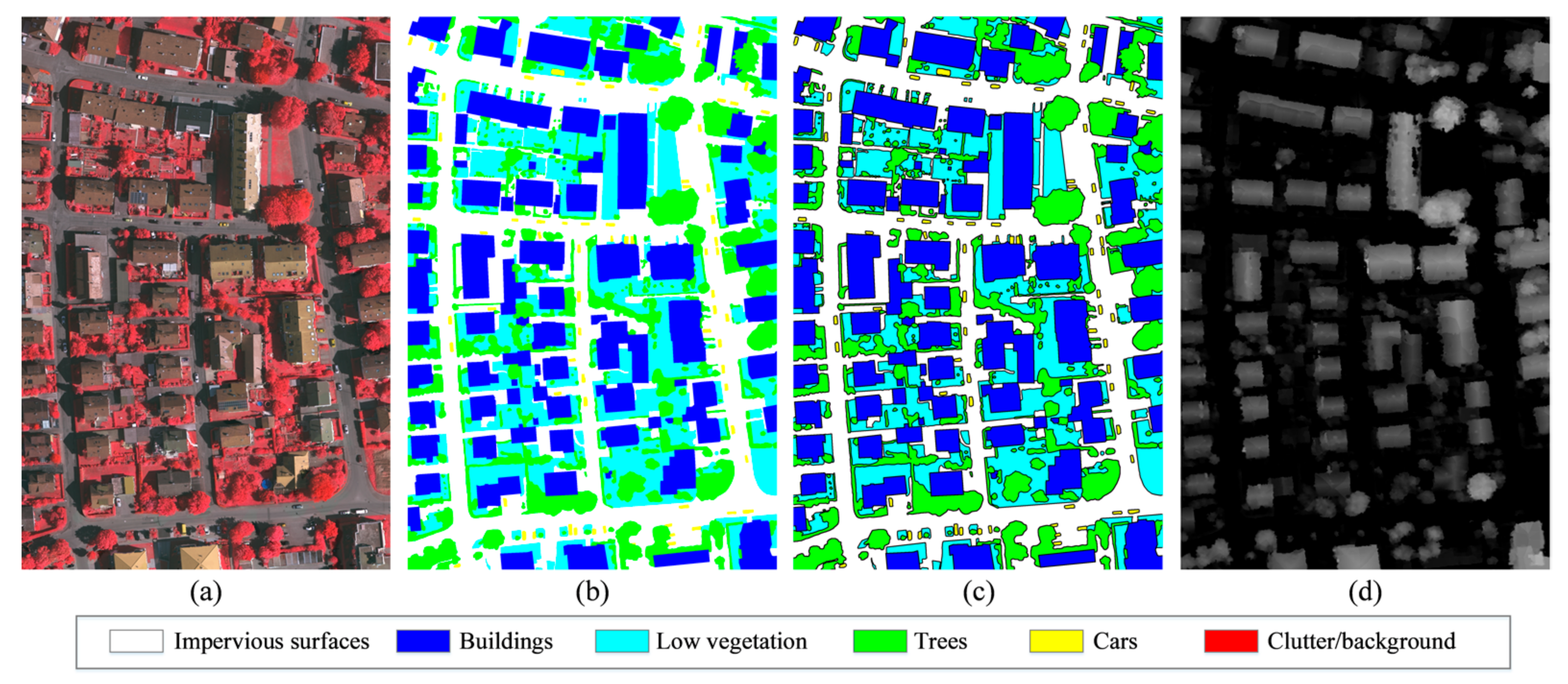
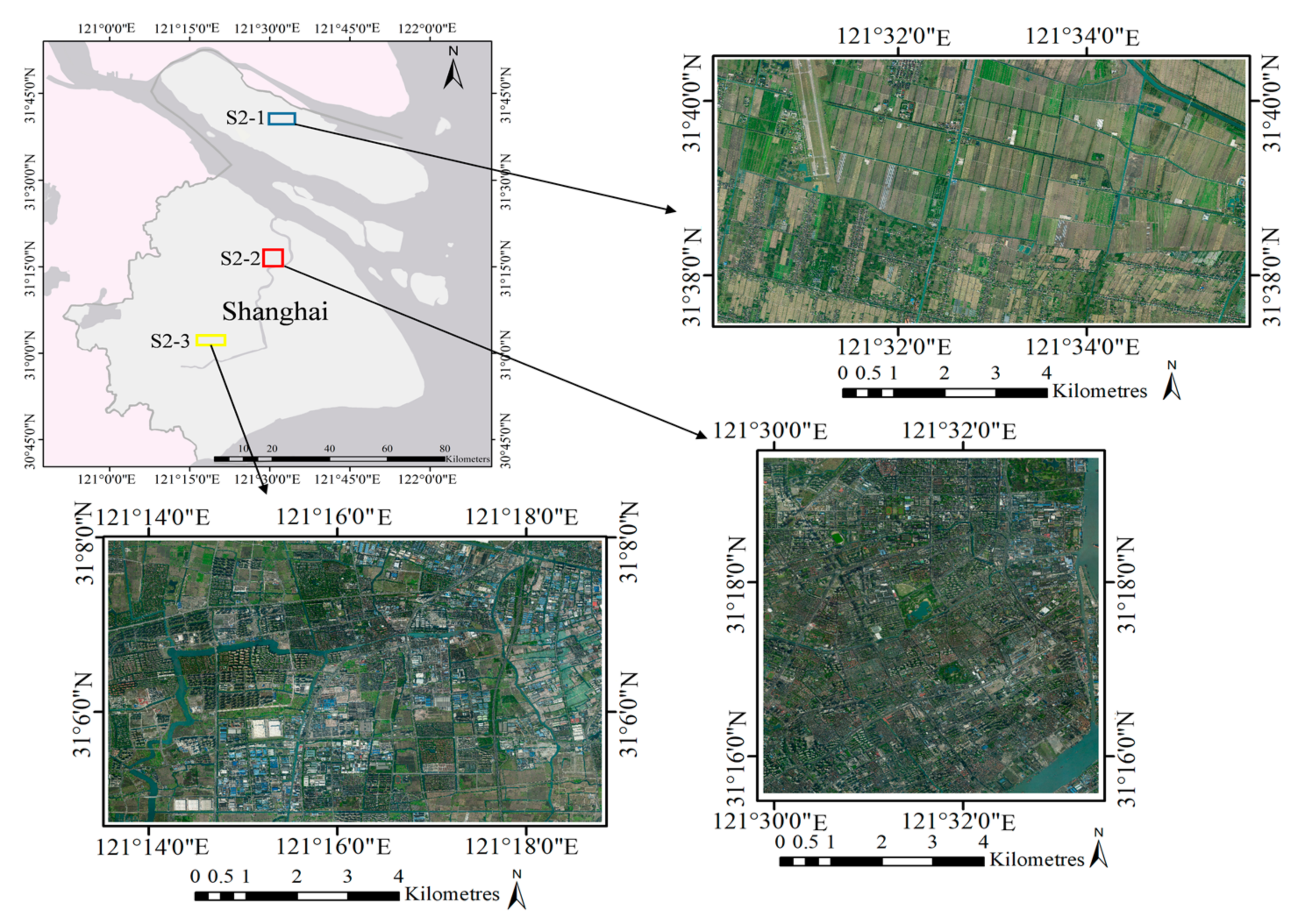
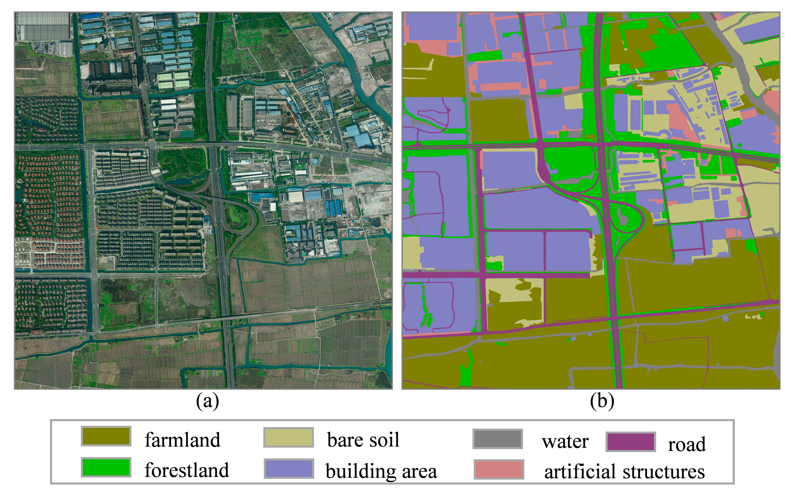
4.1. Study Area and Preprocessing

4.1.1. Study area and data description

Study area I is located in in Vaihingen, Germany. It is a relatively small town with many detached buildings and small multi-story buildings [53]. This is a benchmark dataset for aerial image classification provided by the ISPRS 2D Semantic Labeling Challenge [53]. The Vaihingen dataset consists of 33 image tiles with an average size of 2494 × 2064 and a spatial resolution of 9 cm. Among them, only 16 images have ground truth. Each image has three bands, corresponding to near infrared (NIR), red (R), and green (G). The dataset also provides a Digital Surface Model (DSM) corresponding to the image tiles. The Normalized Digital Surface Model (nDSM) provided by Gerke et al. [54] is used in our experiments. Six categories were defined in the dataset including impervious surfaces, building, low vegetation, tree, car, and clutter/background, as shown in Figure 4. We selected five images (image IDs: 11, 15, 28, 30, 34) to evaluate our network; the remaining images were used for training, following the procedure in [19,34,54,55,56]. To reduce the impact of uncertain border definitions, another version of the ground truth with eroded boundaries is provided, on which the accuracy is measured [19,34,54,55,56]. In these images, boundaries between classes are eroded with a disk radius of three pixels. In this study, our model ignores the category of clutter/background, due to the minority sample distribution among the training tiles.
Study area II is located in Shanghai, China. Shanghai has a complex spatial distribution and various types of land use. This is necessary for the automatic classification of land cover. Moreover, land cover classification can better understand and analyze cities. Three areas were selected for experimentation, namely Chongming (S2-1), Yangpu (S2-2), and Qingpu (S2-3) and their surrounding regions, as shown in Figure 5. The study sites are located in rural, central urban, and suburban areas that are highly heterogeneous and distinctive from each other in both spatial arrangement and the types of land cover. Therefore, the areas are suitable for evaluating the generalization ability of the network. Aerial images were acquired on 17 May 2017. The images have three channels (Red, Green, Blue) with a spatial resolution of 0.5 m. Their spatial extents are 19,110 × 10,351 pixels for S2-1, 12,139 × 13,152 pixels for S2-2, and 17,863 × 11,055 pixels for S2-3. The Shanghai dataset had to be labelled before use, and the Shanghai Surveying and Mapping Institute labelled those aerial images based on existing geodatabases. Seven classes were defined among S2-1, S2-2, and S2-3 comprising building area, road, farmland, forestland, bare soil, artificial structures, and water (Figure 6). In our experiment, six images were selected to evaluate our network, including four images (5983 × 4255 pixels) from S2-1, S2-2 and two images (7320 × 4902 pixels) from S2-3. The remaining images were used for training.

4.1.2. Data Preprocessing and Augmentation

Due to the limited memory of Graphics Processing Unit (GPU), each remote sensing image was cropped into smaller patches of size 400 × 400 pixels, using a sliding window. All patches were normalized to [0,1] to expedite the network convergence speed in training. Previous works [25,26] indicate that data augmentation is an effective way to virtually enlarge the training dataset size and improve the generalization ability of the network. Our training datasets are relatively small to train the proposed network, especially in the Vaihingen dataset. Therefore, following data augmentation techniques were used to increase the diversity and quantity of the training set. When training networks, each image with a size of 400 × 400 pixels was sliced into a subimage of 256 × 256 pixels randomly. Moreover, we further increased the training samples through random vertical and horizontal flips in the training progress.

4.2. Training Detail and Evaluation Metrics

All the networks were implemented based on the deep learning framework Tensorflow [57]. All experiments were on a Dell workstation with an Intel Xeon E5-2630 v3 CPU, NVIDIA GTX-1080Ti GPU (11 GB memory) and 32 GB RAM. The workstation operating system is Ubuntu 16.04. Specifically, a pretrained ResNet101 [36] was used as a backbone for deeplabv3 and PSPNet. The RMSprop [58] optimizer was utilized to optimize our networks, which operates at an initial learning rate of 0.001 and an exponential decay of 0.995 after each epoch. We trained the network using a batch size of 1 for 300 epochs. For the Vaihingen dataset, spectral information (NIR-R-G) and the nDSM were used as the network input. The input size was 256 × 256 pixels. For the Shanghai dataset, the network input was RGB images with a size of 256 × 256 pixels.
To assert the performance of the land cover classification, the confusion matrix, overall accuracy (OA), mean intersection-over-union (mIoU), and F 1 score ( F 1   ) were used. The main metrics are defined as follows:
F 1 = 2 × precision × recall precision + recall ,
OA =   TP N ,  
  IoU = TP TP + FP + FN ,  
where
precision   =     TP TP + FP   recall   =     TP TP + FN ,  
where TP is true positive, FP is false positive, FN is false negative, and N is the total pixel number.

4.3. Results and Analysis

In this section, we show the extensive experimental results obtained with the proposed method and other typical deep learning models for semantic segmentation, including SegNet [31], MobileNet [59], deeplabv3 [15], FC-DenseNet [50], and PSPNet [30]. In addition, our method was compared with other published research on the same dataset as well.

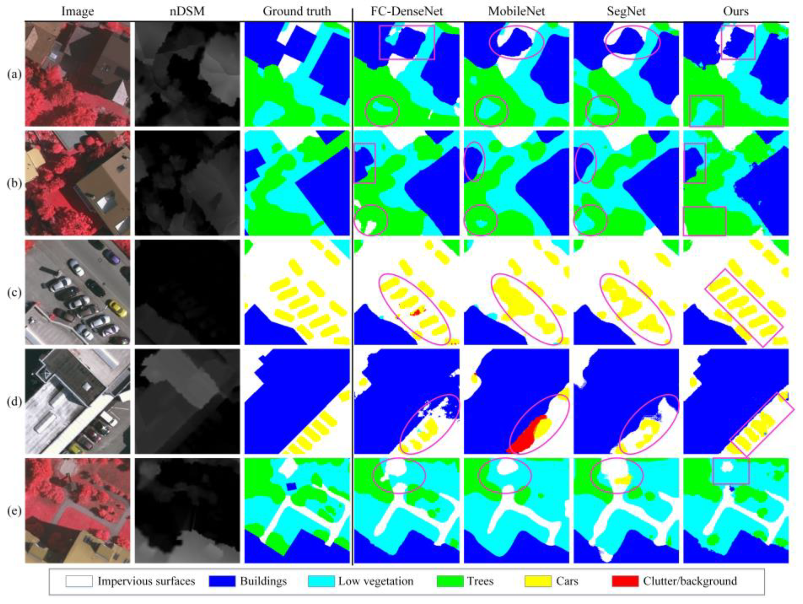
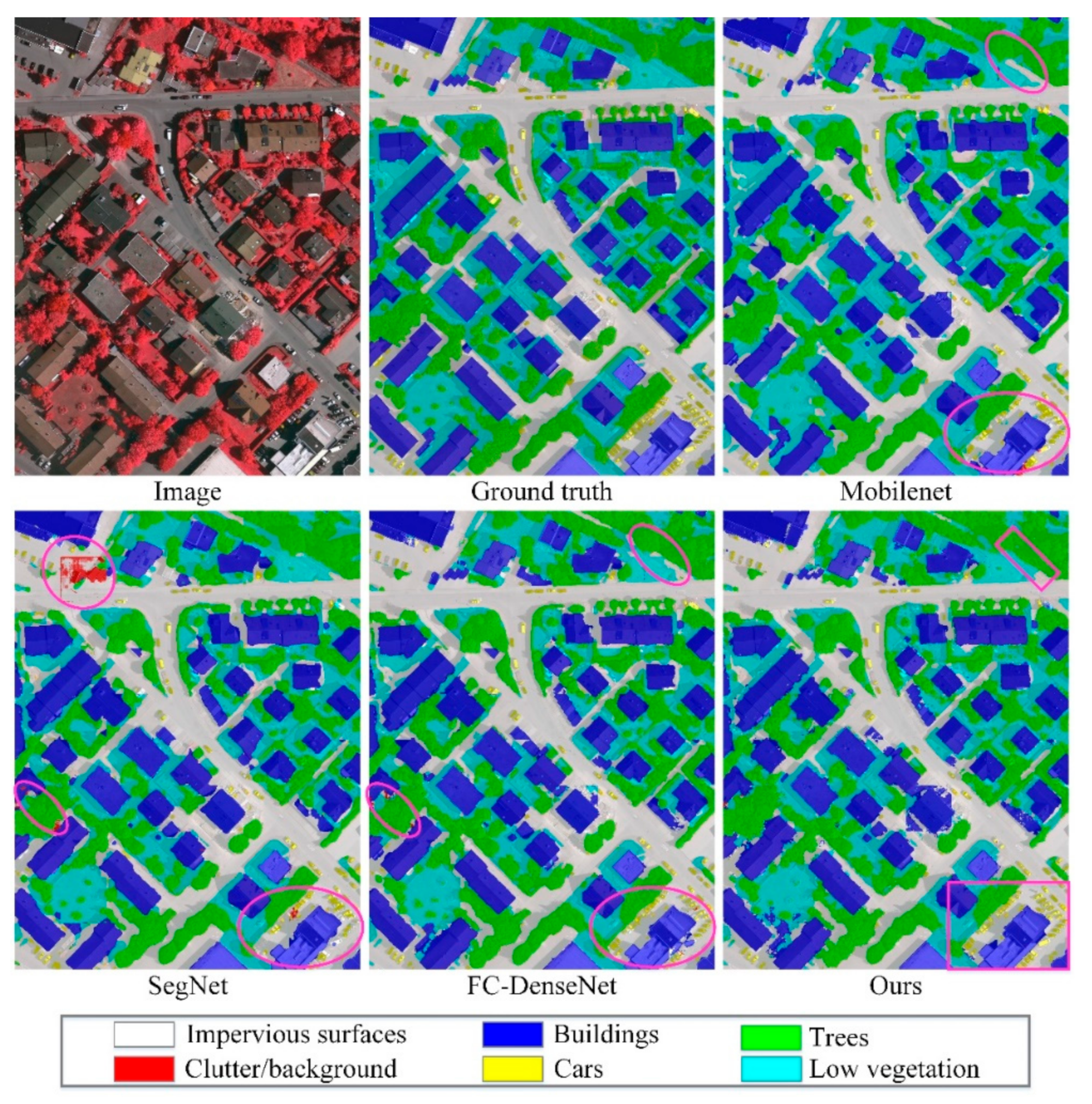
4.3.1. Results of Vaihingen

Table 1 shows the classification results in terms of the per-class accuracy, the mean F1 score, the mIoU, and the overall accuracy (OA) of experiments on the Vaihingen dataset. As a comparison, we also show the results recently published by SVL-boosting + CRF [54], RF + dCRF [55], RotEqNet [56], HSNet [19], and ENR [34] with a model of the same architecture and size as ours. It is demonstrated that REMSNet outperforms other methods in terms of the mean F1 score, mIoU, and overall accuracy. Specifically, comparisons with SegNet, REMSNet obtains increments of 10.33% and 3.04% in mIoU and OA, respectively. This validates the effectiveness of the relation-enhanced blocks and multiscale fusion module in our network. On the whole, the classification performance of different models is very similar, because most methods are in fact variants of FCN or SegNet. Therefore, per-class accuracy is computed to estimate the performance of recognizing distinct objects. The results indicate that our network has a better ability to distinguish objects with similar appearance, such as impervious surfaces and buildings, low vegetation, and trees, because relation-enhanced blocks capture global context relationships to strengthen feature representation. Furthermore, the proposed network achieves high performance in identifying small-scale objects, such as cars. This demonstrates that the multiscale strategy in this paper is effective.
Figure 7 shows examples of classification results on the Vaihingen dataset. Most ground objects are similar in color, such as trees and low vegetation. Moreover, the shadows of trees and buildings also make classification difficult, as shown in Figure 7a,b,e. FC-DenseNet, MobileNet, and SegNet fail to recognize them correctly. The main reason for misclassification is that the networks do not extract useful context information. The proposed method achieves high performance for those classes, which illustrates the effectiveness of the enhanced relation blocks. The classification accuracy of small-scale objects is relatively low, as illustrated in Figure 7c,d. FC-DenseNet, MobileNet, and SegNet cannot segment cars boundary well, while the proposed method can accurately distinguish the cars, because our network captures different-scale ground objects effectively.
To further show the classification performance of our network, Figure 8 shows a full image land cover classification result on the Vaihingen dataset. Figure 8 is generated by overlapping the original aerial image with the land cover classification results, with 60% transparency. In general, our network produces more accurate land cover classification results. In particular, when addressing some easily confused pixels such as trees and low vegetation, and buildings and cars, the proposed method shows better performance.

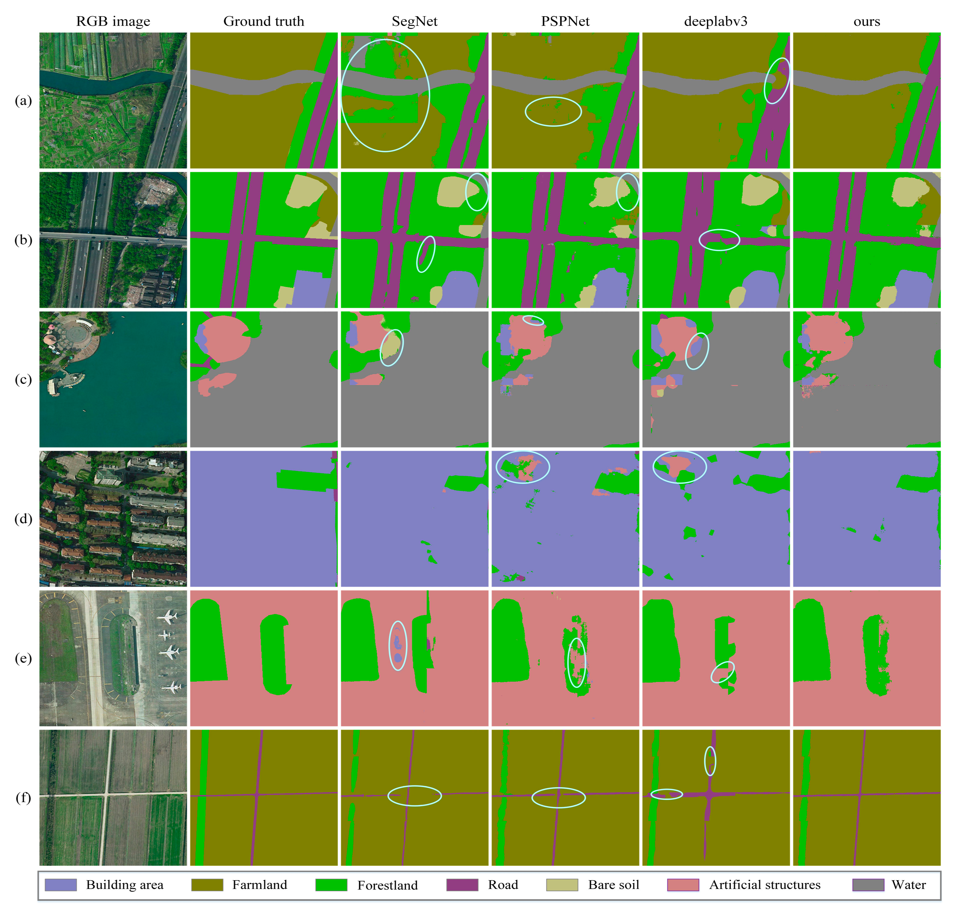
4.3.2. Results of Shanghai

In this subsection, we present the experiments on the Shanghai dataset to further assess the effectiveness of our network. Table 2 shows the quantitative classification results of the Shanghai dataset. As expected, the proposed method outperforms the other approaches in almost every evaluation index. In detail, the method achieved the largest mIoU of up to 73.94%, obtaining an improvement of 6.39% in mIoU compared with FC-DenseNet. The class road of the Shanghai dataset is hard to correctly label in most previous methods because of the shelter of trees and buildings, and the proposed network can achieve an above 8.93% increased accuracy of this class compared to Deeplabv3 because our network captures global context information and fuses different scales ground objects better. Note that the classification accuracy of the artificial structures is generally low due to the relatively small sample size and diversified components.
Figure 9 shows the land cover classification results of our method for the Shanghai aerial image labeling dataset. Figure 9a,b shows that most methods fail to segment the boundaries of farmland and forestland, because they have a similar texture. With the help of enhanced relation blocks, the proposed method achieves better performance when dealing with the same situation. High-resolution aerial images generally have characteristics of high intraclass variance, such as trees in building areas and clutter in artificial structures, as shown in Figure 9c,d,e. The common methods misclassify these classes owing to the lack of global context information. Enhanced relation blocks have a better ability to collect context relationships, reducing the chance of misclassification. Moreover, small-scale ground objects tend to be confused by the networks, as shown in Figure 9f, and roads are divided into discrete sections by most methods, while the proposed method can provide a relatively continuous road segmentation result.
Figure 10 shows a large-scale aerial scene (area S2-1, S2-2, S2-3) as well as urban land cover classification results. The spatial distribution of the different land cover classes can be inferred from these land cover classification results, which can better understand and analyze cities.

5. Discussion

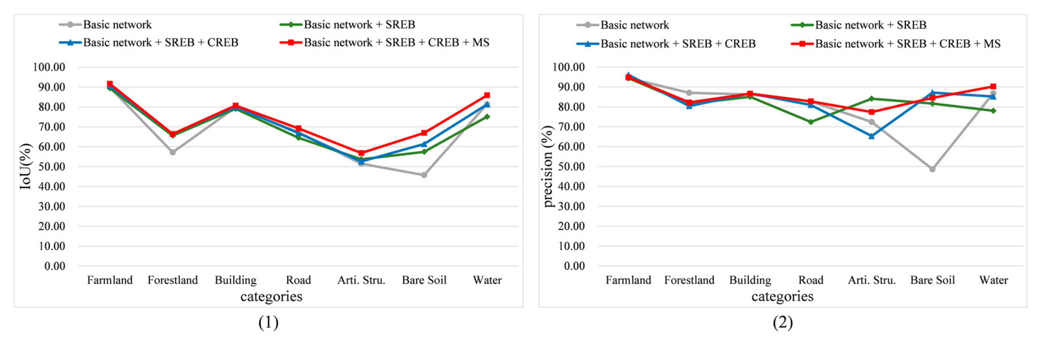
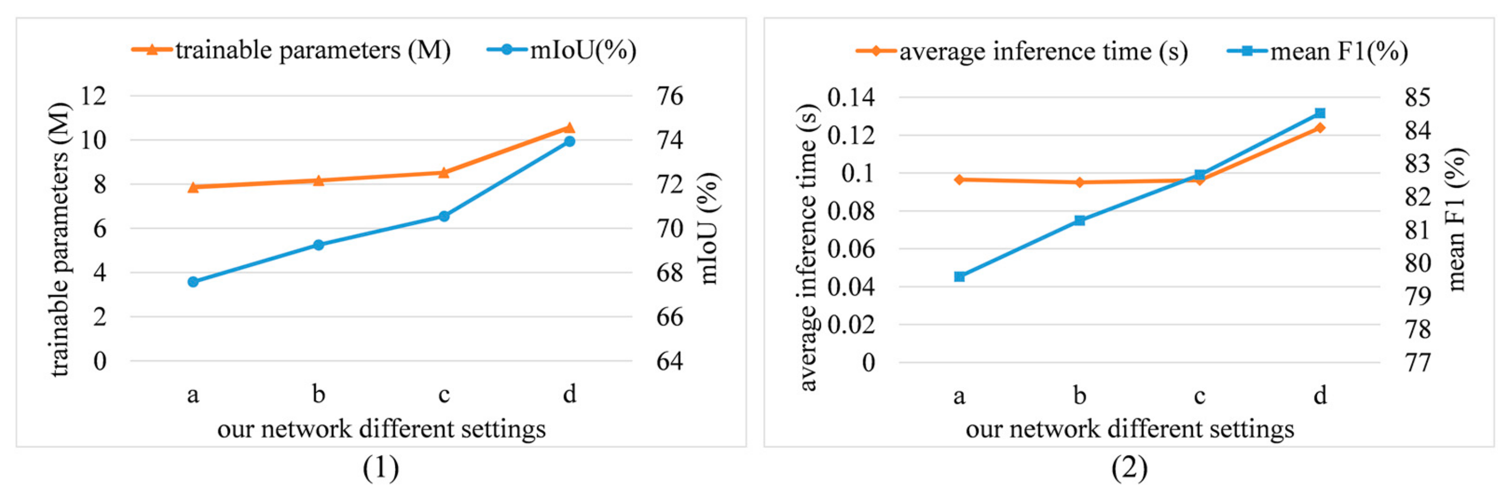
5.1. Influence of the Different Modules on Classification

In our network, spatial and channel relation blocks were employed to explore global context relationships in both spatial and channel domains. Meanwhile, we also designed parallel multi-kernel modules to fuse different-scale features. To evaluate the performance of these modules, we performed experiments with different settings, as shown in Table 3. The ablation experiments were conducted on the Shanghai dataset, where A FC-DenseNet-98 is the basic network. As can be shown in Table 3, relation-enhanced blocks bring a significant improvement as compared to the baseline network. In detail, the mean F 1 and mIoU improved by 4.92% and 6.39% because relation-enhanced blocks help with enhancing useful features while suppressing interference information, improving the segmentation performance. Meanwhile, the multiscale module also improves the performance. The mIoU was improved by 2.63%. The results indicate that multiscale fusion can capture different--scale objects. To further demonstrate the classification performance of different modules, the IoU and precision changes of per class were counted, as shown in Figure 11. In general, relation-enhanced blocks and the multiscale module improve land cover classification results, especially in the category of water and bare soil.
As shown in Figure 12, the classification mIoU and mean F 1 of REMSNet increase with the gradual increase of the different modules, while the number of trainable parameters and the average inference time of the single image did not increase significantly. Trainable parameters increase by 0.66 million and the average inference time is basically unchanged when the network adds relation-enhanced blocks. It is worthy of note that multiscale fusion module increases a greater number of trainable parameters and the inference time compared with other modules. The main reason for this is that parallel multi-kernel deconvolutions in the multiscale fusion module have multiple branches which increases the number of parameters and the inference time.

5.2. Model Size and Efficiency Analysis

In order to analyze the model size and efficiency, we counted the number of trainable parameters and the average inference time of the single image based on the Shanghai dataset. Meanwhile, the accuracy of different models was also counted based on the Shanghai dataset and Vaihingen dataset, as shown in Table 4. All network input image sizes are 256 × 256 pixels. The MobileNet and the proposed REMSNet have fewer trainable parameters. Specifically, the number of trainable parameters of REMSNet reduced by 81% compared with PSPNet. Meanwhile, the REMSNet has the highest mIoU. The results demonstrate the practical utility of the proposed models, especially in the case of limited samples. Our network has a higher-than-average inference time for a single image because the network adopts parallel multi-kernel deconvolutions in the multiscale fusion module. On the one hand, this structure promotes different-level feature fusion; on the other hand, it has multiple branches, which increases the inference time. Our future work will focus on further improving the network computational efficiency in the case of small-sample classification.

6. Conclusions

This study presents a new REMSNet method for urban land cover classification from high-resolution aerial images. The proposed network connectivity pattern is based on DenseNet, which remarkably reduces the number of parameters while maintaining good performance. Meanwhile, the inception module is adopted in the initial encoding stage to overcome the problem of fixed receptive fields. Then, spatial and channel relation-enhanced blocks are used to capture global context information in the spatial and channel domains, respectively, to enhance feature representation and reduce intraclass inconsistency. Finally, the parallel multi-kernel deconvolution module and spatial path in the decoding stage are designed to further aggregate features simultaneously at several scales. The comprehensive ablation studies on the Shanghai dataset show the effectiveness of the proposed modules. In addition, the experimental results based on Vanhigen and Shanghai datasets demonstrate that the proposed REMSNet can obtain comparable or even better performance compared with the state-of-the-art methods while being relatively smaller in terms of the number of trainable parameters. Note that the proposed network computational efficiency is relatively low. In future work, we will focus on further optimizing the network structure and reducing the model size to improve the network computational efficiency.

Author Contributions

Conceptualization and methodology, C.L., D.Z.; Software, D.Z., Y.W.; Validation, D.Z., H.W. and S.J.; Writing—Original draft preparation, D.Z. and C.L.; Writing—Review and editing, C.L., D.Z. and H.W.; Visualization, Y.W. and L.X.; Supervision, H.W. and Y.W.; Funding acquisition, C.L. All authors have read and agreed to the published version of the manuscript.

Funding

This work was supported by the National Key Research and Development Program of China (Grant No.2016YFB0502102 and 2018YFB1305003), and the National Natural Science Foundations of China (Grant No.41771481).

Acknowledgments

The authors thank the anonymous reviewers for their constructive suggestions. The authors thank the Shanghai Surveying and Mapping Institute for providing the Shanghai dataset used in this study. We are also grateful to Akram Akbar, Shuhang Zhang, Wen Zhang, and Jin Zhao for their advice and support in experimental design.

Conflicts of Interest

The authors declare no conflict of interest.

References

  1. Patino, J.E.; Duque, J.C. A review of regional science applications of satellite remote sensing in urban settings. Comput. Environ. Urban Syst. 2013, 37, 1–17. [Google Scholar] [CrossRef]
  2. Qiu, C.; Mou, L.; Schmitt, M.; Zhu, X.X. Local climate zone-based urban land cover classification from multi-seasonal Sentinel-2 images with a recurrent residual network. ISPRS J. Photogramm. Remote Sens. 2019, 154, 151–162. [Google Scholar] [CrossRef] [PubMed]
  3. Yuan, F.; Sawaya, K.E.; Loeffelholz, B.C.; Bauer, M.E. Land cover classification and change analysis of the Twin Cities (Minnesota) Metropolitan Area by multitemporal Landsat remote sensing. Remote Sens. Environ. 2005, 98, 317–328. [Google Scholar] [CrossRef]
  4. Zhu, X.X.; Tuia, D.; Mou, L.; Xia, G.; Zhang, L.; Xu, F.; Fraundorfer, F. Deep Learning in Remote Sensing: A Comprehensive Review and List of Resources. IEEE Geosci. Remote Sens. Mag. 2017, 5, 8–36. [Google Scholar] [CrossRef] [Green Version]
  5. Huang, B.; Zhao, B.; Song, Y.M. Urban land-use mapping using a deep convolutional neural network with high spatial resolution multispectral remote sensing imagery. Remote Sens. Environ. 2018, 214, 73–86. [Google Scholar] [CrossRef]
  6. Belward, A.S.; Skøien, J.O. Who launched what, when and why; trends in global land-cover observation capacity from civilian earth observation satellites. ISPRS J. Photogramm. Remote Sens. 2015, 103, 115–128. [Google Scholar] [CrossRef]
  7. Pesaresi, M.; Huadong, G.; Blaes, X.; Ehrlich, D.; Ferri, S.; Gueguen, L.; Halkia, M.; Kauffmann, M.; Kemper, T.; Lu, L.; et al. A Global Human Settlement Layer from Optical HR/VHR RS Data: Concept and First Results. IEEE J. Sel. Top. Appl. Earth Obs. Remote Sens. 2013, 6, 2102–2131. [Google Scholar] [CrossRef]
  8. Cheng, G.; Zhu, F.; Xiang, S.; Wang, Y.; Pan, C. Accurate urban road centerline extraction from VHR imagery via multiscale segmentation and tensor voting. Neurocomputing 2016, 205, 407–420. [Google Scholar] [CrossRef] [Green Version]
  9. Yuan, Y.; Lin, J.; Wang, Q. Dual-Clustering-Based Hyperspectral Band Selection by Contextual Analysis. IEEE Trans. Geosci. Remote Sens. 2016, 54, 1431–1445. [Google Scholar] [CrossRef]
  10. Sherrah, J. Fully Convolutional Networks for Dense Semantic Labelling of High-Resolution Aerial Imagery. arXiv 2016, arXiv:1606.02585. [Google Scholar]
  11. Zhao, W.; Du, S.; Wang, Q.; Emery, W.J. Contextually guided very-high-resolution imagery classification with semantic segments. ISPRS J. Photogramm. Remote Sens. 2017, 132, 48–60. [Google Scholar] [CrossRef]
  12. Deng, Z.P.; Sun, H.; Zhou, S.L.; Zhao, J.P.; Lei, L.; Zou, H.X. Multi-scale object detection in remote sensing imagery with convolutional neural networks. ISPRS J. Photogramm. Remote Sens. 2018, 145, 3–22. [Google Scholar] [CrossRef]
  13. Long, J.; Shelhamer, E.; Darrell, T. Fully convolutional networks for semantic segmentation. In Proceedings of the 2015 IEEE Conference on Computer Vision and Pattern Recognition (CVPR), Piscataway, NJ, USA, 7–12 June 2015; pp. 3431–3440. [Google Scholar]
  14. Yu, B.; Yang, L.; Chen, F. Semantic Segmentation for High Spatial Resolution Remote Sensing Images Based on Convolution Neural Network and Pyramid Pooling Module. IEEE J. Sel. Top. Appl. Earth Obs. Remote Sens. 2018, 11, 3252–3261. [Google Scholar] [CrossRef]
  15. Chen, L.-C.; Papandreou, G.; Schroff, F.; Adam, H. Rethinking Atrous Convolution for Semantic Image Segmentation. arXiv 2017, arXiv:1706.05587. [Google Scholar]
  16. Zhang, P.; Ke, Y.; Zhang, Z.; Wang, M.; Li, P.; Zhang, S. Urban Land Use and Land Cover Classification Using Novel Deep Learning Models Based on High Spatial Resolution Satellite Imagery. Sensors 2018, 18, 3717. [Google Scholar] [CrossRef] [PubMed] [Green Version]
  17. Panboonyuen, T.; Jitkajornwanich, K.; Lawawirojwong, S.; Srestasathiern, P.; Vateekul, P. Semantic Segmentation on Remotely Sensed Images Using an Enhanced Global Convolutional Network with Channel Attention and Domain Specific Transfer Learning. Remote Sens. 2019, 11, 83. [Google Scholar] [CrossRef] [Green Version]
  18. Peng, C.; Zhang, X.; Yu, G.; Luo, G.; Sun, J. Large Kernel Matters—Improve Semantic Segmentation by Global Convolutional Network. In Proceedings of the 2017 IEEE Conference on Computer Vision and Pattern Recognition (CVPR), Honolulu, HI, USA, 21–26 July 2017; pp. 1743–1751. [Google Scholar]
  19. Liu, Y.; Minh Nguyen, D.; Deligiannis, N.; Ding, W.; Munteanu, A. Hourglass-ShapeNetwork Based Semantic Segmentation for High Resolution Aerial Imagery. Remote Sens. 2017, 9, 522. [Google Scholar] [CrossRef] [Green Version]
  20. Chen, G.; Zhang, X.; Wang, Q.; Dai, F.; Gong, Y.; Zhu, K. Symmetrical Dense-Shortcut Deep Fully Convolutional Networks for Semantic Segmentation of Very-High-Resolution Remote Sensing Images. IEEE J. Sel. Top. Appl. Earth Obs. Remote Sens. 2018, 11, 1633–1644. [Google Scholar] [CrossRef]
  21. Ronneberger, O.; Fischer, P.; Brox, T. U-Net: Convolutional networks for biomedical image segmentation. In Proceedings of the 2015 Medical Image Computing and Computer-Assisted Intervention (MICCAI), Cham, Switzerland, 5–9 October 2015; pp. 234–241. [Google Scholar]
  22. Wang, Q.; Liu, S.; Chanussot, J.; Li, X. Scene Classification with Recurrent Attention of VHR Remote Sensing Images. IEEE Trans. Geosci. Remote Sens. 2019, 57, 1155–1167. [Google Scholar] [CrossRef]
  23. Mou, L.; Ghamisi, P.; Zhu, X.X. Deep Recurrent Neural Networks for Hyperspectral Image Classification. IEEE Trans. Geosci. Remote Sens. 2017, 55, 3639–3655. [Google Scholar] [CrossRef] [Green Version]
  24. Xiaolong, W.; Girshick, R.; Gupta, A.; Kaiming, H. Non-local neural networks. In Proceedings of the 2018 IEEE/CVF Conference on Computer Vision and Pattern Recognition, Los Alamitos, CA, USA, 18–23 June 2018; pp. 7794–7803. [Google Scholar]
  25. Huang, G.; Liu, Z.; Maaten, L.v.d.; Weinberger, K.Q. Densely Connected Convolutional Networks. In Proceedings of the 2017 IEEE Conference on Computer Vision and Pattern Recognition (CVPR), Honolulu, HI, USA, 21–26 July 2017; pp. 2261–2269. [Google Scholar]
  26. Szegedy, C.; Wei, L.; Yangqing, J.; Sermanet, P.; Reed, S.; Anguelov, D.; Erhan, D.; Vanhoucke, V.; Rabinovich, A. Going deeper with convolutions. In Proceedings of the 2015 IEEE Conference on Computer Vision and Pattern Recognition (CVPR), Boston, MA, USA, 7–12 June 2015; pp. 1–9. [Google Scholar]
  27. Garcia-Garcia, A.; Orts-Escolano, S.; Oprea, S.; Villena-Martinez, V.; Martinez-Gonzalez, P.; Garcia-Rodriguez, J. A survey on deep learning techniques for image and video semantic segmentation. Appl. Soft Comput. 2018, 70, 41–65. [Google Scholar] [CrossRef]
  28. Ma, L.; Liu, Y.; Zhang, X.; Ye, Y.; Yin, G.; Johnson, B.A. Deep learning in remote sensing applications: A meta-analysis and review. ISPRS J. Photogramm. Remote Sens. 2019, 152, 166–177. [Google Scholar] [CrossRef]
  29. Sun, W.W.; Wang, R.S. Fully Convolutional Networks for Semantic Segmentation of Very High Resolution Remotely Sensed Images Combined With DSM. IEEE Geosci. Remote Sens. Lett. 2018, 15, 474–478. [Google Scholar] [CrossRef]
  30. Zhao, H.; Shi, J.; Qi, X.; Wang, X.; Jia, J. Pyramid Scene Parsing Network. In Proceedings of the 2017 IEEE Conference on Computer Vision and Pattern Recognition (CVPR), Honolulu, HI, USA, 21–26 July 2017; pp. 6230–6239. [Google Scholar]
  31. Badrinarayanan, V.; Kendall, A.; Cipolla, R. SegNet: A Deep Convolutional Encoder-Decoder Architecture for Image Segmentation. IEEE Trans. Pattern Anal. Mach. Intell. 2017, 39, 2481–2495. [Google Scholar] [CrossRef] [PubMed]
  32. Sun, T.; Chen, Z.; Yang, W.; Wang, Y. Stacked U-Nets with Multi-output for Road Extraction. In Proceedings of the 2018 IEEE/CVF Conference on Computer Vision and Pattern Recognition Workshops (CVPRW), Salt Lake City, UT, USA, 18–22 June 2018; pp. 187–1874. [Google Scholar]
  33. Marmanis, D.; Schindler, K.; Wegner, J.D.; Galliani, S.; Datcu, M.; Stilla, U. Classification with an edge: Improving semantic image segmentation with boundary detection. ISPRS J. Photogramm. Remote Sens. 2018, 135, 158–172. [Google Scholar] [CrossRef] [Green Version]
  34. Liu, S.; Ding, W.; Liu, C.; Liu, Y.; Wang, Y.; Li, H. ERN: Edge Loss Reinforced Semantic Segmentation Network for Remote Sensing Images. Remote Sens. 2018, 10, 1339. [Google Scholar] [CrossRef] [Green Version]
  35. Audebert, N.; Le Saux, B.; Lefèvre, S. Beyond RGB: Very high resolution urban remote sensing with multimodal deep networks. ISPRS J. Photogramm. Remote Sens. 2018, 140, 20–32. [Google Scholar] [CrossRef] [Green Version]
  36. He, K.; Zhang, X.; Ren, S.; Sun, J. Deep Residual Learning for Image Recognition. In Proceedings of the 2016 IEEE Conference on Computer Vision and Pattern Recognition (CVPR), Las Vegas, NV, USA, 27–30 June 2016; pp. 770–778. [Google Scholar]
  37. Sun, Y.; Zhang, X.; Xin, Q.; Huang, J. Developing a multi-filter convolutional neural network for semantic segmentation using high-resolution aerial imagery and LiDAR data. ISPRS J. Photogramm. Remote Sens. 2018, 143, 3–14. [Google Scholar] [CrossRef]
  38. Feng, W.; Sui, H.; Huang, W.; Xu, C.; An, K. Water Body Extraction from Very High-Resolution Remote Sensing Imagery Using Deep U-Net and a Superpixel-Based Conditional Random Field Model. IEEE Geosci. Remote Sens. Lett. 2019, 16, 618–622. [Google Scholar] [CrossRef]
  39. Krähenbühl, P.; Science, V.K.J.C. Efficient Inference in Fully Connected CRFs with Gaussian Edge Potentials. In Proceedings of the 2011 Neural Information Processing Systems (NIPS), Granada, Spain, 12–15 December 2011; pp. 109–117. [Google Scholar]
  40. Zheng, S.; Jayasumana, S.; Romera-Paredes, B.; Vineet, V.; Su, Z.; Du, D.; Huang, C.; Torr, P.H.S. Conditional Random Fields as Recurrent Neural Networks. In Proceedings of the 2015 IEEE International Conference on Computer Vision (ICCV), Santiago, Chile, 13–16 December 2015; pp. 1529–1537. [Google Scholar]
  41. He, C.; Fang, P.; Zhang, Z.; Xiong, D.; Liao, M. An End-to-End Conditional Random Fields and Skip-Connected Generative Adversarial Segmentation Network for Remote Sensing Images. Remote Sens. 2019, 11, 1604. [Google Scholar] [CrossRef] [Green Version]
  42. Bahdanau, D.; Cho, K.; Bengio, Y. Neural machine translation by jointly learning to align and translate. In Proceedings of the 2015 International Conference on Learning Representations (ICLR), San Diego, CA, USA, 7–9 May 2015. [Google Scholar]
  43. Li, H.; Xiong, P.; An, J.; Wang, L. Pyramid attention network for semantic segmentation. In Proceedings of the 2018 British Machine Vision Conference (BMVC), Newcastle, UK, 3–6 September 2018. [Google Scholar]
  44. Vaswani, A.; Shazeer, N.; Parmar, N.; Uszkoreit, J.; Jones, L.; Gomez, A.N.; Kaiser, L.; Polosukhin, I. Attention is all you need. In Proceedings of the 31st Annual Conference on Neural Information Processing Systems (NIPS), Long Beach, CA, USA, 4–9 December 2017; pp. 5999–6009. [Google Scholar]
  45. Zhao, H.; Zhang, Y.; Liu, S.; Shi, J.; Loy, C.C.; Lin, D.; Jia, J. PSANet: Point-wise Spatial Attention Network for Scene Parsing. In Proceedings of the 2018 European Conference on Computer Vision (ECCV), Cham, Switzerland, 8–14 September 2018; pp. 270–286. [Google Scholar]
  46. Yuan, Y.; Wang, J. OCNet: Object Context Network for Scene Parsing. arXiv 2018, arXiv:1809.00916. [Google Scholar]
  47. Chen, L.-C.; Yang, Y.; Wang, J.; Xu, W.; Yuille, A.L. Attention to Scale: Scale-Aware Semantic Image Segmentation. In Proceedings of the 29th IEEE Conference on Computer Vision and Pattern Recognition (CVPR), Las Vegas, NV, USA, 1–26 June 2016; pp. 3640–3649. [Google Scholar]
  48. Jie, H.; Li, S.; Gang, S. Squeeze-and-excitation Networks. In Proceedings of the 2018 IEEE/CVF Conference on Computer Vision and Pattern Recognition, Los Alamitos, CA, USA, 18–23 June 2018; pp. 7132–7141. [Google Scholar]
  49. Woo, S.; Park, J.; Lee, J.-Y.; Kweon, I.S. CBAM: Convolutional Block Attention Module. In Proceedings of the 2018 European Conference on Computer Vision (ECCV), Cham, Switzerland, 8–14 September 2018; pp. 3–19. [Google Scholar]
  50. Jégou, S.; Drozdzal, M.; Vazquez, D.; Romero, A.; Bengio, Y. The One Hundred Layers Tiramisu: Fully Convolutional DenseNets for Semantic Segmentation. In Proceedings of the IEEE Computer Society Conference, Honolulu, HI, USA, 21–26 July 2017; pp. 1175–1183. [Google Scholar]
  51. Huang, Z.; Wang, X.; Huang, L.; Huang, C.; Wei, Y.; Liu, W. CCNet: Criss-Cross Attention for Semantic Segmentation. arXiv 2018, arXiv:1811.11721. [Google Scholar]
  52. Yu, C.; Wang, J.; Peng, C.; Gao, C.; Yu, G.; Sang, N. BiSeNet: Bilateral segmentation network for real-time semantic segmentation. In Proceedings of the 15th European Conference on Computer Vision (ECCV), Munich, Germany, 8–14 September 2018; pp. 334–349. [Google Scholar]
  53. 2D Semantic Labeling—Vaihingen Data. Available online: http://www2.isprs.org/commissions/comm3/wg4/2d-sem-label-vaihingen.html (accessed on 5 November 2019).
  54. Gerke, M. Use of the Stair Vision Library within the ISPRS 2D Semantic Labeling Benchmark (Vaihingen); Technical Report; University of Twente: Enschede, The Netherlands, 2015. [Google Scholar]
  55. Quang, N.T.; Sang, D.V.; Thuy, N.T.; Binh, H.T.T. An efficient framework for pixel-wise building segmentation from aerial images. In Proceedings of the 6th International Symposium on Information and Communication Technology (SoICT), Hue, Vietnam, 3–4 December 2015; pp. 282–287. [Google Scholar]
  56. Marcos, D.; Volpi, M.; Kellenberger, B.; Tuia, D. Land cover mapping at very high resolution with rotation equivariant CNNs: Towards small yet accurate models. ISPRS J. Photogramm. Remote Sens. 2018, 145, 96–107. [Google Scholar] [CrossRef] [Green Version]
  57. Abadi, M.; Barham, P.; Chen, J.; Chen, Z.; Davis, A.; Dean, J.; Devin, M.; Ghemawat, S.; Irving, G.; Isard, M.; et al. TensorFlow: A system for large-scale machine learning. In Proceedings of the 12th USENIX conference on Operating Systems Design and Implementation, Savannah, GA, USA, 2–4 November 2016; pp. 265–283. [Google Scholar]
  58. Hinton, G.; Tieleman, T. Lecture 6.5-Rmsprop, Coursera: Neural Networks for Machine Learning; Technical Report; University of Toronto: Toronto, ON, Canada, 2012. [Google Scholar]
  59. Howard, A.G.; Zhu, M.; Chen, B.; Kalenichenko, D.; Wang, W.; Weyand, T.; Andreetto, M.; Adam, H. MobileNets: Efficient Convolutional Neural Networks for Mobile Vision Applications. arXiv 2017, arXiv:1704.04861. [Google Scholar]
Figure 1. Relation-enhanced multiscale convolutional network (REMSNet) overview.
Remotesensing 12 00311 g001
Figure 2. Different blocks neural network units. (a) Inception block; (b) dense block (layer = 3, k = 3); (c) residual block [36].
Remotesensing 12 00311 g002
Figure 3. The basic principle chart of relation-enhanced blocks. (a) Spatial relation-enhanced block; (b) channel relation-enhanced block.
Remotesensing 12 00311 g003
Figure 4. Examples of Vaihingen dataset. (a) Aerial image; (b) ground truth; (c) ground truth with eroded boundaries (black areas will be ignored); (d) corresponding Normalized Digital Surface Model (nDSM).
Remotesensing 12 00311 g004
Figure 5. Study areas and image data of the Shanghai dataset.
Remotesensing 12 00311 g005
Figure 6. Examples of Shanghai dataset. (a) Aerial image; (b) corresponding ground truth.
Remotesensing 12 00311 g006
Figure 7. Examples of land cover classification results on the Vaihingen dataset. The rectangles in pink and the circles in pink represent correct and incorrect classification, respectively. (ae) are five subsets land cover classification results from Vaihingen dataset.
Remotesensing 12 00311 g007
Figure 8. A full image land cover classification result on the Vaihingen dataset. The circles in pink and the rectangle in pink represent the correct and incorrect classification, respectively.
Remotesensing 12 00311 g008
Figure 9. Examples of land cover classification results for the Shanghai dataset. The circles in white represent incorrect classification. (af) are six subsets land cover classification results from Shanghai dataset.
Remotesensing 12 00311 g009
Figure 10. Urban land cover classification map using the proposed network.
Remotesensing 12 00311 g010
Figure 11. Intersection-over-union (IoU) and precision changes of per class with different settings. (1) Changes of per class IoU with different settings; (2) changes of per class precision with different settings. SREB: spatial relation-enhanced block; CREB: channel relation-enhanced block; MS: multiscale fusion module.
Remotesensing 12 00311 g011
Figure 12. Our network different settings’ speed and accuracy analysis for the Shanghai dataset. (1) Changes of trainable parameters and mIoU with different settings; (2) changes of the average inference time and mean F 1   with different settings; a: Basic network; b: basic network + SREB; c: basic network + SREB + CREB; d: basic network + SREB + CREB + MS.
Remotesensing 12 00311 g012
Table 1. Experimental land cover classification results on the Vaihingen dataset (%). The largest land cover classification accuracy is highlighted in bold.
MethodImp. Surf.BuildingsLow Veg.TreeCar Mean   F 1   mIoUOA
SVL-boosting + CRF [54] 86.1090.9077.6084.9059.9079.90-84.70
RF + dCRF [55] 86.9092.0078.386.9029.0074.60-85.90
SegNet [31]92.2793.7377.3586.6562.7681.2770.4087.42
MobileNet [59]90.2994.1383.1384.0777.1985.5675.5687.76
FC-DenseNet [50]92.4094.4672.9590.9378.4986.7377.2087.99
RotEqNet [56] 89.5094.8077.5086.50 72.6084.18-87.50
HSNet [19] 90.8994.5178.8387.84 81.8786.79-88.32
ENR [34] 91.4895.1179.4288.18 89.0088.64-88.88
REMSNet 92.0795.9583.5390.1381.4889.0780.7390.46
Table 2. Experimental land cover classification results on the Shanghai dataset (%). The largest land cover classification accuracy is highlighted in bold.
MethodFarmlandForestlandBuildingRoadArti. Stru.Bare SoilWater Mean   F 1   mIoUOA
FC-DenseNet [50]94.9262.5291.4978.3863.9988.4592.7479.6067.5585.20
SegNet [31]92.8775.8691.6676.4961.2970.3393.280.1768.0285.68
MobileNet [59]96.0370.4291.5377.6161.1679.2888.1480.5468.5986.18
Deeplabv3 [15]95.2877.2789.3472.9358.6076.7789.8680.9068.9786.19
PSPNet [30]93.6776.0291.4475.7463.4376.2993.0081.7170.0586.36
REMSNet96.2177.5192.5981.8663.9581.8193.5684.5273.9488.55
Table 3. Detailed performance of the proposed network with different settings. SREB: spatial relation-enhanced block; CREB: channel relation-enhanced block; MS: multiscale fusion module. The largest classification accuracy is highlighted in bold.
Method Mean   F 1   ( % ) OA (%)mIoU (%)
Basic network79.6085.2067.55
Basic network + SREB81.2886.7769.25
Basic network + SREB + CREB82.6687.4271.31
Basic network + SREB + CREB + MS84.5288.5573.94
Table 4. Different model size and efficiency analysis. “M” stands for million; “Shang.” Stands Shanghai dataset; “Vaihi.” Stands Vaihingen dataset.
MethodParameters (M)Time (s)Mean F 1 (%)OA (%)mIoU (%)
Shang.Vaihi.Shang.Vaihi.Shang.Vaihi.
FC-DenseNet [50]7.860.096579.6086.7385.2087.9967.5577.20
SegNet [31]34.960.035080.1781.2785.6887.4268.0270.40
MobileNet [59]8.870.032580.5485.5686.1887.7668.5975.56
Deeplabv3 [15] 46.660.013080.90-86.19-68.97-
PSPNet [30]55.990.021781.71-86.36-70.05-
REMSNet10.560.123984.5289.0788.5590.4673.9480.73

