The Determination of Snow Albedo from Satellite Measurements Using Fast Atmospheric Correction Technique

 , , , ,
Abstract
:
1. Introduction
2. Materials and Methods
2.1. Theory
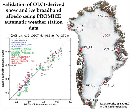
2.2. Validation
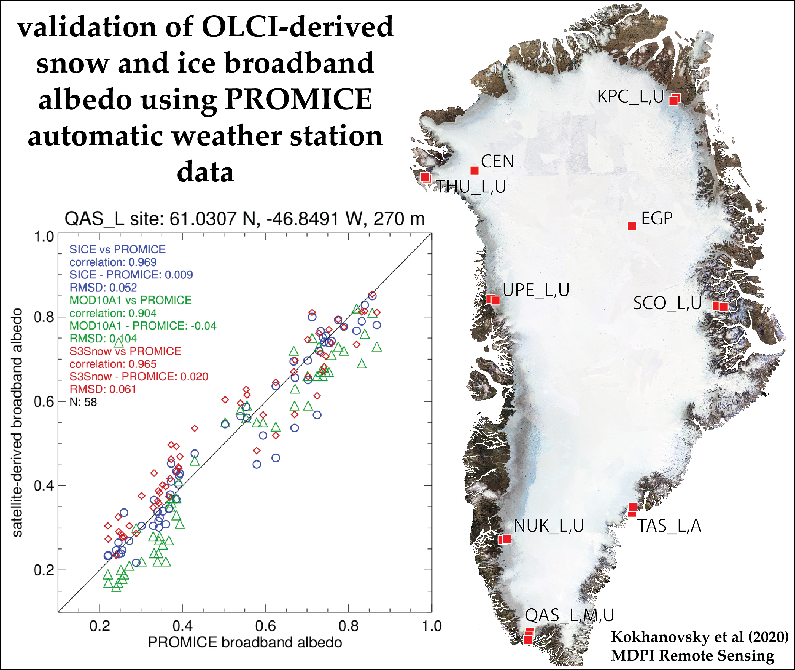
2.2.1. Snow Spectral Albedo
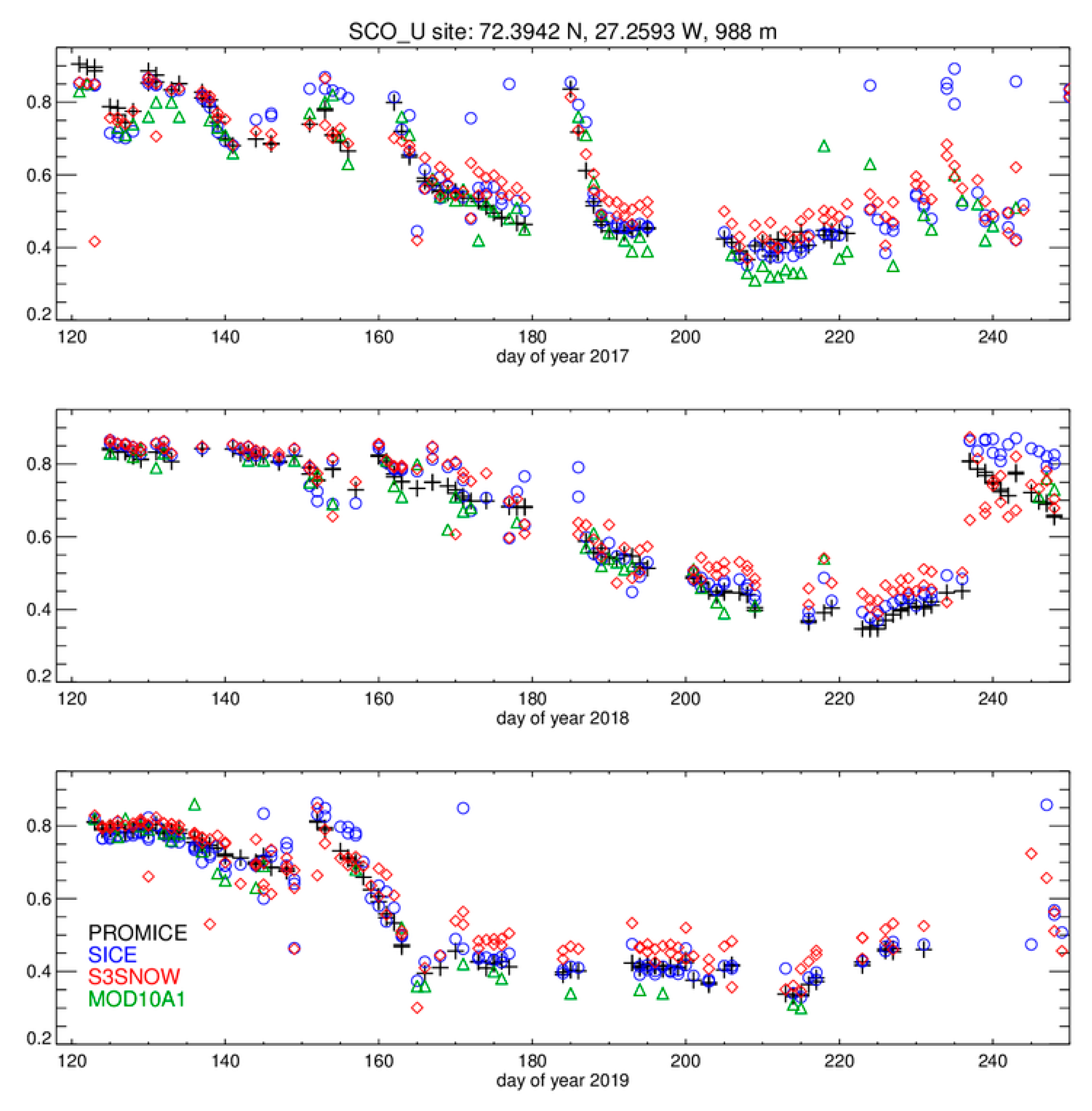
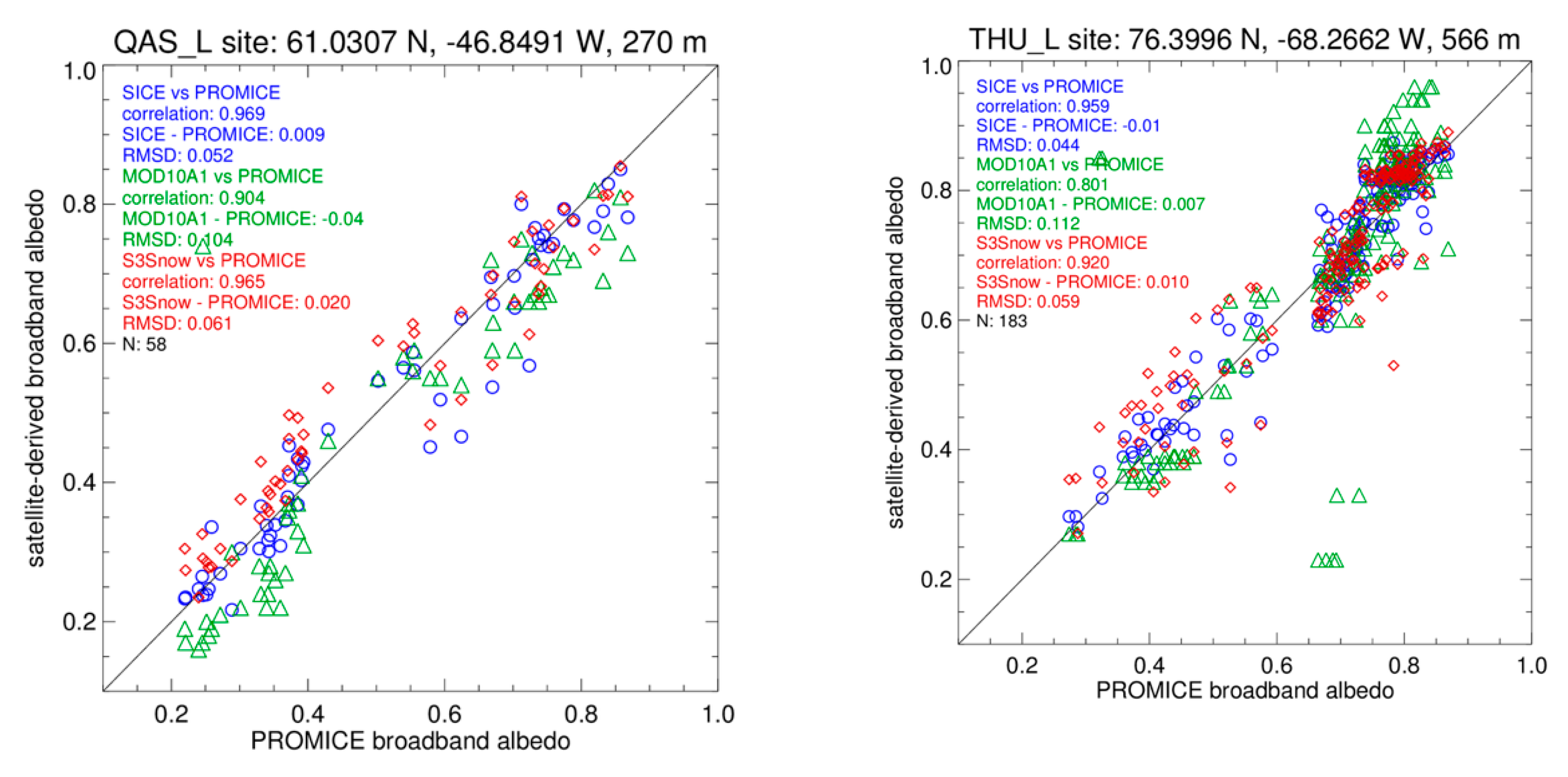
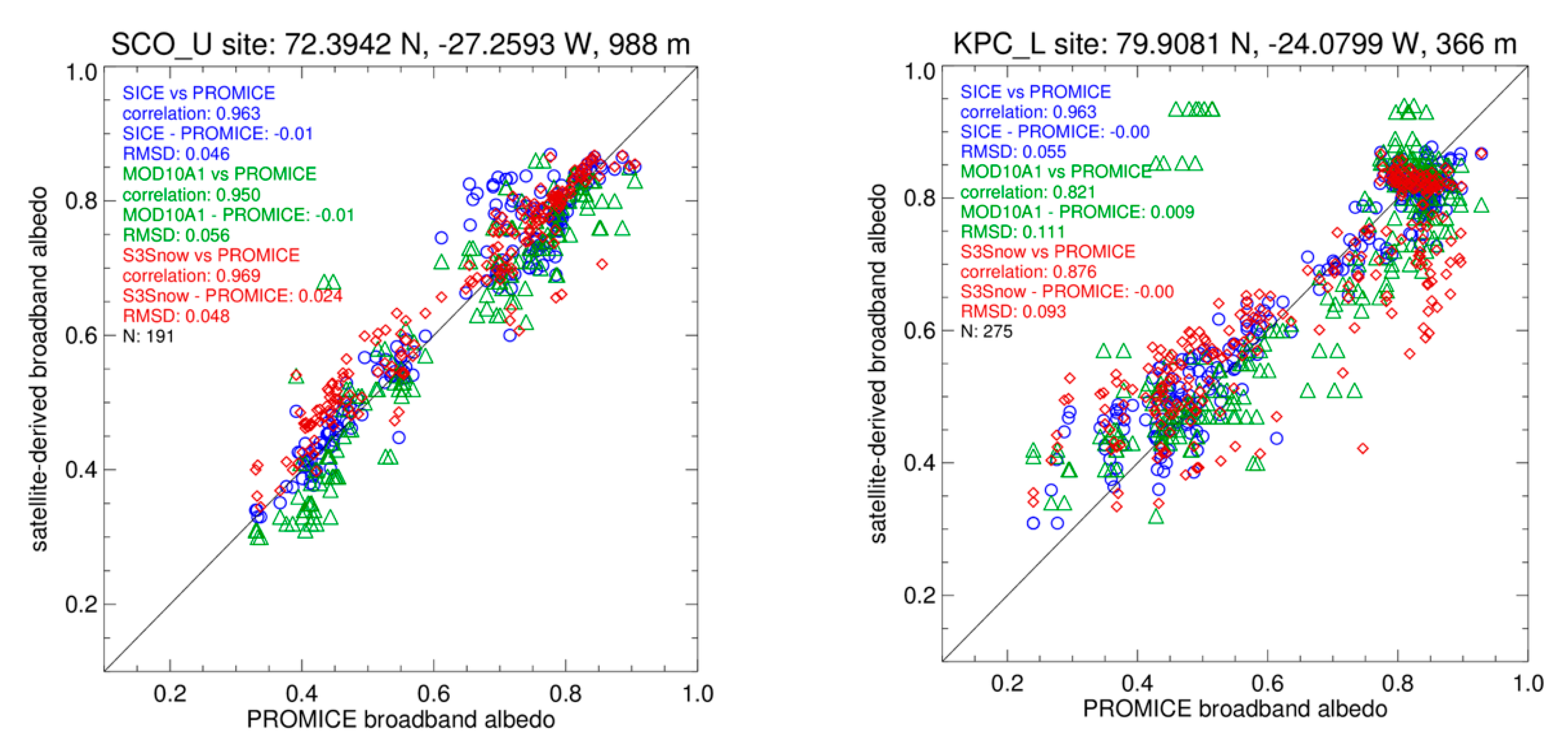
2.2.2. Snow Broadband Albedo
3. Discussion
4. Conclusions
Author Contributions
Funding
Acknowledgments
Conflicts of Interest
Appendix A. Atmospheric Radiative Transfer: Simple Approximations


| , nm | |
|---|---|
| 400.00000 | 1.378170469 × 10⁻⁴ |
| 412.50000 | 3.048780958 × 10⁻⁴ |
| 442.50000 | 1.645714060 × 10⁻³ |
| 490.00000 | 8.935947110 × 10⁻³ |
| 510.00000 | 1.750535146 × 10⁻² |
| 560.00000 | 4.347104369 × 10⁻² |
| 620.00000 | 4.487130794 × 10⁻² |
| 665.00000 | 2.101591797 × 10⁻² |
| 673.75000 | 1.716230955 × 10⁻² |
| 681.25000 | 1.466298300 × 10⁻² |
| 708.75000 | 7.983028470 × 10⁻³ |
| 753.75000 | 3.879744653 × 10⁻³ |
| 761.25000 | 2.923775641 × 10⁻³ |
| 764.37500 | 2.792211429 × 10⁻³ |
| 767.50000 | 2.729651478 × 10⁻³ |
| 778.75000 | 3.255969698 × 10⁻³ |
| 865.00000 | 8.956858078 × 10⁻⁴ |
| 885.00000 | 5.188799343 × 10⁻⁴ |
| 900.00000 | 6.715773241 × 10⁻⁴ |
| 940.00000 | 3.127781417 × 10⁻⁴ |
| 1020.00000 | 1.408798425 × 10⁻⁵ |
References
- Vinnikov, K.Y.; Robock, A.; Stouffer, R.J.; Walsh, J.E.; Parkinson, C.L.; Cavalieri, D.J.; Mitchell, J.F.B.; Garrett, D.; Zakharov, V.F. Global warming and Northern Hemisphere sea ice extent. Science 1999, 286, 1934–1937. [Google Scholar] [CrossRef] [PubMed]
- Hansen, J.; Nazarenko, L. Soot climate forcing via snow and ice albedos. Proc. Natl. Acad. Sci. USA 2004, 101, 423–428. [Google Scholar] [CrossRef] [PubMed] [Green Version]
- Stroeve, J.; Box, J.E.; Wang, Z.; Schaaf, C.; Barrett, A. Re-evaluation of MODIS MCD43 Greenland albedo accuracy and trends. Remote Sens. Environ. 2013, 138, 199–214. [Google Scholar] [CrossRef]
- Kokhanovsky, A.; Tomasi, C. (Eds.) Physics and Chemistry of Arctic Atmosphere; Springer: Berlin, Germany, 2020; in press. [Google Scholar]
- Schaaf, C.B.; Gao, F.; Strahler, A.H.; Lucht, W.; Li, X.; Tsang, T.; Strugnell, N.C.; Zhang, X.; Jin, Y.; Muller, J.-P. First operational BRDF, albedo and nadir reflectance products from MODIS. Remote Sens. Environ. 2002, 83, 135–148. [Google Scholar] [CrossRef] [Green Version]
- Kokhanovsky, A.A.; Lamare, M.; Danne, O.; Dumont, M.; Brockmann, C.; Picard, G.; Arnaud, L.; Favier, V.; Jourdain, B.; Lemeur, E.; et al. Retrieval of Snow Properties from the Sentinel-3 Ocean and Land Colour Instrument. Remote Sens. 2019, 11, 2280. [Google Scholar] [CrossRef] [Green Version]
- Dang, C.; Brandt, R.E.; Warren, S.G. Parameterizations for narrowband and broadband albedo of pure snow, and snow containing mineral dust and black carbon. J. Geophys. Res. 2015, 120. [Google Scholar] [CrossRef]
- Morel, A.; Prieur, L. Analysis of variations in ocean color. Limnol. Oceanogr. 1977, 22, 709–722. [Google Scholar] [CrossRef]
- Mobley, C.D.; Stramski, D.; Bissett, W.P.; Boss, E. Optical modeling of ocean waters: Is the Case 1–Case 2 classification still useful? Oceanography 2004, 17, 60–67. [Google Scholar] [CrossRef]
- Liou, K.-N. An Introduction to Atmospheric Radiation; Academic Press: New York, NY, USA, 2002. [Google Scholar]
- Kokhanovsky, A.; Mayer, B.; Rozanov, V.V. A parameterization of the diffuse transmittance and reflectance for aerosol remote sensing problems. Atmos. Res. 2005, 73, 37–43. [Google Scholar] [CrossRef] [Green Version]
- Ricchiazzi, P.; Yang, S.; Gautier, C.; Sowle, D. SBDART, A research and teaching tool for plane-parellel radiative transfer in the Earth’s atmosphere. Bull. Am. Meteorol. Soc. 1998, 79, 2101–2114. [Google Scholar] [CrossRef] [Green Version]
- Shettle, E.P.; Fenn, R.W. Models for the Aerosols of the Lower Atmosphere and the Effects of Humidity Variations on Their Properties; Report AFGt-TR-79-O21 1979; Air Force Geophysical Laboratory: Middlesex County, MA, USA, 1979. [Google Scholar]
- Aoki, T.; Kuchiki, K.; Niwano, M.; Kodama, Y.; Hosaka, M.; Tanaka, T. Physically based snow albedo model for calculating broadband albedos and the solar heating profile in snowpack for general circulation models. J. Geophys. Res. Atmos. 2011, 116, D11114. [Google Scholar] [CrossRef]
- Hall, D.K.; Riggs, G.A. MODIS/Terra Snow Cover Daily L3 Global 500m Grid, Version 6. Greenland Coverage; National Snow and Ice Data Center: Boulder, CO, USA; NASA Distributed Active Archive Center: Boulder, CO, USA, 2016. Available online: http://nsidc.org/data/MOD10A1/versions/6 (accessed on 1 October 2019).
- Sobolev, V.V. Light Scattering in Planetary Atmospheres; Nauka: Moscow, Russia, 1972. [Google Scholar]
- Katsev, I.L.; Prikhach, A.S.; Zege, E.P.; Grudo, J.O.; Kokhanovsky, A.A. Speeding up the aerosol optical thickness retrieval using analytical solutions of radiative transfer theory. Atmos. Meas. Tech. 2010, 3, 1403–1422. [Google Scholar] [CrossRef]
- Leckner, B. The Spectral Distribution of Solar Radiation at the Earth’s Surface-Elements of a Model. Sol. Energy 1978, 20, 143–150. [Google Scholar] [CrossRef]
- Iqbal, M. An Introduction to Solar Radiation; Academic Press: New York, NY, USA, 1983; pp. 114–115. [Google Scholar]
- Kinne, S. The MACv2 Aerosol Climatology. Tellus B 2019, 71, 1–21. [Google Scholar] [CrossRef] [Green Version]
- Holben, B.N.; Tanré, D.; Smirnov, A.; Eck, T.F.; Slutsker, I.; Abuhassan, N.; Newcomb, W.W.; Schafer, J.S.; Chatenet, B.; Lavenu, F.; et al. An emerging ground-based aerosol climatology: Aerosol optical depth from AERONET. J. Geophys. Res. 2001, 106, 12067–12097. [Google Scholar] [CrossRef]
- Giles, D.M.; Sinyuk, A.; Sorokin, M.G.; Schafer, J.S.; Smirnov, A.; Slutsker, I.; Eck, T.F.; Holben, B.N.; Lewis, J.R.; Campbell, J.R.; et al. Advancements in the Aerosol Robotic Network (AERONET) Version 3 database—Automated near real-time quality control algorithm with improved cloud screening for Sun photometer aerosol optical depth (AOD) measurements. Atmos. Meas. Tech. 2019, 12, 169–209. [Google Scholar] [CrossRef] [Green Version]
- Sinyuk, A.; Holben, B.N.; Eck, T.F.; Giles, D.M.; Slutsker, I.; Korkin, S.; Schafer, J.S.; Smirnov, A.; Sorokin, M.; Lyapustin, A. The AERONET Version 3 aerosol retrieval algorithm, associated uncertainties and comparisons to Version 2. Atmos. Meas. Tech. 2020. in review. [Google Scholar] [CrossRef] [Green Version]
- Kokhanovsky, A.A.; Lamare, M.; Rozanov, V.V.; Danne, O. The retrieval of total ozone over snow using Ocean and Land Colour Instrument. J. Quant. Spectrosc. Radiat. Transf. 2020, 11, 2280. [Google Scholar]


| , 1/Microns | , 1/Microns | |||
|---|---|---|---|---|
| 3.238 × 101 | −1.6014033 × 10⁵ | 7.95953 × 10³ | 1.778 × 10³ | 2.489 × 101 |
| Parameter | Value |
|---|---|
| Water vapor column | 2.085 g/ |
| Total ozone column | 350 Dobson Units (DU) |
| Tropospheric ozone | 34.6 DU |
| Aerosol Optical Thickness (AOT) at 550 nm | 0.1 |
| Altitude | 825 m |
| Solar zenith angle | 60 degrees |
| PROMICE Station Name | Latitude, Degrees North | Longitude, Degrees | Elevation, m Above Sea Level | Regression Slope | Regression Constant | Correlation Coefficient | Mean SICE BBA—PROMICE BBA | RMSD | N |
|---|---|---|---|---|---|---|---|---|---|
| KPC_L | 79.908 | −24.080 | 366 | 0.782 | 0.150 | 0.958 | −0.012 | 0.067 | 447 |
| KPC_U | 79.833 | −25.163 | 865 | 0.746 | 0.192 | 0.800 | 0.013 | 0.045 | 431 |
| SCO_L | 72.223 | −26.818 | 459 | 1.011 | 0.004 | 0.958 | −0.010 | 0.051 | 268 |
| SCO_U | 72.394 | −27.259 | 988 | 1.002 | 0.015 | 0.971 | −0.016 | 0.045 | 349 |
| QAS_L | 61.031 | −46.849 | 270 | 0.960 | 0.021 | 0.972 | −0.003 | 0.049 | 126 |
| QAS_U | 61.099 | −46.833 | 621 | 0.814 | 0.127 | 0.868 | −0.006 | 0.083 | 149 |
| QAS_M | 61.175 | −46.820 | 892 | 0.795 | 0.133 | 0.961 | −0.009 | 0.066 | 122 |
| NUK_L | 64.482 | −49.538 | 527 | 0.551 | 0.192 | 0.743 | −0.040 | 0.064 | 196 |
| NUK_U | 64.510 | −49.271 | 1119 | 0.922 | 0.040 | 0.810 | 0.013 | 0.090 | 190 |
| KAN_L | 67.095 | −49.953 | 664 | 0.944 | 0.029 | 0.863 | −0.004 | 0.028 | 194 |
| KAN_U | 67.000 | −47.027 | 1842 | 0.501 | 0.401 | 0.740 | 0.017 | 0.031 | 176 |
| UPE_L | 72.893 | −54.295 | 211 | 1.383 | −0.218 | 0.884 | −0.013 | 0.076 | 241 |
| UPE_U | 72.887 | −53.585 | 929 | 1.085 | −0.017 | 0.886 | −0.041 | 0.077 | 264 |
| THU_L | 76.400 | −68.266 | 566 | 1.013 | 0.010 | 0.970 | −0.018 | 0.048 | 346 |
| THU_U | 76.420 | −68.146 | 761 | 0.978 | −0.017 | 0.853 | 0.034 | 0.064 | 327 |
| EGP | 75.625 | −35.973 | 2660 | 0.550 | 0.372 | 0.659 | 0.009 | 0.014 | 320 |
| average | 859 | 0.877 | 0.090 | 0.869 | −0.005 | 0.056 | 259 | ||
| st.dev. | 620 | 0.226 | 0.153 | 0.097 | 0.020 | 0.021 | 103 |
© 2020 by the authors. Licensee MDPI, Basel, Switzerland. This article is an open access article distributed under the terms and conditions of the Creative Commons Attribution (CC BY) license (http://creativecommons.org/licenses/by/4.0/).
Share and Cite
Kokhanovsky, A.; Box, J.E.; Vandecrux, B.; Mankoff, K.D.; Lamare, M.; Smirnov, A.; Kern, M. The Determination of Snow Albedo from Satellite Measurements Using Fast Atmospheric Correction Technique. Remote Sens. 2020, 12, 234. https://doi.org/10.3390/rs12020234
Kokhanovsky A, Box JE, Vandecrux B, Mankoff KD, Lamare M, Smirnov A, Kern M. The Determination of Snow Albedo from Satellite Measurements Using Fast Atmospheric Correction Technique. Remote Sensing. 2020; 12(2):234. https://doi.org/10.3390/rs12020234
Chicago/Turabian StyleKokhanovsky, Alexander, Jason E. Box, Baptiste Vandecrux, Kenneth D. Mankoff, Maxim Lamare, Alexander Smirnov, and Michael Kern. 2020. "The Determination of Snow Albedo from Satellite Measurements Using Fast Atmospheric Correction Technique" Remote Sensing 12, no. 2: 234. https://doi.org/10.3390/rs12020234