Prediction of Winter Wheat Maturity Dates through Assimilating Remotely Sensed Leaf Area Index into Crop Growth Model

Abstract

Predicting crop maturity dates is important for improving crop harvest planning and grain quality. The prediction of crop maturity dates by assimilating remote sensing information into crop growth model has not been fully explored. In this study, a data assimilation framework incorporating the leaf area index (LAI) product from Moderate Resolution Imaging Spectroradiometer (MODIS) into a World Food Studies (WOFOST) model was proposed to predict the maturity dates of winter wheat in Henan province, China. Minimization of normalized cost function was used to obtain the input parameters of the WOFOST model. The WOFOST model was run with the re-initialized parameter to forecast the maturity dates of winter wheat grid by grid, and THORPEX Interactive Grand Global Ensemble (TIGGE) was used as forecasting period weather input in the future 15 days (d) for the WOFOST model. The results demonstrated a promising regional maturity date prediction with determination coefficient (R²) of 0.94 and the root mean square error (RMSE) of 1.86 d. The outcomes also showed that the optimal forecasting starting time for Henan was 30 April, corresponding to a stage from anthesis to grain filling. Our study indicated great potential of using data assimilation approaches in winter wheat maturity date prediction.

1. Introduction

Food security is always an important issue; high price and scarcity of food increased agriculture’s capacity to feed burgeoning global population [1,2]. Ever-increasing pressures are being put on the sector while trying to tackle the associated environmental issues. Therefore, predictions of crop status, development, maturity and yield prior to harvest are critical to design regional and national agricultural policies, for example planning and deployment of agricultural machinery and optimal crop harvesting.

Winter wheat is one of the staple crops around the world, for which the maturity dates significantly influence wheat production and grain quality due to their bearing on plant dry matter accumulation. Yield loss occurs when winter wheat is harvested at an immature stage, with prematurely harvested grain needing additional post-harvest drying to reduce moisture level to a maximum of 13% (the safe upper limit for storage) [3]. Late harvest also leads to yield decrease because of pod dehiscence [4]. The above problems can be mitigated by harvesting at the suitable maturity dates [5]. Therefore, forecasting the optimal harvest time of winter wheat is conducive in guiding harvester scheduling and improving harvested yield.

One method to assess plant maturity dates is field measurements; however, these are expensive and impractical for large area applications. Other meteorological-data-based methods could be used for large area applications, but they are insufficiently localized in space for collecting much of the information required. Therefore, historical statistical models may not describe future weather patterns well in a dynamic climate background. Process-based agronomic models can provide a more physical basis to the task and improve generality [6]. These models are driven by Numerical Weather Prediction/reanalysis data to predict crop state and development, but this requires local parameterization for variety, soil conditions, field managements, etc.

Remote sensing techniques provide extensive and diverse regional canopy information on the actual growth status of crops [7]. Another method to monitor maturity dates is to use remote sensing-derived vegetation indices (VIs) with a statistical model, which integrated these VIs to measured samples and observed maturity dates to monitor and forecast future dates over a large geographic area [8]. Several researchers focused on VI (such as normalized difference vegetation index (NDVI) and enhanced vegetation index (EVI)) time series and extracted the characteristics of the profile to obtain the maturity dates. Dall and Sakamoto set thresholds for vegetation indices. Once the value of VIs reaches the threshold, the crop is considered to enter the corresponding phenological phase [9,10]. Methods such as Logistic curve fitting [11], Sliding Average Method [12], Harmonic Analysis of Time Series [13] are applied to model the vegetation index curve. Methods like the maximum curvature and dynamic threshold are used to extract corresponding phenological phases. Some studies analyzed regular variations in the biochemical parameters as the maturity date approaches and built statistic models to monitor the maturity. For instance, Han-Ya modified helicopter-based remote sensing normalized difference vegetation index (NDVI) using satellite-based NDVI and retrieved ear moisture content of wheat [14]; Matisoo analyzed the dynamics of water and chlorophyll during the maturation phase of winter wheat and monitored their content using HJ-1A/1B data [15]; Saranwong retrieved dry matter and starch content of mangoes at near infrared (NIR) band and developed a mango-ripening model to predict the mango harvest date and quality [16]. Other similar studies also focused on apples [17] and kiwi fruits [18].

However, there are some inevitable limitations in these studies using remote sensing-based methods. For example, they mostly use regression analysis, for which accurate modeling requires numerous high cost field sample measurements. Besides, the time series of remote sensing data, especially the optical data (always used for retrieving biochemical parameters and VIs), could be polluted due to cloud or rain. Furthermore, these methods cannot precisely describe crop growth mechanism and crop reaction to environment. Crop growth models are process-based models driven by meteorological data, and are used to dynamically simulate daily crop growth process based on soil and crop parameters. A number of previous studies indicated that assimilating biophysical parameters derived from remotely sensed data into crop growth models exhibited potentials for forecasting grain yield prior to harvest [19,20,21,22]. Additionally, combining the remote sensing information and process-based model could improve the performance of harvest dates compared with traditional remote sensing methods, because it takes into account the uncertainties of the observation and model. However, the potential of assimilating remote sensing data into a process-based model for winter wheat maturity date prediction has not been fully explored.

Therefore, the objectives of this study are twofold: (1) to introduce a method to predict the winter wheat maturity date that combines a process-based model and remote sensing data, which could be feasible to provide a more comprehensive and dynamic description of crop growth; and (2) to evaluate the accuracy of this method for forecasting winter wheat maturity dates and find earlier prediction nodes based on the premise of ensuring the accuracy. The results of this work may significantly contribute to winter wheat maturity date prediction study and be beneficial for adjustment of harvest policy and increase in harvest yield.

2. Materials and Methods

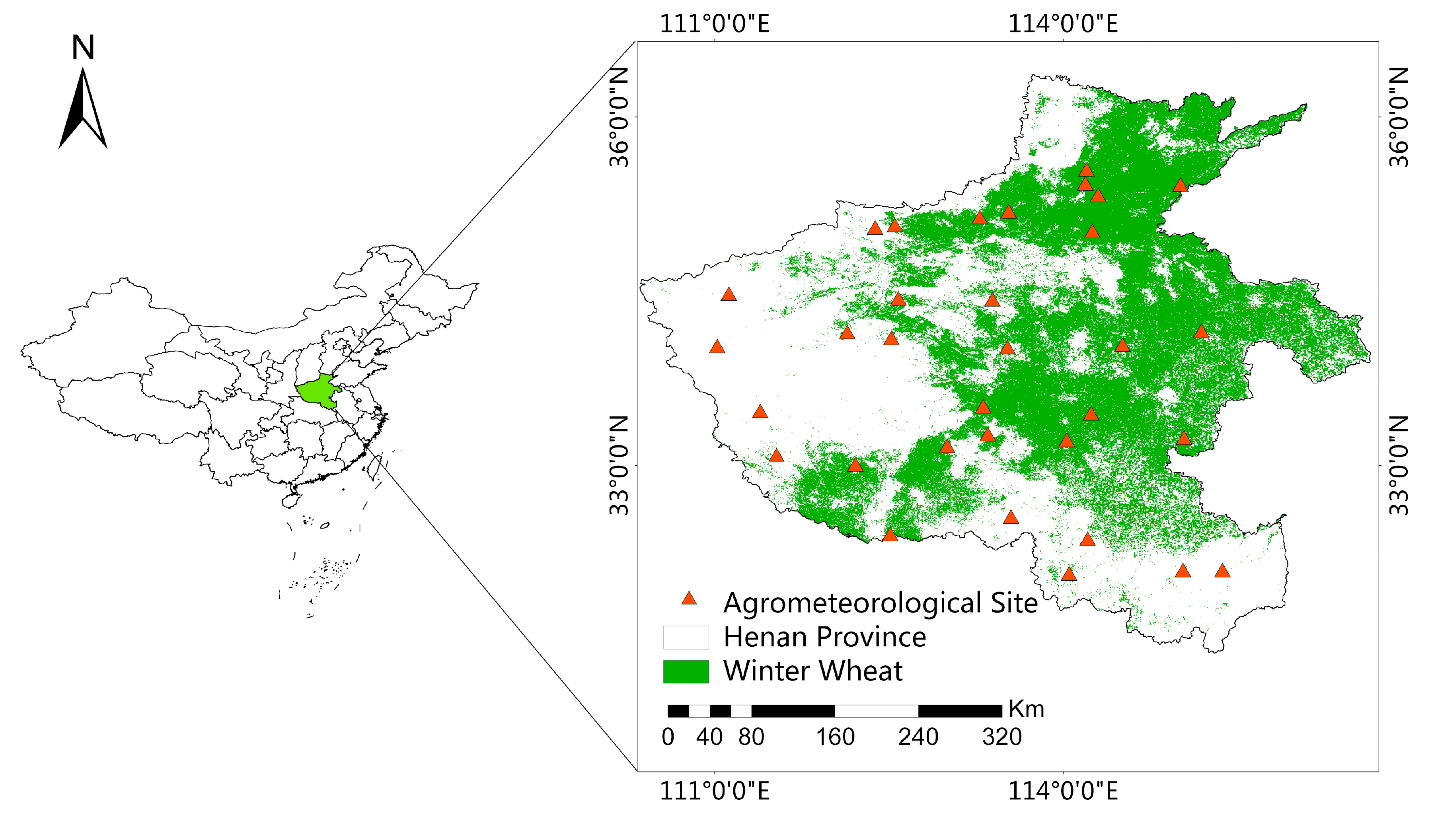
2.1. Study Area

This study was conducted in major winter wheat planting areas of Henan province of China, which extended from 31.38° N to 36.37° N and 110.35° E to 116.64° E. The winter wheat planting region in this province was selected as the study area, which was about 5.425 × 10⁶ ha and covered approximately one quarter of the entire winter wheat planting area of China (Data Source: National Bureau of Statistics of China, http://www.stats.gov.cn/). This region located in North China Plain as well as the warm temperate monsoon climate region, characterized by average annual precipitation of about 407.7–1295.8 mm, the average annual temperature of about 10.5–16.7 ℃ from south to north and annual average sunshine duration of about 1285.7–2292.9 h, which is favorable for winter wheat cultivation (Data Source: National Bureau of Statistics of China, http://www.gov.cn/guoqing/2018-01/17/content_5257444.htm). In this study, 30-m winter wheat planting map is extracted from Landsat8 OLI and Sentinel 2 data by means of random forest method [23,24]. Winter wheat in the study area usually sows from October to November and harvest during May and June in the following year. Due to different weather conditions and sowing dates, the maturity dates show large spatial variations in the study area. Figure 1 shows locations of agrometeorological stations and field distribution of the study area.

2.2. Data Preparation

2.2.1. Moderate Resolution Imaging Spectroradiometer (MODIS) Data

MODIS leaf area index (LAI) product (MCD15A3H) with spatial and temporal resolution of 500 m and 4 days, respectively, covering most of the growing season of winter wheat in study area (DOY 305~DOY 365 of 2017, DOY 1~DOY 150 of 2018) from 2017 to 2018 was collected (https://ladsweb.modaps.eosdis.nasa.gov/). The LAI time series were generated by stacking the images in temporal order and then reconstructed by the upper-envelope-based Savitzky–Golay (S-G) filter [25,26] to suppress the noise caused by clouds, water vapor, and aerosols.

S-G filter was proposed by Abraham Savitzky and MarcelJ. E. Golay in 1964. It is a weighted average algorithm of moving window, which is obtained by least square fitting of a given high-order polynomial in a sliding window. S-G filter can be expressed by Equation (1)

$$LA{I}_i^{sg}=\frac{{\sum }_{i=-m}^{i=m}{C}_{i}LA{I}_i}{N}$$

(1)

where $LA{I}_i$ is initial LAI value, $LA{I}_i^{sg}$ is S-G filtered LAI value, $C_i$ is the weight of $LA{I}_i$, m is the window radius, N is the number of all data in the window, which equals to 2m + 1.

However, the traditional S-G filter algorithm always causes the filtered points to be obviously close to the maximum or minimum value of the initial curve. So, we reconstructed the MODIS LAI time series by upper-envelope-based S-G filter. The upper-envelope-based S-G filter saves the original and S-G filtered LAI time series and generates the upper envelope of LAI time series as Equation (2):

$$LA{I}_t^l=\{\begin{array}{c}LA{I}_t^{sg} when LA{I}_t^{sg}\ge LA{I}_t^o\\ LA{I}_t^o when LA{I}_t^{sg}<LA{I}_t^o\end{array}$$

(2)

where $LA{I}_t^o$ is initial LAI at time node t obtained from MODIS LAI images, $LA{I}_t^{sg}$ is S-G filtered MODIS LAI, $LA{I}_t^l$ is the upper envelope of the two time series.

The absolute difference of upper envelope and S-G filtered LAI time series is used as the determination for exiting iteration, and is calculated as Equation (3):

$$dif={\displaystyle \sum _{t=1}^{t=n}}\left|LA{I}_t^l - LA{I}_t^{sg}\right|$$

(3)

where dif is the difference described as above. Then, the S-G filtered LAI time series will be iterated as the initial LAI time series by Equations (2) and (3) until dif reaches the threshold. In this study, the threshold was set as 0.5, which is an empirical value. If the threshold is greater than 0.5, the upper-enveloped-based S-G filter (UE-SG) filter curve is not smooth enough; if the threshold is less than 0.5, it will cost more time to finish UE-SG filter process. Figure 2 shows the comparison of MODIS LAI time series curves before and after upper-envelope-based S-G filtering.

2.2.2. Agrometeorology Data

Winter wheat data (including emergence, anthesis and maturity date, yield, biomass data of leaves, stems and ears at different stages, LAI, field water capacity, soil moisture) are collected from 33 agrometeorological stations in the study area from 2014 to 2018, and are conducive in recalibrating the World Food Studies (WOFOST) model. Observations from 2014 to 2016 are used for calibrating WOFOST, other data are used for verifying the accuracy of maturity prediction.

Table 1. General growth stages of winter wheat in Henan province.

Month	Oct.			Nov.			Dec.			Jan.			Feb.			Mar.			Apr.			May.			Jun.
Ten Days	1	2	3	1	2	3	1	2	3	1	2	3	1	2	3	1	2	3	1	2	3	1	2	3	1	2
Growth stage	Sowing stage		Emergence stage			Tillering stage		Wintering stage						Green-up stage			Jointing stage			Heading Anthesis stage		Grain filling stage		Milking-Maturidy stage
Zhengzhou Station			Nov. 5			Nov. 15		Dec. 7 (Start wintering)						Feb. 19			Mar. 19			Apr. 12		May. 8		May. 31
Fanqu Station			Nov. 4			Nov. 14		Dec. 6 (Start wintering)						Feb. 16			Mar. 18			Apr. 12		May. 6		May. 25

Note: 1, 2, and 3 represent the 1st, 2nd, and 3rd 10-day periods in each month.

shows the general growth stages of winter wheat in Henan province. Moreover, the observation date of each growth stage in Zhengzhou and Fanqu stations is also listed.

2.2.3. Meteorology Data and Weather Forecast

Meteorological data were obtained from China Regional Surface Meteorological Elements Dataset produced by Institute of Tibetan Plateau Research Chinese Academy of Sciences (http://www.tpedatabase.cn/portal/MetaDataInfo.jsp?MetaDataId=249369). We preprocessed meteorological data (including irradiation, minimum temperature, maximum temperature, early morning vapor pressure, wind speed at 2 meters and precipitation, with spatial and temporal resolution of 0.1° and 1 day, respectively, in a time resolution of 1 day and spatial resolution of 0.1°) to WOFOST weather input format [27,28]. This meteorology dataset has been increasingly used in agricultural research [29,30,31].

Weather forecast data in this study came from THORPEX Interactive Grand Global Ensemble (TIGGE) daily ensemble forecast data released by European Centre for Medium-Range Weather Forecasts (ECMWF, https://apps.ecmwf.int/datasets/data/tigge/levtype=sfc/type=cf/), which contains 6 elements (irradiation, minimum temperature, maximum temperature, early morning vapor pressure, wind speed at 2 meters and precipitation) required by WOFOST with spatial resolution of 0.25° and provides meteorological forecast data for the next 15 days. The TIGGE data were resampled from 0.25° to 500 m using nearest neighbor assignment method to match the assimilation unit size (500 m) of this study.

Since the TIGGE dataset used in this study can only provide weather forecast data for the following 15 days, the meteorological observation data and TIGGE forecast data cannot cover the entire growth period of winter wheat in the study area, when the forecasting node is set in March or April. Therefore, we used the most similar annual meteorological data at the same location from 1979 to 2016 to follow the weather forecast data exceeding the time limit of TIGGE by the methods proposed in the previous research [31,32]. The specific methods are as follows:

The six meteorological elements required by WOFOST from 1979 to 2016 are collected in grid format. The TIGGE ensemble prediction data from the selected forecasting start time to the next 15 d is acquired. Then, the highest temperature data of this time period arranged in chronological order make up a vector. Calculating the vectorial angle formed by this vector and vector of the same period in every year from 1979 to 2016, the year with the smallest angle is determined as the year with the highest similarity, and weather data of the determined year is used for the period that TIGGE data cannot cover. We use the Equation (4) to calculate the angle of two vectors:

$$\theta =arccos\frac{a·b}{\left|a\right|\left|b\right|}$$

(4)

In Equation (4), $a=\left(a_1,a_2,\dots ,a_n\right)$, $b=\left(b_1,b_2,\dots ,b_n\right)$, thus the Equation (4) can be described as Equation (5):

$$\theta =arccos\frac{{\sum }_{i=1}^n{a}_i{b}_i}{\sqrt{{\sum }_{i=1}^n{a}_i^2}\sqrt{{\sum }_{i=1}^n{b}_i^2}}$$

(5)

2.3. Parameterization of WOFOST Model

The WOFOST model was developed by the Wageningen University and Research Center of Wageningen, which aims to simulate crop growing process and reaction towards moisture, temperature, sunshine and other factors during the crop growth period. It provides quantification of developmental stages, estimates of biomass and grain yield at a daily time step for different crop types [33,34]. As a state variable, LAI can reflect the intensity of crucial processes such as photosynthesis, and it presents remarkable variation at different development stages. Therefore, it is a suitable state variable to adjust phenological growth by coupling remote sensing data and WOFOST model and optimizing relative parameters. The WOFOST model could run in different modes, e.g., potential mode, water-limited mode and nutrient-limited mode. Due to the good irrigation in the study area, we set the model to potential mode for this study.

The preprocessing of the WOFOST model is meant to re-calibrate and localize it for the target study area. In this study, we recalibrate the model manually based on observation data from Zhengzhou and Fanqu Stations, and our previous research [32,35,36]. The EFAST (Extend Fourier Amplitude Sensitivity Test) [37] algorithm was used to conduct a global sensitivity analysis for the WOFOST model. As for some wide-ranging and sensitive parameters like TSUM1 (effective heat sum from emergence to anthesis), TSUM2 (effective heat sum from anthesis to maturity) and IDEM (emergence date), we used the recorded date of emergence, anthesis, maturity and corresponding temperature data at all agrometeorological stations for the period 2014~2016 to calculate or determine the values of these parameters in these years, and then used the average values in these years to assign these parameters. Besides, we used the distance inverse weight (IDW) method to calculate the values of other pixels in the study area. For other parameters, we assigned one value to each parameter throughout the study area. As for the relatively stable parameters on spatial region, we determined the parameters by field measurements calculation. For example, we used the ratio of measured leaf area to leaf dry weight at various stages to determine the values of SLATB (specific leaf area as a function of development stage); the measured total dry weight increase in the crop and the increase in different organs (such as leaves, stems and ears) were used for calculating the values of parameters like FOTB (fraction of above ground dry matter increase partitioned to storage organs as a function of development stage), FSTB (fraction of above ground dry matter increase partitioned to stems as a function of development stage) and FLTB (fraction of above ground dry matter increase partitioned to leaves as a function of development stage). Furthermore, other parameters are calibrated according to previous research [32,35,36] or set as default value of WOFOST model.

2.4. Data Assimilation

2.4.1. Optimization Parameters Selection

The WOFOST model can simulate crop development stages by considering both temperature and photoperiod, or considering temperature only. In this study, the effect of photoperiod was not considered. Therefore, according to the principle of the WOFOST model, there are three dominating parameters in simulating the development stages despite the impact of photoperiod, which are emergence date (IDEM), effective heat sum from emergence to anthesis (TSUM1) and effective heat sum from anthesis to maturity (TSUM2). These parameters have significant spatial and temporal variations among years; therefore, we selected them as parameters to be optimized. Calibration of these parameters is based on historical data. Upper and lower values for the parameters are shown in

Table 2. Initial, upper and lower values of parameters.

Parameter	Unit	Initial Value	Lower Value	Upper Value
TSUM1	°C·d−1	954~1580	Initial value − 15%	Initial value + 15%
TSUM2	°C·d−1	543~917	Initial value − 20%	Initial value + 20%
IDEM	DOY	286~333	Initial value − 10	Initial value + 10

Note: TSUM1 means effective heat sum from emergence to anthesis, TSUM2 means effective heat sum from anthesis to maturity, IDEM means emergence date.

.

2.4.2. Cost Function and Shuffled Complex Evolution-University of Arizona (SCE-UA) Algorithm

In this study, the parameters were optimized by means of shuffled complex evolution-university of Arizona (SCE-UA). It is a global optimization algorithm developed by Duan in 1993 [38], which introduces complex shape segmentation and blending ideas. It has outstanding performance in the search space efficiency, computational speed, and global search optimization ability. In addition, the SCE-UA algorithm’s insensitivity to initial values of optimized parameters [39] and its advantages in optimization of nonlinear problems is manifest, thus it can reduce the requirement for prior knowledge when applying SCE-UA in coupling remote sensing and crop growth models [40,41,42]. It is worth mentioning that the SCE-UA algorithm was implemented by embedding it into the WOFOST model (Fortran Version).

According to previous research, the SCE-UA algorithm is more susceptible to the error of observation data than sequential assimilating algorithms [43]. Due to the mixed pixels and the impact of cloud and rain in 500-m resolution images, the value of MODIS LAI is often much lower than that of WOFOST model simulated LAI [44]. Therefore, we normalized LAI to solve this problem. That is, LAI from both the MODIS and WOFOST simulation are mapped to the range of 0 ~ 1, then the range of the two sources of LAI data are made the same while retaining the MODIS LAI trend information. The cost function is constructed as follows:

$$\mathrm{J}={\displaystyle \sum _{\mathrm{t}=1}^{\mathrm{n}}}{\left(\frac{{\mathrm{LAI}}_{\mathrm{obs}}^{\mathrm{t}}-{\mathrm{LAI}}_{\mathrm{obs}}^{\min }}{{\mathrm{LAI}}_{\mathrm{obs}}^{\max }-{\mathrm{LAI}}_{\mathrm{obs}}^{\min }} - \frac{{\mathrm{LAI}}_{\mathrm{sim}}^{\mathrm{t}} - {\mathrm{LAI}}_{\mathrm{sim}}^{\min }}{{\mathrm{LAI}}_{\mathrm{sim}}^{\max } - {\mathrm{LAI}}_{\mathrm{sim}}^{\min }}\right)}^2$$

(6)

${\mathrm{LAI}}_{\mathrm{obs}}^{\mathrm{t}}$ and ${\mathrm{LAI}}_{\mathrm{sim}}^{\mathrm{t}}$ are MODIS LAI and simulated LAI on t-day. ${\mathrm{LAI}}_{\mathrm{obs}}^{\max }$ and ${\mathrm{LAI}}_{\mathrm{sim}}^{\max }$ are maximum of MODIS LAI and simulated LAI. ${\mathrm{LAI}}_{\mathrm{obs}}^{\min }$ and ${\mathrm{LAI}}_{\mathrm{sim}}^{\min }$ are minimum of MODIS LAI and simulated LAI. J is the value of cost function. During five consecutive iterations, if all of J’s reach the threshold, SCE-UA stops and returns the optimal parameters set. Otherwise, if loops of iterations exceed the selected, the output parameter set will also be used as the optimal set. Then, we put this set into WOFOST model and run the whole framework.

3. Results

3.1. Validation of Calibrated WOFOST Model

In this section, we collected field measured LAI from Zhengzhou and Fanqu stations from 2014 to 2016 to verify the calibration result. Figure 3 shows the LAI time series simulated by calibrated WOFOST and the LAI field measurement.

WOFOST-simulated LAI of winter wheat varies during the whole growth period: LAI increases slowly at the emergence stage, keeps constant before the overwintering stage, increases rapidly since the greening stage, reaches its maximum before the anthesis stage, gradually decreases from the anthesis stage to the maturity stage and decreases rapidly after the maturity. As can be seen in Figure 3, the trend and characteristics of simulated LAI time series at the two stations are basically consistent with the measured LAI. After calculating the difference between these two sources of LAI, the root mean square error (RMSE) of the two stations in the period 2014~2016 is 0.94 m²/m², which indicates that the calibrated WOFOST model could simulate the LAI of the whole growth period well.

In addition, it can be seen from Figure 3 that there are uncertainties in some stations. There are two possible reasons: first, the inter-annual uncertainty exists in winter wheat field management, such as changes of the sowing date. These changes could cause some errors if we use the same set of crop parameters to simulate the development stages of winter wheat of various years, thus affect the accuracy of LAI simulation. Second, because the model calibration is based on the historical observation data of Zhengzhou Station, it is not necessarily suitable for winter wheat in other regions or other varieties.

Comparing the simulated LAI time series of Zhengzhou and Fanqu Stations from 2014 to 2016, it can be seen that the growth rate of winter wheat planted in Fanqu station is higher than that of Zhengzhou Station before wintering. A possible explanation is that the sowing date of Fanqu is earlier than that of Zhengzhou, because by observing the 2014 LAI time series, we can see the length from emergence to wintering of winter wheat in Zhengzhou Station is significantly shorter than that in the Fanqu, while the lower threshold temperature for ageing of leaves (TBASE) values in the two stations are set the same, and the climatic conditions of the two stations are relatively similar. Besides, it can also be seen that winter wheat in Zhengzhou grows faster than that in Fanqu from the green-up stages. Therefore, the change in sowing date has a great impact on the growth of winter wheat.

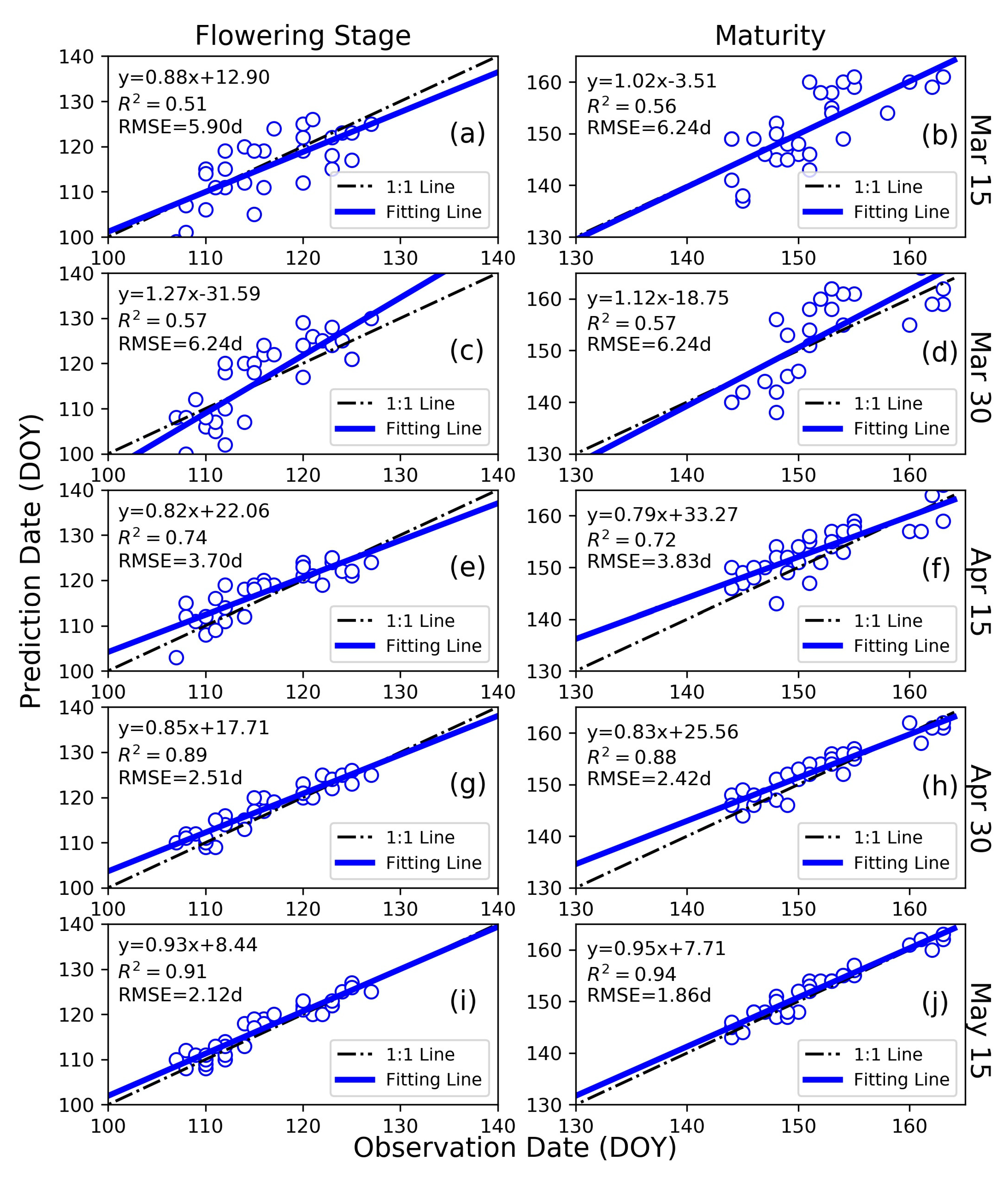
3.2. Accuracy of Maturity Prediction

3.2.1. Validation at Agrometeorological Stations Scale

In this section, we used LAI as the assimilating variable, MODIS LAI as the remote sensing data source, observed and forecast meteorological data as the weather input of WOFOST model, and 15 May 2018 as the forecasting start time. We constructed a normalized cost function (J) based on MODIS LAI and WOFOST-simulated LAI. The SCE-UA algorithm is used to minimize the J to optimize the parameters for WOFOST crop model. This optimized parameter set is used to drive the WOFOST model to simulate the winter wheat growth process of each pixel in the study area, and retrieve the maturity prediction.

The anthesis stage is an important demarcation period for the transition from vegetative growth to reproductive growth of a crop. It is a crucial indicator for the evaluation of the framework in phenological development simulation well. Therefore, in this study, we use the observed dates of the anthesis and maturity recorded by the agrometeorological stations in the study area to test the prediction results jointly. Figure 4 shows MODIS LAI, WOFOST-simulated LAI at Huaxian Station without and with data assimilation, respectively. Figure 5 is the scatter plot between the predicted and observed dates of the anthesis and maturity.

In Figure 4, the maturity date exhibited on the non-assimilated curve is DAE (days after emergence) 232, which is 10 days later than the observed date, while the assimilated maturity date is very close to the observed maturity date, which greatly improved the prediction accuracy of the maturity date. Besides, the variation trend of the assimilated LAI curve is closer to that of the MODIS LAI, which demonstrates that the optimization of parameters such as TSUM1 can actually optimize output LAI curve trend and avoid being affected by the difference between MODIS LAI and WOFOST simulated LAI. Figure 4 can provide an explanation for this: the non-assimilated anthesis date is DAE 177, which is also later than the observed date. After assimilation, we can see that the curve’s trend around the anthesis stage is much closer to the observed data and remotely sensed data, especially the anthesis period is pushed earlier. The assimilated anthesis date is DAE 173 and more in line with the observed date. From the results we can see that the assimilation framework significantly improves the prediction accuracy of the anthesis date, and further improves the prediction accuracy of the maturity date.

In addition, we can also find another effect brought by the accuracy improvement of maturity date, which is to adjust the range of the WOFOST simulated LAI. By analyzing the meteorological data of Zhengzhou Station and the daily activities simulation of winter wheat in the WOFOST model, we found if the simulated anthesis date is later than the observed date, it would lead to the winter wheat growing in a relatively warm environment in the greening and anthesis stage simulation, in which the temperature is higher, and the TSUM1 becomes bigger. It would result in the higher rate of growth and the higher peak of LAI output, which is bigger than six (Figure 4 green line); after assimilation, the simulated anthesis period is earlier, which is DAE 173 and this means the TSUM1 is lower than that without assimilation, thus reduced the LAI peak which is smaller than six (Figure 4 blue line). Therefore, the errors in the phenological growing stages will directly affect the range of LAI, and have a great impact on the simulation accuracy of the WOFOST model in terms of biomass and yield.

Figure 5c,d show that the anthesis date and maturity date after assimilation basically coincide with the observation, and the slope of the trend line of the scattered points is around one, indicating that the assimilated anthesis date and maturity date are consistent with the observed date, with RMSEs of 2.12 d and 1.86 d, respectively. Therefore, this framework can predict the maturity of winter wheat accurately.

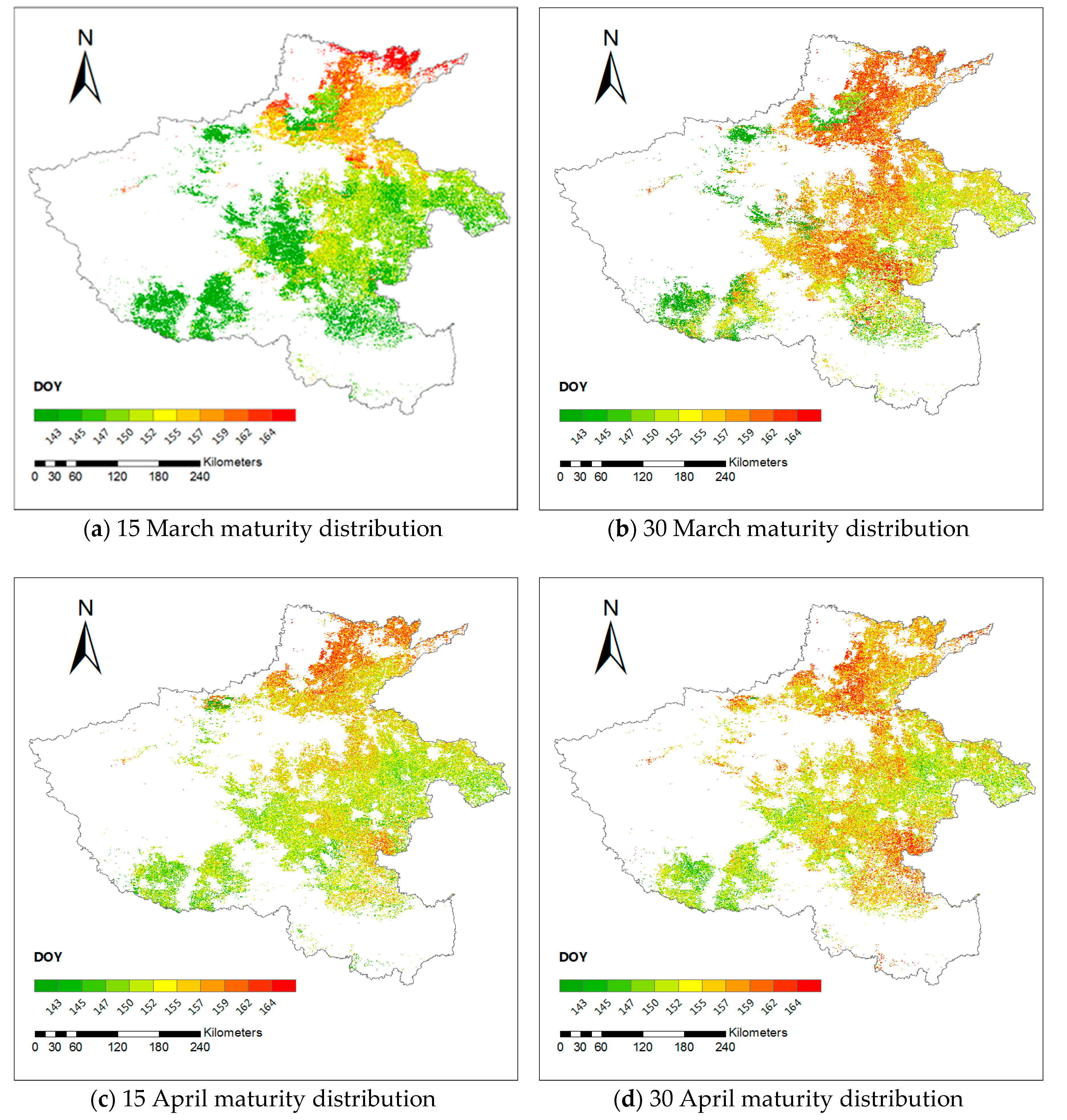
3.2.2. Spatial Distribution Comparison of WOFOST-Predicted Maturity Date without and with Data Assimilation

Figure 6 shows the spatial distribution comparison of WOFOST-predicted maturity date without and with data assimilation. The spatial difference in Figure 6a is not obvious, which illustrated that maturity dates were mostly influenced by meteorological data and the spatial distribution of IDEM, TSUM1 and TSUM2 after IDW method (Section 2.3) when crop model is not assimilated with remotely sensed LAI. Due to the coarse spatial resolution of the weather input data and the setting of the IDW calibration method, the predicted maturity dates without assimilation had obvious patch distribution, and the maturity date of one pixel is often very close to its neighbors. However, the spatial variability of the maturity dates become obvious after data assimilation with MODIS-LAI (Figure 6b) which demonstrated the fact that using MODIS-LAI data enables us to account for local conditions (e.g., soil, farming practices, and weather conditions) and reduce their uncertainty effects on the maturity date simulations. In the southern part of the study area, due to the earlier sowing time of winter wheat and suitable climate, the maturity date is the earliest, followed by the central and eastern regions. However, there are still some mismatches. For example, some places in the southeast region appear to harvest late, which is related to the local planting habits because planting later naturally results in a later harvest. The northeast region is a bit limited in terms of light and heat due to higher latitude and has the latest maturity date. The overall trend of maturity of wheat from both without and with data assimilation is gradually pushed back from the southwest to the northeast, however, after assimilation, the maturity dates of both the west and northeast regions are the latest.

The changes in the spatial distribution of the maturity date without and with data assimilation are mainly manifested in two aspects: (1) the assimilated maturity dates of the study area are generally postponed, especially in the high-altitude regions at the western part. The reasons for the analysis are the optimized IDEM and TSUM1. The optimized value has changed greatly from the initial calibrated value, leading to a remarkable trend change in the mature dates of the corresponding region after assimilation; (2) the maturity dates distribution after assimilation shows more detailed spatial variability. We can see that there are some certain differences in the maturity dates of adjacent winter wheat pixels. It demonstrates that the optimized parameters of WOFOST model by assimilating MODIS LAI can reflect the planting varieties and seeding time on a finer spatial scale to a certain extent.

3.3. Maturity Prediction with Different Forecasting Starting Time

3.3.1. Evaluation of Maturity Date Prediction Performance

In order to find out the prediction start time with higher accuracy as early as possible, we designed a set of predicting experiments. In this section, we selected five forecasting times to predict the maturity dates of winter wheat, which were 15 March, 30 March, 15 April, 30 April and 15 May (same as the experiment in Section 3.2).

Table 3. Time range of MODIS product and weather forecast data.

Forecasting Node	MODIS LAI	Meteorological Observation Data	TIGGE Data	Historical Meteorological Data
15 March	DOY 73	DOY 74	DOY 89	DOY 180
30 March	DOY 89	DOY 89	DOY 104	DOY 180
15 April	DOY 104	DOY 105	DOY 120	DOY 180
30 April	DOY 119	DOY 120	DOY 135	DOY 180
15 May	DOY 133	DOY 135	DOY 150	DOY 180

Note: TIGGE means THORPEX Interactive Grand Global Ensemble.

shows the time period of MODIS product (MCD15A3H) and meteorological data used in this study. Figure 7 exhibits the scatter plot of all the forecast starting times between observed and predicted dates.

Table 4. Accuracy of predicting anthesis and maturity date at different forecast starting times.

Forecasting Node	Anthesis Date		Maturity Date
	R2	RMSE (d)	R2	RMSE (d)
15 March	0.51	5.90	0.56	6.24
30 March	0.67	5.79	0.57	6.21
15 April	0.74	3.70	0.72	3.83
30 April	0.89	2.51	0.88	2.42
15 May	0.91	2.12	0.94	1.86

Note: RMSE means root mean square error.

shows the errors in those predictions.

It can be seen from the Figure 7 that both the two forecasting start times in March present large errors, the correlation between the predicted date and the observed dates is low, the correlation coefficient for the maturity dates is somewhat lower than that of the anthesis period, the scatter distribution is more dispersed, and the deviation of some points reaches 10 d. However, we found that the slope of the trend line between the predicted date and the observed date is about 1, which indicates that although there is a large error in the predicted growth period, there is no obvious systematic error (the intercept is between −3.51 and 33.27), and the overall deviation of the predicted value does not appear because the points are distributed around the 1:1 line in general.

Comparing the prediction results of 15 March with 30 March, it can be found that the errors of the two maturity periods are similar, but the prediction accuracy and consistency of the latter one in predicting anthesis date are improved. A feasible explanation is that most of the winter wheat in the study area enters the greening stage in mid-to-late February. After returning to green, the growth rate gradually increases. Therefore, winter wheat still grows slowly in the March 15 forecast experiment. Remote sensing LAI can only provide little trend variation, so the parameter optimization of the assimilation algorithm is not effective under this circumstance. On 30 March, as winter wheat enters the jointing stage, the trend of remote sensing LAI changes became more obvious, and the assimilation framework can improve the predicting accuracy of the anthesis stage to a certain extent.

The increase in RMSE is most obvious from 30 March to 15 April. The possible reason for the increase is that most of the winter wheat in the study area enters the heading stage in early and mid-April. The heading stage is the period when the LAI peaks during the whole growth period of the winter wheat, so heading stage is generally the period when the remote sensing and model-simulated LAI has the largest difference. Then, the parameter optimization by the assimilation method can adjust the peak of the output LAI of the model, so that the error of the predicted maturity can be reduced.

From the prediction results on 30 April and 15 May, we have found that the error in predicting the anthesis dates is even higher than that of the maturity dates, which points out an advantage of the assimilation framework in this study. That is, this framework is less affected by error transmission. Errors of state variables will gradually accumulate during the simulating process, resulting in simulation errors at maturity often larger than anthesis. But this framework assimilates all available LAI data for the whole growth period, that is, in this framework, the anthesis and maturity stages are optimized at the same time. Therefore, it is very likely that although there are errors in the anthesis period, these errors will be compensated in the maturity stage.

It can be seen from Figure 7 that with the postponement of the forecast time, the accuracy of the prediction (simulation) of the anthesis and maturity dates of winter wheat in the study area has gradually improved. The RMSE on 15 April is within 4 days: this increases to 2.5 on 30 April. On 15 May, the maturity prediction error is within 2 d, which shows high accuracy. In addition, the correlation between the predicted and the observed dates is also increasing, R² is increasing from about 0.7 to more than 0.9. The range of predicted and observed dates is closer to each other, and the difference in spatial variability is small. Therefore, the error and correlation coefficient on 30 April are remarkably close to 15 May, which is an ideal forecasting start time.

3.3.2. Prediction Results of Maturity Date for Different Forecasting Nodes

In Figure 6 and Figure 8, we have found the winter wheat in the study area matures from the southwest region to the northeast, basically resulting from meteorological conditions such as solar radiation and temperature. However, there are some regions disobeying the overall trend in the study area. For example, winter wheat of the southeastern area matures later mainly due to the local field management such as the sowing date.

Figure 8 shows that since 15 April, the spatial pattern of the predicted maturity dates begins to gradually conform to the actual situation, that is, the maturity dates gradually delay from the southwest to the northeast in the study area. It is obvious that the predicted maturity dates of most stations fluctuate greatly during the two forecasts in March, and the direction of fluctuation may be opposite. The fluctuation range has decreased since 15 April. After 30 April, the fluctuation gradually converges and stabilizes. This indicates that forecasting the maturity date on 30 April can generate better prediction results in the study areas.

4. Discussion

4.1. Assimilation of Remotely Sensed LAI into WOFOST Model

LAI is the most commonly used state variable that connects remotely sensed observations and crop models, because it is involved in many important processes of crop growth, such as light interception, CO₂ assimilation and vegetation transpiration. The remotely sensed LAI observation used in this study is MODIS LAI product (MCD15A3H) with 500-m spatial resolution. In reality, the field parcel size in China is always smaller than 500 m × 500 m, and the coarse pixels usually result in LAI values obtained from highly heterogeneous surfaces and leading to large scaling effects. Therefore, LAI observations at a finer spatial resolution can effectively reduce the spatial mismatch between the crop model and LAI observations, and it is an efficient way to improve the performance of data assimilation results [45]. Besides, the cost function used in this study is built by least square method, which takes both remote sensing observations and crop model simulations into account. However, this method does not consider the uncertainty of both of them. Therefore, a more thoughtful cost function that considers the uncertainty of observation and crop model could be investigated in the future work, for example, the four-dimensional variational data assimilation cost function (4DVar) [46,47], it can integrate remote sensing LAI (observations), crop model-simulated LAI (model simulations) and their uncertainties [48].

4.2. Maturity Date Prediction Using Crop Model Data Assimilation Scheme

Crop maturity is essential for evaluating crop productivity and crop management. The proposed maturity dates prediction method based on crop model data assimilation scheme successfully predicts winter wheat maturity date in 2018 of Henan province, and it has the best prediction accuracy since 30 April (RMSE = 2.42 d). This method shows significant applicability and has the potential to be applied to other winter wheat planting regions. Besides, it could be better if the approximate dates of growth stages and the general trend characteristics of LAI in the target study area are obtained prior to the prediction of maturity date, because the premise of this method is that the WOFOST model is localized well. If that basic information is scarce, it is difficult to determine the initial value of the parameters to be optimized (e.g., TSUM1, TSUM2, IDEM). In that case, the selected ranges of parameters for the optimization have to be enlarged in order to find the optimal values in those ranges. Meanwhile, this will increase the workload and greatly reduce the calculation efficiency.

Although this method has general applicability, there are also some limitations to the use of this approach. First, crop growth phenology in the WOFOST model is determined by temperature and photoperiod, but we only optimized temperature-related parameters (TSUM1 and TSUM2) in the present study. Therefore, the photoperiod-related parameters should be considered in the data assimilation scheme in future work. Second, there are some uncertainties in the meteorological data with regard to exceeding the prediction time limit of TIGGE. In this study, the meteorological data after the prediction time of TIGGE were followed by the similar year’s data, and there is a certain deviation from the actual meteorological data. In future study, we can try some medium- and long-term weather forecasting methods, such as regional climate model and weather generator [49], to couple with crop model for crop growth phenology prediction.

4.3. Uncertainty of Maturity Prediction

Some errors of the assimilated results were caused by the uncertainty in this framework. First, MODIS LAI product may be affected by cloud or rain, and the reconstructing process could introduce new bias to LAI time series. Moreover, the spatial resolution of remote sensing data is relatively low, thereby some buildings or other vegetation may be mixed in the planting pixels of winter wheat, resulting in limited purity of winter wheat pixels in the study area, affecting the quality of remote sensing LAI data, and consequently introducing errors to the maturity prediction. Second, some primary parameters of WOFOST, such as AMAXTB or FLTB, were not recalibrated by pixels, so the unsuitability could also bring uncertainties. Third, in the process of minimizing the cost function by SCE-UA algorithm, it may be difficult to accurately find the global optimal parameter set that is closest to the actual situation, so there may be some errors in the optimized parameter set.

From the agricultural perspective, the maturity of winter wheat is mainly determined by both the species and the field management. As for the species, because of the differences in winter wheat varieties and field management in the study area, the spatial values of these parameters ordered by WOFOST cannot be obtained. Therefore, the same values of other parameters will also cause certain errors when running WOFOST model. This study explains the phenological difference between TSUM1 and TSUM2 parameterization. However, other factors could also change the growing process, such as the vernalization before flowering, and the drought during the reproductive period [50,51]. As for the field management, the sowing date is determined by farmers, which could directly define the phenological stage start. Besides, the irrigation is also important for winter wheat in the study area because most of this region needs irrigating, but some of them may not well irrigated. If winter wheat suffers from drought in the reproductive period, it could lead to an earlier maturity. Finally, because the measured data from agrometeorological sites were used for verifying the prediction accuracy of the growth stages, these data can only reflect the development stages of the field observed by the sites, and the scale may be much smaller than the MODIS LAI data. The difference in scale between the two data sources will also cause prediction errors.

5. Conclusions

In this study, a crop model data assimilation framework was constructed for retrieving the predicted maturity dates at the regional scale. We selected LAI as the assimilating variable, MODIS LAI as the remote sensing data source, meteorological observation and weather numeric forecasting data as the weather input of WOFOST model, and 15 May 2018 as the starting time node of forecasting. The parameters of WOFOST crop model was optimized by SCE-UA to minimize the normalized cost function. The conclusions of this research are as follows: (1) the predicted anthesis dates and maturity dates after assimilation basically coincide with observation, with RMSE of 2.12 d and 1.86 d, respectively. Therefore, this framework can predict the maturity of winter wheat accurately. Besides, this framework can optimize the parameters of WOFOST such as TSUM1 and actually optimize the output LAI curve trend and avoid being affected by the difference of the two sources of LAI. (2) Considering both the earlier forecasting time and the higher accuracy, predicting maturity on 30 April can obtain ideal results. In this study, we have found that with the postponement of the forecasting start time, the accuracy of the prediction (simulation) of the anthesis and maturity dates was gradually improved. The RMSE on 15 April is within 4 days, and decreases to about 2.5 days on 30 April. On 15 May, the maturity prediction error is within 2 days, showing a high accuracy. In addition, the correlation between the predicted and the observed dates is also increasing, with R² is increasing from about 0.7 to more than 0.9.

References

1. FAO. The Future of Food and Agriculture–Trends and Challenges; Annual Report; FAO: Rome, Italy, 2017. [Google Scholar]
2. Ghose, B. Food security and food self-sufficiency in China: From past to 2050. Food Energy Secur. 2014, 3, 86–95. [Google Scholar] [CrossRef]
3. Hoque, M.M.; Hoffmann, V. Safety and Quality of Food (Rice and Wheat) Distributed through Public Food Distribution System (PFDS) in Bangladesh: Results from Laboratory Tests for Selected Contaminants; International Food Policy Research Institute: Washington, DC, USA, 2019; Volume 4. [Google Scholar]
4. Dong, Y.; Wang, Y.Z. Seed shattering: From models to crops. Front. Plant Sci. 2015, 6, 476. [Google Scholar] [CrossRef] [PubMed]
5. Lian, Z.; Zhao, S.; Kuang, S. Application of Phenological Observation Data to Forecast of Wheat Harvest Period. China Agric. Meteorol. 2006, 27, 226–228. (In Chinese) [Google Scholar]
6. Huang, J.; Gómez-Dans, J.; Huang, H.; Ma, H.; Wu, Q.; Lewis, P.; Liang, S.; Chen, Z.; Xue, J.; Wu, Y.; et al. Assimilation of remote sensing into crop growth models: Current status and perspectives. Agric. For. Meteorol. 2019, 276, 107609. [Google Scholar] [CrossRef]
7. Cheng, Z.; Meng, J.; Wang, Y. Improving spring maize yield estimation at field scale by assimilating time-series HJ-1 CCD data into the WOFOST model using a new method with fast algorithms. Remote Sens. 2016, 8, 303. [Google Scholar] [CrossRef] [Green Version]
8. Su, W.; Huang, J.X.; Liu, D.S.; Zhang, M.Z. Retrieving Corn Canopy Leaf Area Index from Multitemporal Landsat Imagery and Terrestrial LiDAR Data. Remote Sens. 2019, 11, 572. [Google Scholar] [CrossRef] [Green Version]
9. Dall’Olmo, G.; Karnieli, A. Monitoring phenological cycles of desert ecosystems using NDVI and LST data derived from NOAA-AVHRR imagery. Int. J. Remote Sens. 2002, 23, 4055–4071. [Google Scholar] [CrossRef]
10. Sakamoto, T.; Yokozawa, M.; Toritani, H. A crop phenology detection method using time-series MODIS data. Remote Sens. Environ. 2005, 96, 366–374. [Google Scholar] [CrossRef]
11. Villegas, D.; Royo, C. Biomass Accumulation and Main Stem Elongation of Durum Wheat Grown under Mediterranean Conditions. Ann. Bot. 2001, 88, 617–627. [Google Scholar] [CrossRef] [Green Version]
12. Schwartz, M.; Reed, B.; White, M. Assessing satellite-derived start-of-season measures in the conterminous USA. Int. J. Climatol. 2002, 22, 1793–1805. [Google Scholar] [CrossRef]
13. Sellers, P.; Randall, D.; Collatz, G. A Revised Land Surface Parameterization (SiB2) for Atmospheric GCMS. Part I: Model Formulation. J. Clim. 1996, 9, 676–705. [Google Scholar] [CrossRef]
14. Han-ya, I.; Ishii, K.; Noguchi, N. Acquisition and analysis of wheat growth information using satellite and aerial vehicle imageries. In Proceedings of the 3rd Asian Conference on Precision Agriculture, Beijing, China, 14–17 October 2009. [Google Scholar]
15. Matisoo, J. Predicting mature date of winter wheat with HJ-1A/1B data. Trans. Chin. Soc. Agric. Eng. 2011, 27, 225–230. [Google Scholar]
16. Saranwong, S.; Sornsrivichai, J.; Kawano, S. Prediction of ripe-stage eating quality of mango fruit from its harvest quality measured nondestructively by near infrared spectroscopy. Postharvest Biol. Technol. 2004, 31, 137–145. [Google Scholar] [CrossRef]
17. Peirs, A.; Schenk, A.; Nicolaï, B. Effect of natural variability among apples on the accuracy of VIS-NIR calibration models for optimal harvest date predictions. Postharvest Biol. Technol. 2005, 35, 1–13. [Google Scholar] [CrossRef]
18. Slaughter, D.C.; Crisosto, C.H. Nondestructive internal quality assessment of kiwifruit using near-infrared spectroscopy. Semin. Food Anal. 1998, 3, 131–140. [Google Scholar]
19. Verger, A.; Filella, I.; Baret, F.; Penuelas, J. Vegetation baseline phenology from kilometric global LAI satellite products. Remote Sens. Environ. 2016, 178, 1–14. [Google Scholar] [CrossRef] [Green Version]
20. Ma, G.; Huang, J.; Wu, W. Assimilation of MODIS-LAI into the WOFOST model for forecasting regional winter wheat yield. Math. Comput. Model. 2013, 58, 634–643. [Google Scholar] [CrossRef]
21. Apipattanavis, S.; Bert, F.; Podestá, G. Linking weather generators and crop models for assessment of climate forecast outcomes. Agric. For. Meteorol. 2010, 150, 166–174. [Google Scholar] [CrossRef]
22. Li, Z. Winter Wheat Yield and Quality Prediction Based on DSSAT Model Based on Remote Sensing Data and Weather Forecast Data. Ph.D. Thesis, Zhejiang University, Zhejiang, China, 2016. (In Chinese). [Google Scholar]
23. Yang, N.; Liu, D.; Feng, Q.; Xiong, Q.; Zhang, L.; Ren, T.; Zhao, Y.; Zhu, D.; Huang, J. Large-Scale Crop Mapping Based on Machine Learning and Parallel Computation with Grids. Remote Sens. 2019, 11, 1500. [Google Scholar] [CrossRef] [Green Version]
24. Wang, X.; Huang, J.; Feng, Q.; Yin, D. Winter Wheat Yield Prediction at County Level and Uncertainty Analysis in Main Wheat-producing Regions of China with Deep Learning Approaches. Remote Sens. 2020, 12, 1744. [Google Scholar] [CrossRef]
25. Chen, J.; Jönsson, P.; Tamura, M. A simple method for reconstructing a high-quality NDVI time-series data set based on the Savitzky–Golay filter. Remote Sens. Environ. 2004, 91, 332–344. [Google Scholar] [CrossRef]
26. Savitzky, A.; Golay, M. Smoothing and Differentiation of Data by Simplified Least Squares Procedures. Anal. Chem. 1964, 36, 1627–1639. [Google Scholar] [CrossRef]
27. Yang, K.; He, J.; Tang, W. On downward shortwave and longwave radiations over high altitude regions: Observation and modeling in the Tibetan Plateau. Agric. For. Meteorol. 2010, 150, 38–46. [Google Scholar] [CrossRef]
28. Lin, C.; Zhi, X.; Han, Y. Multi-model super-ensemble prediction of surface temperature based on TIGGE data. J. Appl. Meteorol. 2009, 20, 706–712. (In Chinese) [Google Scholar]
29. Chen, Y.; Yang, K.; He, J. Improving land surface temperature modeling for dry land of China. J. Geophys. Res. Atmos. 2011, 116. [Google Scholar] [CrossRef]
30. Li, S. Research on Theory and Application of Multi-center Aggregate Forecast Based on Tigge; Nanjing University: Nanjing, China, 2016. (In Chinese) [Google Scholar]
31. Ma, H.; Huang, J.; Huang, H. Regional yield forecast based on historical meteorological data and WOFOST model. Trans. Chin. Soc. Agric. Mach. 2018, 49, 257–266. (In Chinese) [Google Scholar]
32. Huang, J.; Ma, H.; Su, W.; Zhang, X.; Huang, Y.; Fan, J.; Wu, W. Jointly assimilating MODIS LAI and et products into the swap model for winter wheat yield estimation. IEEE J. Sel. Top. Appl. Earth Obs. Remote Sens. 2015, 8, 4060–4071. [Google Scholar] [CrossRef]
33. Van Diepen, C.A.; Wolf, J.; Van Keulen, H.; Rappoldt, C. WOFOST: A simulation model of crop production. Soil Use Manag. 2010, 5, 16–24. [Google Scholar] [CrossRef]
34. Keulen, H.; Wolf, J.; Fresco, L. Modelling of agricultural production: Weather, soils and crops. Agric. Ecosyst. Environ. 1986, 30, 142–143. [Google Scholar]
35. Ma, H.; Huang, J.; Zhu, D.; Liu, J.; Su, W.; Zhang, C.; Fan, J. Estimating regional winter wheat yield by assimilation of time series of HJ-1 CCD NDVI into WOFOST–ACRM model with Ensemble Kalman Filter. Math. Comput. Model. 2013, 58, 759–770. [Google Scholar] [CrossRef]
36. Huang, J.; Sedano, F.; Huang, Y.; Ma, H.; Li, X.; Liang, S.; Tian, L.; Zhang, X.; Fan, J.; Wu, W. Assimilating a synthetic Kalman filter leaf area index series into the WOFOST model to improve regional winter wheat yield estimation. Agric. For. Meteorol. 2016, 216, 188–202. [Google Scholar] [CrossRef]
37. Saltelli, A.; Tarantola, S.; Chan, K.P.S. A quantitative model-independent method for global sensitivity analysis of model output. Technometrics 1999, 41, 39–56. [Google Scholar] [CrossRef]
38. Duan, Q.; Gupta, V.; Sorooshian, S. Shuffled complex evolution approach for effective and efficient global minimization. J. Optim. Theory Appl. 1993, 76, 501–521. [Google Scholar] [CrossRef]
39. Duan, Q.; Sorooshian, S.; Gupta, V. Optimal Use of the SCE-UA Global Optimization Method for Calibrating Watershed Models. J. Hydrol. 1994, 158, 265–284. [Google Scholar] [CrossRef]
40. Song, X.; Shu, Q.; Wang, H. Application of SCE-UA, Genetic Algorithm and Simplex Optimization Algorithm. J. Wuhan Univ. 2009, 42, 6–9. (In Chinese) [Google Scholar]
41. Dai, C.; Liang, Z. Multidimensional joint distribution calculation method and its application in hydrology. J. Hydraul. Eng. 2006, 37, 0160–0165. (In Chinese) [Google Scholar]
42. Yue, S. Joint probability distribution of annual maximum storm peaks and amounts as represented by daily rainfalls. Hydrol. Sci. J. 2000, 45, 315–326. [Google Scholar] [CrossRef]
43. Huang, J.; Ma, H.; Sedano, F.; Lewis, P.; Liang, S.; Wu, Q.; Su, W.; Zhang, X.; Zhu, D. Evaluation of regional estimates of winter wheat yield by assimilating three remotely sensed reflectance datasets into the coupled WOFOST–PROSAIL model. Eur. J. Agron. 2019, 102, 1–13. [Google Scholar] [CrossRef]
44. Huang, J.; Jia, S.; Ma, H.; Hou, Y.; He, L. Dynamic simulation of winter wheat growth process in main producing areas of China based on WOFOST model. Trans. Chin. Soc. Agric. Eng. 2017, 33, 222–228. (In Chinese) [Google Scholar]
45. Zhuo, W.; Huang, J.; Li, L.; Zhang, X.; Ma, H.; Gao, X.; Huang, H.; Xu, B.; Xiao, X. Assimilating Soil Moisture Retrieved from Sentinel-1 and Sentinel-2 Data into WOFOST Model to Improve Winter Wheat Yield Estimation. Remote Sens. 2019, 11, 1618. [Google Scholar] [CrossRef] [Green Version]
46. Liang, S.; Qin, J. Data assimilation methods for land surface variable estimation. In Advances in Land Remote Sensing: System, Modeling, Inversion and Application; Liang, S., Ed.; Springer: New York, NY, USA, 2008; pp. 319–339. [Google Scholar]
47. Dente, L.; Satalino, G.; Mattia, F.; Rinaldi, M. Assimilation of leaf area index derived from ASAR and MERIS data into CERES-Wheat model to map wheat yield. Remote Sens. Environ. 2008, 112, 1395–1407. [Google Scholar] [CrossRef]
48. Huang, J.; Tian, L.; Liang, S.; Ma, H.; Becker-Reshef, I.; Huang, Y.; Su, W.; Zhang, X.; Zhu, D.; Wu, W. Improving winter wheat yield estimation by assimilation of the leaf area index from Landsat TM and MODIS data into the WOFOST model. Agric. For. Meteorol. 2015, 204, 106–121. [Google Scholar] [CrossRef] [Green Version]
49. Lv, Z.; Liu, X.; Cao, W.; Zhu, Y. Climate change impacts on regional winter wheat production in main wheat production regions of China. Agric. For. Meteorol. 2013, 171, 234–248. [Google Scholar] [CrossRef]
50. Huang, J.; Zhuo, W.; Li, Y.; Huang, R.; Sedano, F.; Su, W.; Dong, J.; Tian, L.; Huang, Y.; Zhu, D.; et al. Comparison of three remotely sensed drought indices for assessing the impact of drought on winter wheat yield. Int. J. Digit. Earth 2018, 3, 1–23. [Google Scholar] [CrossRef]
51. Huang, R.; Huang, J.; Zhang, C.; Ma, H.; Zhuo, W.; Chen, Y.; Zhu, D.; Wu, Q.; Mansaray, L.R. Soil temperature estimation at different depths, using remotely-sensed data. J. Integr. Agric. 2020, 19, 277–290. [Google Scholar] [CrossRef]
Figure 1. Study area.
Remotesensing 12 02896 g001
Figure 2. Comparison of Moderate Resolution Imaging Spectroradiometer (MODIS) leaf area index (LAI) time series curves before and after upper-envelope-based Savitzky–Golay (S-G) filtering (notes: UE-SG means upper-enveloped-based S-G filter).
Remotesensing 12 02896 g002
Figure 3. World Food Studies (WOFOST)-simulated LAI time series and measured LAI at stations. (a) Fanqu in 2014; (b) Zhengzhou in 2014; (c) Fanqu in 2015; (d) Zhengzhou in 2015; (e) Fanqu in 2016; (f) Zhengzhou in 2016.
Remotesensing 12 02896 g003
Figure 4. LAI time series from observation, MODIS, WOFOST simulation without and with data assimilation (Zhengzhou Station). (Note: LAIWOFOST means WOFOST-simulated LAI without data assimilation; LAIDA means WOFOST-simulated LAI after data assimilation; LAIMODIS means MODIS LAI product; LAIObserve means observed LAI).
Remotesensing 12 02896 g004
Figure 5. Scatter plot between the observed and predicted dates (a) without assimilation of anthesis stage, (b) without assimilation of maturity stage, (c) with assimilation of anthesis stage, and (d) with assimilation of maturity stage.
Remotesensing 12 02896 g005
Figure 6. Comparison between simulated spatial maturity date without and with data assimilation. (a) Maturity date without assimilation; (b) Maturity date with assimilation.
Remotesensing 12 02896 g006
Figure 7. Scatter plot between observed date and predicted date of forecasting start time on (a) 15th March for flowering stage, (b) 15th March for maturity stage, (c) 30th March for flowering stage, (d) 30th March for maturity stage, (e) 15th April for flowering stage, (f) 15th April for maturity stage, (g) 30th April for flowering stage, (h) 30th April for maturity stage, (i) 15th May for flowering stage, and (j) 15th May for maturity stage.
Remotesensing 12 02896 g007
Figure 8. Prediction results of maturity date for different forecasting nodes. ((a) 15th March, (b) 30th March, (c) 15th April, (d) 30th April).
Remotesensing 12 02896 g008